| Issue |
A&A
Volume 683, March 2024
|
|
|---|---|---|
| Article Number | A125 | |
| Number of page(s) | 6 | |
| Section | Catalogs and data | |
| DOI | https://doi.org/10.1051/0004-6361/202348263 | |
| Published online | 15 March 2024 | |
Analysis of the public HARPS/ESO spectroscopic archive
Ca II H&K time series for the HARPS radial velocity database★
1
Department of Earth and Planetary Science, Weizmann Institute of Science,
Rehovot,
Israel
e-mail: This email address is being protected from spambots. You need JavaScript enabled to view it.
2
Hamburger Sternwarte, Universität Hamburg,
Gojenbergsweg 112,
21029
Hamburg,
Germany
3
Department of Astronomy, Faculty of Physics, Sofia University “St. Kliment Ohridski”,
5 James Bourchier Blvd.,
1164
Sofia,
Bulgaria
4
Max-Planck-Institut für Astronomie,
Königstuhl 17,
69117
Heidelberg,
Germany
5
Department of Physics, Ariel University,
Ariel
40700,
Israel
6
Zentrum für Astronomie der Universtät Heidelberg,
Landessternwarte, Königstuhl 12,
69117
Heidelberg,
Germany
7
Astrophysics Geophysics And Space Science Research Center, Ariel University,
Ariel
40700,
Israel
Received:
13
October
2023
Accepted:
16
January
2024
Abstract
Context. Magnetic activity is currently the primary limiting factor in radial velocity (RV) exoplanet searches. Even inactive stars, such as the Sun, exhibit RV jitter of the order of a few m s−1 due to active regions on their surfaces. Time series of chromospheric activity indicators, such as the Ca II H&K lines, can be utilized to reduce the impact of such activity phenomena on exoplanet search programmes. In addition, the identification and correction of instrumental effects can improve the precision of RV exoplanet surveys.
Aims. We aim to update the HARPS -RVBANK RV database and include an additional 3.5 yr of time series and Ca II H&K lines (R′HK) chromospheric activity indicators. This additional data will aid in the analysis of the impact of stellar magnetic activity on the RV time series obtained with the HARPS instrument. Our updated database aims to provide a valuable resource for the exoplanet community in understanding and mitigating the effects of such stellar magnetic activity on RV measurements.
Methods. The new HARPS-RVBANK database includes all stellar spectra obtained with the HARPS instrument prior to January 2022. The RVs corrected for small but significant nightly zero-point variations were calculated using an established method. The R′HK estimates were determined from both individual spectra and co-added template spectra with the use of model atmospheres. As input for our derivation of R′HK, we derived stellar parameters from co-added, high signal-to-noise ratio templates for a total of 3230 stars using the stellar parameter code SPECIES.
Results. The new version of the HARPS RV database has a total of 252 615 RVs of 5239 stars. Of these, 195 387 have R′HK values, which corresponds to 77% of all publicly available HARPS spectra. Currently, this is the largest public database of high-precision (down to ~1 m s−1) RVs, and the largest compilation of R′HK measurements. We also derived lower limits for the RV jitter of F-, G-, and K-type stars as a function of R′HK.
Key words: techniques: radial velocities / stars: activity / stars: late-type / planetary systems
Full Tables 1 and 4 are available at the CDS via anonymous ftp to cdsarc.cds.unistra.fr (138.79.128.5) or via https://cdsarc.cds.unistra.fr/viz-bin/cat/J/A+A/683/A125
© The Authors 2024
 Open Access article, published by EDP Sciences, under the terms of the Creative Commons Attribution License (https://creativecommons.org/licenses/by/4.0), which permits unrestricted use, distribution, and reproduction in any medium, provided the original work is properly cited.
This article is published in open access under the Subscribe to Open model. This email address is being protected from spambots. You need JavaScript enabled to view it. to support open access publication.
1 Introduction
While the transit method has led to the detection of a greater number of exoplanets compared to the radial velocity (RV) method, the RV technique remains a valuable tool in the detection and characterization of exoplanetary companions. This is because it does not require continuous observations over multiple planetary periods, enabling the discovery of planets with orbital periods of the order of the time span over which spectra have been collected. This time span can be several decades for stars observed by multiple facilities. As such, the RV method enables the creation of a representative sample of planetary companions without the need for continuous coverage.
The yield of a search for substellar companions via the radial velocity (RV) method using high-resolution spectrographs such as the High Accuracy Radial velocity Planet Searcher (HARPS) (Mayor et al. 2003) is increased by optimizing the RV extraction method (e.g. Zechmeister et al. 2018) and by correcting the RVs for nightly instrumental effects (e.g. Courcol et al. 2015; Tal-Or et al. 2019). Based on the publicly available HARPS spectra, Trifonov et al. (2020) published the HARPS-RVBANK, a catalogue of >212 000 corrected RVs, which have since been used by the community to confirm or discover planet candidates (e.g. Palatnick et al. 2021; Sreenivas et al. 2022) and estimate planet occurrence rates (Bashi et al. 2020).
Aside from the detrimental influence of instrumental effects, stellar magnetic activity has long been known to be the primary cause of RV jitter for a long time (Saar et al. 1998). In combination with stellar rotation, the presence of active regions on the stellar surface can result in quasi-periodic RV signals mimicking those caused by a substellar companion (Queloz et al. 2001; Dumusque et al. 2011; Reiners et al. 2013). While this RV noise is louder in younger and more active stars (Tal-Or et al. 2018; Brems et al. 2019), it has a more complex dependence on the spectral type (Dumusque et al. 2011). Even slow rotators with low levels of magnetic activity, such as our Sun, exhibit RV jitter of a few m s−1 (Marchwinski et al. 2015; Haywood et al. 2016; Collier Cameron et al. 2019), thus exceeding the nominal precision of state-of-the-art planet-hunting facilities such as the Echelle Sectrograph for Rocky Exoplanets and Stable Spectroscopic Observations (ESPRESSO; Pepe et al. 2014), and upcoming facilities.
Though efforts have been made to mitigate the effect of magnetic activity with various methods (Collier Cameron et al. 2021; Binnenfeld et al. 2022), the most reliable way to exclude false positive detections to date is to measure the stellar rotation period and demonstrate it to be different from the planetary candidate signal. This can be achieved by analysing photo-spheric activity indicators (i.e. light curves, McQuillan et al. 2014), or chromospheric lines such as Hα or Ca II H&K (e.g. Amado et al. 2021). In this publication, we present an update to the HARPS-RVBANK, which incorporates newly available observational data, including 252615 RVs of 5239 stars and measurements of the relative emission in the Ca II H&K lines,  , for 77% of all spectra. In Sect. 2, we provide details of our re-processing scheme with the Spectrum radial velocity analyser (SERVAL) pipeline, the nightly zero point (NZP) correction process, and the derivation of stellar parameters and
  from the public spectra. In Sect. 3, we present our results and provide a discussion on our findings. Finally, in Sect. 4, we present a summary and our conclusions.
2 Updating the HARPS-RVBANK
We obtained all available HARPS stellar spectra from the ESO archive1 that were observed prior to January 2022. These spectra were processed in the same manner as described in Trifonov et al. (2020). In addition to the data reduction software (DRS) products provided by HARPS, we calculated SERVAL RVs and various activity indices using the methodology described in Zechmeister et al. (2018, 2020). We also determined the data-driven NZP corrections for both the DRS and SERVAL RVs. Figure 1 shows the zero-point variations of post-SERVAL RVs. The 774 good NZPs (out of 1395 nights with useful data) have a weighted rms scatter of 1.8 m s−1 and a median error of 1.1 m s−1. Despite the 2020–2021 COVID-related observing gaps, the instrument’s zero-point behaviour does not differ much from what was reported in Trifonov et al. (2020).
In the first release of the HARPS-RVBANK, we only included targets with at least three usable spectra, as this was the minimum required for constructing a spectral template and obtaining precise RVs with SERVAL. In this second release of the HARPS-RVBANK, we extended the inclusion criteria to include targets with a single usable spectrum, significantly increasing the number of targets. While we could not compute meaningful SERVAL RVs and activity indices for these targets, we provide the original HARPS-DRS estimates and used their spectra to estimate Ca II H&K values, which is the primary focus of this work. From 2003 to the present, we retrieved 309 425 unique spectra from the ESO archive. Of those spectra, 12 136 were excluded due to their classification as solar spectra, Solar System objects, quasars (QSOs), and various transients. Additionally, 36765 spectra were not included in the HARPS-RVBANK due to failing the quality control check, which includes criteria - for example - being taken with an I2 cell, having an extremely low or high signal-to-noise ratio (S/N), or exhibiting other issues that prevent the extraction of meaningful results. The new HARPS-RVBANK consists of 252 615 unique spectra of 5239 targets2 that have passed the semi-automated quality control process (see, Trifonov et al. 2020, for details).
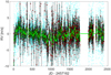 |
Fig. 1 Temporal evolution of NZPs. Black errorbars: HARPS-post SERVAL NZPs. Cyan dots: Stellar zero-point subtracted RVs of all RV-quiet stars (weighted RV rms scatter <10 m s−1). Red boxes: NZPs that were calculated with too few (<3) RVs. Red circles: NZPs with too large uncertainties (>1.2 m s−1). Magenta circles: significantly deviating NZPs. The RVs in the red-marked nights were corrected by using a smoothed version of the NZP curve, which was calculated with a moving weighted average (21-d window). For the ten significantly deviating NZPs, we adopted their individual (unsmoothed) NZP values, regardless of their uncertainties. Green dots: NZP values that were eventually used for the correction. |
2.1 Derivation of stellar parameters
The approach developed by Perdelwitz et al. (2021) requires precise stellar parameters, namely effective temperature (Teff), surface gravity (log g), metallicity ([Fe/H]), and rotational velocity (υ sin i). In order to ensure that the parameters are derived in as homogeneously a manner as possible, we used the publicly available code Spectroscopic Parameters and atmosphEric ChemIstriEs of Stars SPECIES3 (Soto & Jenkins 2018; Soto et al. 2021). The single-exposure HARPS spectra for each target were shifted to the rest frame and co-added. Only the resulting templates with an S/N≥ 20 were then processed with SPECIES, using the default line lists implemented in the code. Figure 2 shows the distribution of the S/N of all template spectra.
Since SPECIES is known to converge towards false effective temperatures for stars with Teff ≤ 4300 (Soto & Jenkins 2018; Soto et al. 2021), we adopted stellar parameters for all stars with color B − V > 1.24 from the latest version of the Transiting Exoplanet Survey Satellite (TESS) input catalogue (TIC v8.2 Stassun et al. 2019; Paegert et al. 2021). Out of a total of 5239 stars in the sample, we were able to derive stellar parameters for 3230 of them. The discrepancy is caused in most cases by a low S/N of the co-added spectrum, or stellar contamination by a close companion in others. Figures 3–5 show the comparison of the resulting effective temperature, surface gravity, and metallic-ity with those published in the latest version of the TESS input catalogue. While there is generally good agreement between the sets of parameters, we do advise that systematic errors in any derivation of stellar parameters may be larger than measured uncertainties (Torres et al. 2012).
The sample of targets for which all stellar parameters have been derived solely based on the HARPS spectra corresponds to a total of 172 948 single spectra, or 68.6% of the total. In order to increase this fraction, the remaining stars were cross-matched with the TESS input catalogue, which contains the effective temperature, surface gravity, and metallicity, but no rotational velocity. We, therefore, crossmatched the remaining sources with the Gaia DR3 catalogue (Gaia Collaboration 202la,b), yielding an additional 54 rotational velocity values. In the stellar parameter catalogue published along with this paper (see Table 1), which is available at the CDS, these targets are marked with uflag = 2 and those without any rotational velocity with υflag = 1.
Stellar parameters.
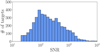 |
Fig. 2 Distribution of the S/N of the spectral templates used to compute stellar parameters. |
2.2 Extraction of R′HK
We followed the recipe of Perdelwitz et al. (2021), namely the computation of a grid of fluxes in six bands from PHOENIX models (Husser et al. 2013), with varying Teff, log g, and [Fe/H], where the grid step size follows that of the PHOENIX grid (see Table 1 in Husser et al. 2013). We adapted the edges of one bandpass (k1) with respect to those used in Perdelwitz et al. (2021) in order to minimize the number of absorption lines and hence the influence of errors caused by the determination of stellar metallicity. Table 2 lists the updated bandpasses, and Fig. 6 displays the bandpasses for three example model spectra. In addition to the parameters given by the PHOENIX grid, the spectra were artificially broadened with velocities in the range 1–200 km s−1 in order to account for stellar rotation. The measured spectra were then rectified in the regions of the Ca II H&K lines and normalized with regard to flux, the photospheric contribution in the lines was subtracted, and the resulting chromospheric excess was normalized with the bolometric flux, yielding  . As mentioned in Sect. 2.1, for some stars in the stellar parameter catalogue we were not able to determine υ sin i. During data reduction, υ sin i was set to 2 km s−1 for these targets. While the time series of these stars can be used to determine rotation periods or activity cycles,
  of these stars may be biased, which is why these entries are marked with the υflag in both the stellar parameter and the time series table. We determined
  for two sets of spectra:
- (i)
Individual measurements. To provide time series for individual targets, these values and their uncertainties are included as additional columns in the updated HARPS-RVBANK. Since the purpose of the single-measurement catalogue is the study of the time series of individual stars,
 was derived purely based on the uncertainty as to the flux.
 - (ii)
Co-added templates. To obtain an averaged, high-S/N value per target, the resulting
 are listed in the catalogue of stellar parameters described in Sect. 2.1. In order to allow for a comparison of the average activity levels of different stars, here, the uncertainties of the stellar parameters were included in the Monte Carlo approach for the error estimation.
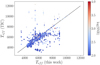 |
Fig. 3 Comparison of the effective temperature with literature values. The y-axis represents the values published in Stassun et al. (2019); Paegert et al. (2021), and the black dashed line represents equality. We note that the apparent tail of deviations towards lower temperatures is comprised of stars for which the RV was not known, and for which the stellar parameter determination failed. All stars with a missing RV value and possible errors in the catalogue are marked via the VFLAG column in our catalogue. |
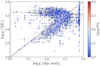 |
Fig. 4 Comparison of the surface gravity with literature values. The y-axis represents the values published by Stassun et al. (2019); Paegert et al. (2021), and the black dashed line represents equality. |
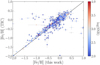 |
Fig. 5 Comparison of the metallicity with literature values. The y-axis represents the values published by Stassun et al. (2019); Paegert et al. (2021), and the black dashed line represents equality. |
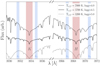 |
Fig. 6 Wavelength bands used for normalization and rectification of the spectra. The black lines show three examples of PHOENIX spectra with different stellar parameters. |
Updated wavelength bands used for rectification and flux extraction.
Overview of the number of spectra, and the source of the stellar parameters used for the derivation of  .
.
3 Results and discussion
Our analysis resulted in a total of 195 387  measurements, or ~77% of the entire HARPS-RVBANK. In the following, we give a short discussion of the relationship between
  and RV jitter, and compare our findings to previous results. Table 3 gives an overview of the statistics of the parameter derivation.
3.1 RV jitter as a function of activity and spectral type
The number of stars of spectral types F, G, and K in the sample is large enough to derive lower limits on the RV jitter as a function of the spectral type and activity level. Figure 7 shows the RV jitter σRV as a function of  derived from the co-added spectra for all main sequence stars of spectral types F, G, or K in the sample with at least 20 individual measurements. Here, we also excluded binaries with an RV jitter of σ-RV > 200 m s−1. For each spectral type, the sample was subdivided into activity levels with step sizes of 0.25 in log(
 ), and the 10th percentile of all RVs was adopted as the lower limit for each bin.
We derived the best-fit linear approximation for the lower limit of RV jitter of F-type stars to be
![Mathematical equation: $\log {\sigma _{{\rm{RV}}}}\left[ {{\rm{m}}{{\rm{s}}^{ - 1}}} \right] = 0.81 \times \log R_{{\rm{HK}}}^\prime + 4.55$](/articles/aa/full_html/2024/03/aa48263-23/aa48263-23-eq24.png) (1)
(1)
to be
![Mathematical equation: $\log {\sigma _{{\rm{RV}}}}\left[ {{\rm{m}}{{\rm{s}}^{ - 1}}} \right] = 0.91 \times \log R_{{\rm{HK}}}^\prime + 4.91$](/articles/aa/full_html/2024/03/aa48263-23/aa48263-23-eq25.png) (2)
(2)
for G-type ones, and
![Mathematical equation: $\log {\sigma _{{\rm{RV}}}}\left[ {{\rm{m}}{{\rm{s}}^{ - 1}}} \right] = 0.57 \times \log R_{{\rm{HK}}}^\prime + 3.04$](/articles/aa/full_html/2024/03/aa48263-23/aa48263-23-eq26.png) (3)
(3)
for K dwarfs.
3.2 Comparison to previous publications
Gomes da Silva et al. (2021) recently published a catalogue of chromospheric activity for a sample of 1674 FGK stars based on HARPS data. Since the underlying spectra are entirely included in our dataset, we compared the median  from their catalogue to that derived from our template spectra. Figure 8 shows that there are two types of systematic offset: (i) Cooler stars appear more active and (ii) most inactive stars exhibit lower
  in our catalogue, both relative to the values given by Gomes da Silva et al. (2021). While identifying the source of these systematics is beyond the scope of this paper, we tentatively conclude that it originates in the different methods for the extraction of
  . Our approach takes into account all stellar parameters including metallicity and rotational velocity, whereas the standard method of deriving
  , as carried out in Gomes da Silva et al. (2021), is the extraction of the Mount Wilson S index, which is subsequently converted to the excess chromo-spheric emission using a conversion based solely on the stellar colour (B − V).
Neglecting some stellar parameters in extracting  may be an oversimplification. For example, Schröder et al. (2009) found that fast stellar rotation leads to the Ca II H&K lines to be filled in, thus increasing the flux as determined by the classical Mount Wilson method. Furthermore, it has been found that
  is dependent on the stellar metallicity (Saar & Testa 2012). We conclude that any derivation of
  via a conversion factor that depends only on the stellar colour will likely be biased. Furthermore, as described in Perdelwitz et al. (2021), the method of using narrow bands close to the cores of the Ca II lines to rectify and normalize the spectra, while resulting in larger statistical errors compared to the classical approach, is less prone to systematics caused by irregularities in the order-merging or normalization of the pipeline-reduced spectra.
Updated HARPS-RVBANK.
 |
Fig. 7 RV jitter as a function of activity. The colour coding denotes the spectral type, and the dotted, solid, and dashed line correspond to the lower RV jitter for spectral types F, G, and K, respectively. |
4 Summary and conclusions
We present an update to the HARPS-RVBANK with newly calculated RVs, nightly zero points, and an addition of  for 77% of all spectra. Table 4 shows an example of five (out of 252 615) rows of the full catalogue. For 3230 stars, we were able to derive stellar parameters using co-added template spectra, which are available as a separate table. The updated RVs will enable the detection of new planet candidates in the same manner as the previous version of the HARPS-RVBANK (e.g. Feng et al. 2020; Sreenivas et al. 2022). The addition of the relative chro-mospheric emission in the Ca II H&K lines,
  , provides an additional tool for the study of stellar magnetic activity and the identification of false-positive planet detections caused by stellar rotation. The updated HARPS-RVBANK has already been used in several works on planet detection (Trifonov et al. 2022), stellar activity jitter (Kossakowski et al. 2022), and magnetic activity cycles (Fuhrmeister et al. 2023). While our
  values show colour-dependent systematic deviations compared to those derived in the classical way, that is, via the S index, we conclude that this is caused by the simplification made in the conversion with a factor that is solely a function of the stellar colour B – V.
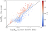 |
Fig. 8 Comparison of our median |

Acknowledgements
V.P. acknowledges funding through the Kimmel prize fellowship of the Center for Earth and Planetary Science at the Weizmann Institute of Science, and the Dean’s fellowship of the faculty of chemistry (WIS). T.T. acknowledges support by the BNSF programme ‘VIHREN-2021’ project No. KP-06-DV-5/15.12.2021. T.T. acknowledges support by the DFG Research Unit FOR 2544 ‘Blue Planets around Red Stars’ project No. KU 3625/2-1. This work was also funded by the Israel Science Foundation through grant No. 1404/22. Based on observations made with ESO Telescopes at the La Silla Paranal Observatory under programme IDs 0100.C-0097, 0100.C-0111, 0100.C-0414, 0100.C-0474, 0100.C-0487, 0100.C-0708, 0100.C-0746, 0100.C-0750, 0100.C-0808, 0100.C-0836, 0100.C-0847, 0100.C-0884, 0100.C-0888, 0100.D-0176, 0100.D-0273, 0100.D-0339, 0100.D-0444, 0100.D-0535, 0100.D-0776, 0101.C-0106, 0101.C-0232, 0101.C-0274, 0101.C-0275, 0101.C-0379, 0101.C-0407, 0101.C-0497, 0101.C-0510, 0101.C-0516, 0101.C-0623 , 0101.C-0788, 0101.C-0829, 0101.C-0889, 0101.D-0091, 0101.D-0465, 0101.D-0494, 0101.D-0697, 0102.A-0697, 0102.C-0171, 0102.C-0319, 0102.C-0338, 0102.C-0414, 0102.C-0451, 0102.C-0525, 0102.C-0558, 0102.C-0584, 0102.C-0618, 0102.C-0812, 0102.D-0119, 0102.D-0281, 0102.D-0483, 0102.D-0596, 0103.C-0206, 0103.C-0240, 0103.C-0432, 0103.C-0442, 0103.C-0472, 0103.C-0548, 0103.C-0719, 0103.C-0759, 0103.C-0785, 0103.C-0874, 0103.D-0445, 0104.C-0090, 0104.C-0358, 0104.C-0413, 0104.C-0418, 0104.C-0588, 0104.C-0849, 0104.C-0863, 072.A-0244, 072.C-0096, 072.C-0488, 072.C-0513, 072.C-0636, 072.D-0286, 072.D-0419, 072.D-0707, 073.A-0041, 073.C-0733 , 073.C-0784, 073.D-0038, 073.D-0136, 073.D-0527, 073.D-0578, 073.D-0590, 074.C-0012, 074.C-0037, 074.C-0061, 074.C-0102, 074.C-0221, 074.C-0364, 074.D-0131, 074.D-0380, 075.C-0087, 075.C-0140, 075.C-0202, 075.C-0234, 075.C-0332, 075.C-0689, 075.C-0710, 075.C-0756, 075.D-0194, 075.D-0600, 075.D-0614, 075.D-0760, 075.D-0800, 076.C-0010, 076.C-0073, 076.C-0155, 076.C-0279, 076.C-0429, 076.C-0878, 076.D-0103, 076.D-0130, 076.D-0158, 076.D-0207, 077.C-0012, 077.C-0080, 077.C-0101, 077.C-0295, 077.C-0364, 077.C-0513, 077.C-0530, 077.D-0085, 077.D-0498, 077.D-0633, 077.D-0720, 078.C-0037, 078.C-0044, 078.C-0133, 078.C-0209, 078.C-0233, 078.C-0403, 078.C-0510, 078.C-0751, 078.C-0833, 078.D-0067, 078.D-0071, 078.D-0245, 078.D-0299, 078.D-0492, 079.C-0046, 079.C-0127, 079.C-0170, 079.C-0329, 079.C-0463, 079.C-0657, 079.C-0681, 079.C-0828, 079.C-0898, 079.C-0927, 079.D-0009, 079.D-0075 , 079.D-0118, 079.D-0160, 079.D-0462, 079.D-0466, 080.C-0032, 080.C-0071, 080.C-0581, 080.C-0664, 080.C-0712, 080.D-0047, 080.D-0086, 080.D-0151, 080.D-0318, 080.D-0347, 080.D-0408, 081.C-0034, 081.C-0119, 081.C-0148, 081.C-0211, 081.C-0388, 081.C-0774, 081.C-0779, 081.C-0802, 081.C-0842, 081.D-0008, 081.D-0065, 081.D-0066, 081.D-0109, 081.D-0531, 081.D-0610, 081.D-0870, 082.B-0610, 082.C-0040, 082.C-0212, 082.C-0308, 082.C-0312, 082.C-0315, 082.C-0333, 082.C-0357, 082.C-0390, 082.C-0412, 082.C-0427, 082.C-0608, 082.C-0718, 082.D-0499, 082.D-0833, 083.C-0186, 083.C-0413, 083.C-0627, 083.C-0794, 083.C-1001, 083.D-0040, 083.D-0549, 083.D-0668, 083.D-1000, 084.C-0185, 084.C-0228, 084.C-0229, 084.C-1024, 084.C-1039, 084.D-0338, 084.D-0591, 085.C-0019, 085.C-0063, 085.C-0318, 085.C-0393, 085.C-0614, 085.D-0296, 085.D-0395, 086.C-0145, 086.C-0230, 086.C-0284, 086.C-0448, 086.D-0078, 086.D-0240, 086.D-0657, 087.C-0012, 087.C-0368, 087.C-0412, 087.C-0497, 087.C-0649, 087.C-0831, 087.C-0990, 087.D-0511, 087.D-0771, 087.D-0800, 088.C-0011, 088.C-0323, 088.C-0353, 088.C-0513, 088.C-0662, 088.D-0066, 089.C-0006, 089.C-0050, 089.C-0151, 089.C-0415, 089.C-0497, 089.C-0732, 089.C-0796, 089.D-0138, 089.D-0302, 089.D-0383, 090.C-0131, 090.C-0395, 090.C-0421, 090.C-0540, 090.C-0849, 090.D-0256, 091.C-0034, 091.C-0184, 091.C-0271, 091.C-0438, 091.C-0456, 091.C-0471, 091.C-0844, 091.C-0853, 091.C-0866, 091.C-0936, 091.D-0469, 091.D-0759, 091.D-0836, 092.C-0282, 092.C-0427, 092.C-0454, 092.C-0579, 092.C-0715, 092.C-0721, 092.C-0832, 092.D-0206, 092.D-0261, 092.D-0363, 093.C-0062, 093.C-0163, 093.C-0184, 093.C-0376, 093.C-0409, 093.C-0417, 093.C-0423, 093.C-0474, 093.C-0540, 093.C-0919, 093.D-0367, 093.D-0833, 094.C-0090, 094.C-0297, 094.C-0322, 094.C-0428, 094.C-0790, 094.C-0797, 094.C-0894, 094.C-0901, 094.C-0946, 094.D-0056, 094.D-0274, 094.D-0596, 094.D-0704, 095.C-0040, 095.C-0105, 095.C-0367, 095.C-0551, 095.C-0718, 095.C-0799, 095.C-0947, 095.D-0026, 095.D-0155, 095.D-0194, 095.D-0269, 095.D-0717, 096.C-0053, 096.C-0082, 096.C-0183, 096.C-0210, 096.C-0331, 096.C-0417, 096.C-0460, 096.C-0499, 096.C-0657, 096.C-0708, 096.C-0762, 096.C-0876, 096.D-0064, 096.D-0072, 096.D-0257, 096.D-0402, 097.C-0021, 097.C-0090, 097.C-0277, 097.C-0390, 097.C-0434, 097.C-0561, 097.C-0571, 097.C-0864, 097.C-0948, 097.C-1025, 097.D-0120, 097.D-0150, 097.D-0156, 097.D-0420, 098.C-0042, 098.C-0269, 098.C-0292, 098.C-0304, 098.C-0366, 098.C-0440, 098.C-0446, 098.C-0518, 098.C-0645, 098.C-0739, 098.C-0820, 098.C-0860, 098.D-0187, 099.C-0081, 099.C-0093, 099.C-0138, 099.C-0205, 099.C-0303, 099.C-0304, 099.C-0334, 099.C-0374, 099.C-0458, 099.C-0491, 099.C-0599, 099.C-0798, 099.C-0880, 099.C-0898, 099.D-0236, 099.D-0380, 105.2045.001, 105.2045.002, 105.207T.001, 105.208G.001, 105.20AK.002, 105.20AZ.001, 105.20B1.003, 105.20FX.001, 105.20G9.001, 105.20GX.001, 105.20L0.001, 105.20L8.002, 105.20MP.001, 105.20N0.001, 105.20NV.001, 105.20PH.001, 106.20Z1.001, 106.20Z1.002, 106.212H.001, 106.212H.007, 106.212H.009, 106.212H.010, 106.215E.001, 106.215E.002, 106.215E.004, 106.216H.001, 106.21DB.001, 106.21DH.001, 106.21ER.001, 106.21GB.003, 106.21MA.001, 106.21PJ.001, 106.21PJ.002, 106.21R4.001, 106.21TJ.001, 106.21TJ.008, 107.22R1.001, 107.22UN.001, 108.21XB.001, 108.21YY.001, 108.21YY.002, 108.21YY.004, 108.21YY.005, 108.222V.001, 108.2271.001, 108.2271.002, 108.2271.003, 108.229Z.001, 108.229Z.002, 108.22A8.001, 108.22CE.001, 108.22E7.001, 108.22KV.001, 108.22KV.002, 108.22KV.003, 108.22KV.004, 108.22KV.005, 108.22L8.001, 108.22LE.001, 108.22LR.001, 108.23MM.004, 108.23MM.005, 109.230J.001, 109.2317.001, 109.233Q.001, 109.2374.001, 109.2392.001, 109.239V.001, 109.23J8.001, 110.23XW.001, 110.23XW.002, 110.23YQ.001, 110.241K.001, 110.241K.002, 110.242T.001, 110.2434.001, 110.2438.001, 110.2460.001, 110.248C.001, 110.24BB.001, 110.24C8.001, 110.24C8.002, 110.24D8.001, 1101.C-0557, 1101.C-0721, 1102.C-0249, 1102.C-0339, 1102.C-0923, 1102.D-0954, 111.24PJ.002, 111.24UR.001, 111.24ZQ.001, 111.24ZW.001, 111.250B.001, 111.254A.001, 111.254E.001, 111.254R.002, 111.255C.001, 111.255C.003, 111.255C.004, 111.263V.001, 111.264X.001, 180.C-0886, 182.D-0356, 183.C-0437, 183.C-0972, 183.D-0729, 184.C-0639, 184.C-0815, 185.D-0056, 187.D-0917, 188.C-0265, 188.C-0779, 190.C-0027, 190.D-0237, 191.C-0505, 191.C-0873, 191.D-0255, 192.C-0224, 192.C-0852, 196.C-0042, 196.C-1006, 198.C-0169, 198.C-0836, 198.C-0838, 2101.C-5015, 276.C-5009, 281.D-5052, 281.D-5053, 281.D-5054, 282.C-5034, 282.C-5036, 282.D-5006, 283.C-5017, 283.C-5022, 288.C-5010, 289.C-5053, 289.D-5015, 292.C-5004, 295.C-5031, 295.C-5035, 297.C-5051, 495.L-0963, 60.A-9036, 60.A-9109, 60.A-9501, 60.A-9700, 60.A-9709. This work has made use of data from the European Space Agency (ES4A) mission Gaia (https://www.cosmos.esa.int/gaia), processed by the Gaia Data Processing and Analysis Consortium (DPAC, https://www.cosmos.esa.int/web/gaia/dpac/consortium). Funding for the DPAC has been provided by national institutions, in particular the institutions participating in the Gaia Multilateral Agreement.
References
- Amado, P. J., Bauer, F. F., Rodriguez López, C., et al. 2021, A&A, 650, A188 [NASA ADS] [CrossRef] [EDP Sciences] [Google Scholar]
- Bashi, D., Zucker, S., Adibekyan, V., et al. 2020, A&A, 643, A106 [NASA ADS] [CrossRef] [EDP Sciences] [Google Scholar]
- Binnenfeld, A., Shahaf, S., Anderson, R. I., & Zucker, S. 2022, A&A, 659, A189 [NASA ADS] [CrossRef] [EDP Sciences] [Google Scholar]
- Brems, S. S., Kürster, M., Trifonov, T., Reffert, S., & Quirrenbach, A. 2019, A&A, 632, A37 [EDP Sciences] [Google Scholar]
- Collier Cameron, A., Mortier, A., Phillips, D., et al. 2019, MNRAS, 487, 1082 [Google Scholar]
- Collier Cameron, A., Ford, E. B., Shahaf, S., et al. 2021, MNRAS, 505, 1699 [NASA ADS] [CrossRef] [Google Scholar]
- Courcol, B., Bouchy, F., Pepe, F., et al. 2015, A&A, 581, A38 [NASA ADS] [CrossRef] [EDP Sciences] [Google Scholar]
- Dumusque, X., Udry, S., Lovis, C., Santos, N. C., & Monteiro, M. J. P. F. G. 2011, A&A, 525, A140 [NASA ADS] [CrossRef] [EDP Sciences] [Google Scholar]
- Feng, F., Shectman, S. A., Clement, M. S., et al. 2020, ApJS, 250, 29 [Google Scholar]
- Fuhrmeister, B., Czesla, S., Perdelwitz, V., et al. 2023, A&A, 670, A71 [NASA ADS] [CrossRef] [EDP Sciences] [Google Scholar]
- Gaia Collaboration (Brown, A. G. A., et al.) 2021a, A&A, 649, A1 [NASA ADS] [CrossRef] [EDP Sciences] [Google Scholar]
- Gaia Collaboration (Luri, X., et al.) 2021b, A&A, 649, A7 [EDP Sciences] [Google Scholar]
- Gomes da Silva, J., Santos, N. C., Adibekyan, V., et al. 2021, A&A, 646, A77 [NASA ADS] [CrossRef] [EDP Sciences] [Google Scholar]
- Haywood, R. D., Collier Cameron, A., Unruh, Y. C., et al. 2016, MNRAS, 457, 3637 [Google Scholar]
- Husser, T. O., Wende-von Berg, S., Dreizler, S., et al. 2013, A&A, 553, A6 [NASA ADS] [CrossRef] [EDP Sciences] [Google Scholar]
- Kossakowski, D., Kürster, M., Henning, T., et al. 2022, A&A, 666, A143 [NASA ADS] [CrossRef] [EDP Sciences] [Google Scholar]
- Marchwinski, R. C., Mahadevan, S., Robertson, P., Ramsey, L., & Harder, J. 2015, ApJ, 798, 63 [Google Scholar]
- Mayor, M., Pepe, F., Queloz, D., et al. 2003, The Messenger, 114, 20 [NASA ADS] [Google Scholar]
- McQuillan, A., Mazeh, T., & Aigrain, S. 2014, ApJS, 211, 24 [Google Scholar]
- Paegert, M., Stassun, K. G., Collins, K. A., et al. 2021, arXiv e-prints [arXiv: 2108.04778] [Google Scholar]
- Palatnick, S., Kipping, D., & Yahalomi, D. 2021, ApJ, 909, L6 [NASA ADS] [CrossRef] [Google Scholar]
- Pepe, F., Molaro, P., Cristiani, S., et al. 2014, Astron. Nachr., 335, 8 [Google Scholar]
- Perdelwitz, V., Mittag, M., Tal-Or, L., et al. 2021, A&A, 652, A116 [NASA ADS] [CrossRef] [EDP Sciences] [Google Scholar]
- Queloz, D., Henry, G. W., Sivan, J. P., et al. 2001, A&A, 379, 279 [NASA ADS] [CrossRef] [EDP Sciences] [Google Scholar]
- Reiners, A., Shulyak, D., Anglada-Escudé, G., et al. 2013, A&A, 552, A103 [NASA ADS] [CrossRef] [EDP Sciences] [Google Scholar]
- Saar, S. H., & Testa, P. 2012, IAU Symp., 286, 335 [Google Scholar]
- Saar, S. H., Butler, R. P., & Marcy, G. W. 1998, ApJ, 498, L153 [NASA ADS] [CrossRef] [Google Scholar]
- Schröder, C., Reiners, A., & Schmitt, J. H. M. M. 2009, A&A, 493, 1099 [NASA ADS] [CrossRef] [EDP Sciences] [Google Scholar]
- Soto, M. G., & Jenkins, J. S. 2018, A&A, 615, A76 [NASA ADS] [CrossRef] [EDP Sciences] [Google Scholar]
- Soto, M. G., Jones, M. I., & Jenkins, J. S. 2021, A&A, 647, A157 [NASA ADS] [CrossRef] [EDP Sciences] [Google Scholar]
- Sreenivas, K. R., Perdelwitz, V., Tal-Or, L., et al. 2022, A&A, 660, A124 [NASA ADS] [CrossRef] [EDP Sciences] [Google Scholar]
- Stassun, K. G., Oelkers, R. J., Paegert, M., et al. 2019, AJ, 158, 138 [Google Scholar]
- Tal-Or, L., Zechmeister, M., Reiners, A., et al. 2018, A&A, 614, A122 [NASA ADS] [CrossRef] [EDP Sciences] [Google Scholar]
- Tal-Or, L., Trifonov, T., Zucker, S., Mazeh, T., & Zechmeister, M. 2019, MNRAS, 484, L8 [Google Scholar]
- Torres, G., Fischer, D. A., Sozzetti, A., et al. 2012, ApJ, 757, 161 [Google Scholar]
- Trifonov, T. 2019, Astrophysics Source Code Library [record ascl:1906.004] [Google Scholar]
- Trifonov, T., Tal-Or, L., Zechmeister, M., et al. 2020, A&A, 636, A74 [NASA ADS] [CrossRef] [EDP Sciences] [Google Scholar]
- Trifonov, T., Wollbold, A., Kürster, M., et al. 2022, AJ, 164, 156 [NASA ADS] [CrossRef] [Google Scholar]
- Zechmeister, M., Reiners, A., Amado, P. J., et al. 2018, A&A, 609, A12 [NASA ADS] [CrossRef] [EDP Sciences] [Google Scholar]
- Zechmeister, M., Reiners, A., Amado, P. J., et al. 2020, Astrophysics Source Code Library [record ascl:2006.011] [Google Scholar]
Instant access to the HARPS-RVBANK products is made available through the EXO-STRIKER exoplanet toolbox (Trifonov 2019), which can be freely accessed at https://github.com/3fon3fonov/exostriker
All Tables
Overview of the number of spectra, and the source of the stellar parameters used for the derivation of .
All Figures
|
Fig. 1 Temporal evolution of NZPs. Black errorbars: HARPS-post SERVAL NZPs. Cyan dots: Stellar zero-point subtracted RVs of all RV-quiet stars (weighted RV rms scatter <10 m s−1). Red boxes: NZPs that were calculated with too few (<3) RVs. Red circles: NZPs with too large uncertainties (>1.2 m s−1). Magenta circles: significantly deviating NZPs. The RVs in the red-marked nights were corrected by using a smoothed version of the NZP curve, which was calculated with a moving weighted average (21-d window). For the ten significantly deviating NZPs, we adopted their individual (unsmoothed) NZP values, regardless of their uncertainties. Green dots: NZP values that were eventually used for the correction. |
| In the text | |
|
Fig. 2 Distribution of the S/N of the spectral templates used to compute stellar parameters. |
| In the text | |
|
Fig. 3 Comparison of the effective temperature with literature values. The y-axis represents the values published in Stassun et al. (2019); Paegert et al. (2021), and the black dashed line represents equality. We note that the apparent tail of deviations towards lower temperatures is comprised of stars for which the RV was not known, and for which the stellar parameter determination failed. All stars with a missing RV value and possible errors in the catalogue are marked via the VFLAG column in our catalogue. |
| In the text | |
|
Fig. 4 Comparison of the surface gravity with literature values. The y-axis represents the values published by Stassun et al. (2019); Paegert et al. (2021), and the black dashed line represents equality. |
| In the text | |
|
Fig. 5 Comparison of the metallicity with literature values. The y-axis represents the values published by Stassun et al. (2019); Paegert et al. (2021), and the black dashed line represents equality. |
| In the text | |
|
Fig. 6 Wavelength bands used for normalization and rectification of the spectra. The black lines show three examples of PHOENIX spectra with different stellar parameters. |
| In the text | |
|
Fig. 7 RV jitter as a function of activity. The colour coding denotes the spectral type, and the dotted, solid, and dashed line correspond to the lower RV jitter for spectral types F, G, and K, respectively. |
| In the text | |
|
Fig. 8 Comparison of our median |
| In the text | |
Current usage metrics show cumulative count of Article Views (full-text article views including HTML views, PDF and ePub downloads, according to the available data) and Abstracts Views on Vision4Press platform.
Data correspond to usage on the plateform after 2015. The current usage metrics is available 48-96 hours after online publication and is updated daily on week days.
Initial download of the metrics may take a while.