| Issue |
A&A
Volume 683, March 2024
|
|
|---|---|---|
| Article Number | A133 | |
| Number of page(s) | 14 | |
| Section | Numerical methods and codes | |
| DOI | https://doi.org/10.1051/0004-6361/202348007 | |
| Published online | 15 March 2024 | |
TIPSY: Trajectory of Infalling Particles in Streamers around Young stars
Dynamical analysis of the streamers around S CrA and HL Tau★
1
European Southern Observatory,
Karl-Schwarzschild-Str. 2,
85748
Garching bei München,
Germany
e-mail: This email address is being protected from spambots. You need JavaScript enabled to view it.
2
Institute for Astronomy, University of Hawaii,
Honolulu,
HI
96822,
USA
3
University Observatory, Faculty of Physics, Ludwig-Maximilians-Universität München,
Scheinerstr. 1,
81679
Munich,
Germany
4
Exzellenzcluster ORIGINS,
Boltzmannstr. 2,
85748
Garching,
Germany
5
Niels Bohr Institute, University of Copenhagen,
Øster Voldgade 5,
1350
Copenhagen,
Denmark
6
Department of Astronomy, University of Virginia,
Charlottesville,
VA
22904,
USA
7
Max-Planck Institute for Extraterrestrial Physics,
Gießenbachstraße 1,
85748
Garching bei München,
Germany
8
Academia Sinica Institute of Astronomy and Astrophysics,
1, Sec. 4, Roosevelt Rd,
Taipei
10617,
Taiwan
Received:
18
September
2023
Accepted:
6
January
2024
Abstract
Context. Elongated trails of infalling gas, often referred to as “streamers,” have recently been observed around young stellar objects (YSOs) at different evolutionary stages. This asymmetric infall of material can significantly alter star and planet formation processes, especially in the more evolved YSOs.
Aims. In order to ascertain the infalling nature of observed streamer-like structures and then systematically characterize their dynamics, we developed the code TIPSY (Trajectory of Infalling Particles in Streamers around Young stars).
Methods. Using TIPSY, the streamer molecular line emission is first isolated from the disk emission. Then the streamer emission, which is effectively a point cloud in three-dimensional (3D) position–position–velocity space, is simplified to a curve-like representation. The observed streamer curve is then compared to the theoretical trajectories of infalling material. The best-fit trajectories are used to constrain streamer features, such as the specific energy, the specific angular momenta, the infall timescale, and the 3D morphology.
Results. We used TIPSY to fit molecular-line ALMA observations of streamers around a Class II binary system, S CrA, and a Class I/II protostar, HL Tau. Our results indicate that both of the streamers are consistent with infalling motion. For the S CrA streamer, we could constrain the dynamical parameters well and find it to be on a bound elliptical trajectory. On the other hand, the fitting uncertainties are substantially higher for the HL Tau streamer, likely due to the smaller spatial scales of the observations. TIPSY results and mass estimates suggest that S CrA and HL Tau are accreting material at a rate of ≳27 Mjupiter Myr–1 and ≳5 Mjupiter Myr–1, respectively, which can significantly increase the mass budget available to form planets.
Conclusions. TIPSY can be used to assess whether the morphology and kinematics of observed streamers are consistent with infalling motion and to characterize their dynamics, which is crucial for quantifying their impact on the protostellar systems.
Key words: methods: data analysis / planets and satellites: formation / protoplanetary disks / stars: formation / ISM: kinematics and dynamics
3D plots associated to Figs. 2 and 3 are available at https://www.aanda.org
© The Authors 2024
 Open Access article, published by EDP Sciences, under the terms of the Creative Commons Attribution License (https://creativecommons.org/licenses/by/4.0), which permits unrestricted use, distribution, and reproduction in any medium, provided the original work is properly cited.
This article is published in open access under the Subscribe to Open model. This email address is being protected from spambots. You need JavaScript enabled to view it. to support open access publication.
1 Introduction
The traditional picture of low-mass star formation assumes that protostars, together with their circumstellar disks, form due to the axisymmetric collapse of dense protostellar cores (e.g., Shu 1977; Terebey et al. 1984). Then, as the surrounding gas envelope disperses, protostars evolve from the embedded Class 0 and I stage to the Class II stage. These Class II systems are then traditionally assumed to evolve in isolation to form planetary systems, such as our Solar System.
However, stars form in turbulent giant molecular clouds, where the initial conditions for star and disk formation cannot be represented as isolated non-turbulent spheres (e.g. Pineda et al. 2023; Hacar et al. 2023). Numerical simulations of molecular clouds that follow the collapse of many protostellar cores show that the star-formation processes can be highly asymmetrical, with material usually falling onto protostellar systems via elongated channels, or “streamers” (e.g., Padoan et al. 2014; Haugbølle et al. 2018; Kuznetsova et al. 2019; Lebreuilly et al. 2021; Pelkonen et al. 2021; Kuffmeier et al. 2017, 2023). Recently, with the increased sensitivity of interferometric observations, such streamers have started to be observed around young stellar objects (YSOs) at various evolutionary stages, from the embedded Class 0 and I sources (e.g., Tobin et al. 2012; Yen et al. 2014; Tokuda et al. 2018; Pineda et al. 2020; Thieme et al. 2022; Valdivia-Mena et al. 2022; Murillo et al. 2022; Hsieh et al. 2023; Lee et al. 2023; Mercimek et al. 2023; Cacciapuoti et al. 2024) to the more evolved Class I/II and II sources (e.g., Tang et al. 2012; Akiyama et al. 2019; Yen et al. 2019; Alves et al. 2020; Garufi et al. 2022; Huang et al. 2020, 2021, 2022, 2023; Gupta et al. 2023). The Mailing streamers observed around more evolved YSOs further challenge our assumption that these systems evolve in isolation to form planetary systems; in reality, they are still embedded in large-scale molecular clouds (≳1 pc) and may continue to accrete material from them.
The infall of material in evolved sources can greatly influence the physical and chemical properties of protoplanetary disks and, thus, of the planets they form. For example, the supply of fresh material can help solve the “mass-budget problem” of protoplanetary disks, in which observations suggest that they are typically not massive enough to form the observed planetary systems (e.g., Manara et al. 2018; Mulders et al. 2021). Moreover, observations (Ginski et al. 2021) and simulations (Thies et al. 2011; Dullemond et al. 2019; Kuffmeier et al. 2021) have shown that material falling at these late stages can be dynamically different from the original parental core and can induce misalignments in disks. This can further explain the misalignments observed in evolved planetary systems (e.g., Albrecht et al. 2022). Late infall can also bring chemically different material to the system, which can explain the observed chemical diversity among meteorites (Nanne et al. 2019). Simulations (Vorobyov & Basu 2005; Dunham & Vorobyov 2012; Padoan et al. 2014; Jensen & Haugbølle 2018) have shown that infall-induced accretion bursts can naturally resolve the accretion luminosity problem in protostars (see Kenyon et al. 1990). Kuffmeier et al. (2023) demonstrated that infall of material onto Class II systems can also make them seem less evolved, which may affect studies on populations of YSOs. Finally, this phenomenon may also produce some of the observed protoplanetary disk substructures, such as rings (Kuznetsova et al. 2022), spirals (Hennebelle et al. 2017; Kuffmeier et al. 2018), and vortices (Bae et al. 2015).
However, the dynamics of observed streamers need to be characterized to assess their impact on the star and planet formation processes. This has only been done for a few streamers, using methods such as analyzing velocity gradients along the streamers in position–velocity space (e.g., Yen et al. 2014, 2019; Alves et al. 2020), qualitatively comparing infailing trajectories from Mendoza et al. (2009) to the streamer velocity gradients and morphologies (e.g., Pineda et al. 2020; Valdivia-Mena et al. 2022; Garufi et al. 2022), and fitting infalling trajectories determined using the Ulrich-Cassen-Moosman (UCM) model (e.g., Ulrich 1976; Cassen & Moosman 1981) to the streamer structures in position–position–velocity (PPV) space (Thieme et al. 2022). These studies suggest that infalling streamers can transfer significant mass to the protostellar systems. However, these parameters are usually estimated only for embedded sources, and the range of their possible values is generally not well constrained. For more evolved Class I/II and II sources, the infalling material can be dynamically unrelated to the protostellar system, and thus we need to explore a wider range of initial configurations to identify the infalling trajectories that best represent observed structures.
To address these issues, we have developed the code Trajectory of Infalling Particles in Streamers around Young Stars (TIPSY)1, which was designed to fit theoretical trajectories of infalling gas to molecular-line observations of streamers, without assuming any initial configuration (relative position and velocity) for the gas. We further used this code to analyze streamers around two evolved sources: the Class II binary system S CrA, for which a ~1000 au streamer-like structure was reported by Gupta et al. (2023), and the Class I/II system HL Tau, for which a kinematic analysis of a ~500 au streamer (Yen et al. 2019) and the corresponding shock observations (Garufi et al. 2022) suggest an infalling motion of gas. Evolved sources are also more suitable for this kind of analysis because the protostellar masses can be estimated independently of streamer modeling, as done by using spectroscopy for S CrA (Gahm et al. 2018) and via the modeling of a Keplerian disk for HL Tau (Yen et al. 2019).
The fitting methodology employed by TIPSY is detailed in Sect. 2. Subsequently, we demonstrate TIPSY by using it to analyze the streamers around S CrA (Sect. 3.1) and HL Tau (Sect. 3.2). The results are discussed in Sect. 4, and we conclude in Sect. 5.
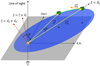 |
Fig. 1 Schematic diagram of coordinate axes used to compute the theoretical trajectories of infalling gas (green cloud) around a protostellar system (orange star), as discussed in Sect. 2.1. |


2 Fitting methodology
TIPSY fits theoretical trajectories expected for infalling gas, following the model given in Mendoza et al. (2009), to the molecular-line observations of streamers. The fitting is done in three-dimensional (3D) PPV space: right ascension (RA), declination (Dec), and line-of-sight (LOS) velocity or radial velocity (RV); in other words, the morphology and velocity gradient of streamers are fitted simultaneously. To define a general initial configuration of infalling gas, we needed to define the 3D position  and velocity
  vectors relative to the protostar (see Fig. 1). Relative position in RA and Dec direction as well as the relative speed in the LOS direction can be inferred directly from the observations. The remaining three parameters, required to define an initial configuration, are the separation in the LOS direction and the relative speeds in the RA and Dec directions. For a range of possible initial configurations, we computed theoretical trajectories (see Sect. 2.1) and compared them to the observations (see Sect. 2.2 and Figs. 2 and 3). The distribution of free parameters with reasonable fits was used to estimate uncertainties (see Sect. 2.3 and Fig. 4). Some of the known caveats associated with this kind of analysis are mentioned in Sect. 2.4.
The idea of comparing streamer observations to the Mailing trajectories in the PPV space is similar to the fitting of UCM trajectories to elongated structures around the Class 0 proto-star Lupus 3-MMS by Thieme et al. (2022). However, the UCM model assumes the particle to be in a parabolic orbit with no initial RV (e.g., Ulrich 1976). Moreover, Thieme et al. (2022) had to make further assumptions about the configuration of infalling gas, for example an initial radius of 10000 au and a final centrifugal radius of 105 au. Such assumptions are less likely to be valid for more evolved (Class I/II and II) sources because the infalling material can be dynamically unrelated to the original parental core of the protostellar system.
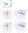 |
Fig. 2 Flow of S CrA 13CO (2–1) data in the TIPSY pipeline. Panel a: intensity-weighted velocity (moment 1) map in colors, overlaid with contours representing the integrated intensity (moment 0; see Fig. E.1). The red segments in the bottom-left corners depict a length scale of 1000 au. The pink ellipses in the bottom-right corners depicts the beam size of the data. Panel b: isometric projection of the 3D PPV diagram of pixels with intensity >5σ in the whole field of view. Panel c: isometric projection of the PPV diagram of an isolated and cleaned streamer. The red square and its error bars represent intensity-weighted means and standard deviations, respectively. Panel d: same as panel c, but with the best-fit trajectory, as represented by the black line. Black circles denote the interpolated values of the theoretical trajectory, which are directly compared to the intensity-weighted means. Panel e: same as panel b, but with the best-fit trajectory, as represented by the black line. 3D interactive versions of panels d and e are available online. |
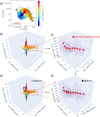 |
Fig. 3 Same procedure as described in Fig. 2, but for HL Tau instead of S CrA. 3D interactive versions of panels d and e are available online. |
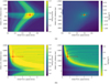 |
Fig. 4 Distribution of goodness-of-fit estimates as functions of free parameters: initial speed on the POS (x-axis) and initial spatial offset in the LOS direction, for TIPSY fitting for S CrA (top panels) and HL Tau (bottom panels). Here, initial direction of gas in the POS (third free parameter) is fixed to the value for the best fit. Left panels: distribution of fractions of coordinate values of points in the observed streamer curve (intensity-weighted means and standard deviations), which is consistent with the theoretical trajectories. Right panels: distribution of log(log(χ2)) deviations between the observed streamer curve and theoretical trajectories. In all the plots, yellow regions represent good fits. Red squares represent the best fit, as discussed in Sect. 2.2. The red lines passing through them represent errors, as discussed in Sect. 2.3. |
2.1 Physical model
One of the first models for gas infalling onto a protostellar system was given by Bondi (1952); however, it did not consider the rotation of the infalling gas. Later, the UCM model developed, which provides analytical solutions for the trajectory of a particle infalling around a protostar, assuming that the initial rotation of the particle is about the rotational-axis of the central protostellar system or the “z-axis” (Ulrich 1976; Cassen & Moosman 1981; Chevalier 1983; Terebey et al. 1984; Visser et al. 2009; Shariff et al. 2022). This model has been used to analyze infalling motion of material in streamers around young protostellar systems (e.g., Thieme et al. 2022).
The boundary conditions used in the UCM model also assume that the infalling gas starts with a zero RV and it is just bound to the protostar, that is to say, it is on a zero energy parabolic orbit. However, for any general initial configuration of infalling gas, especially in the context of late infall of material onto a Class II system, these assumptions may not hold true. Mendoza et al. (2009) extended the UCM model to account for possible nonzero initial RVs and energies. This model has also been used to study kinematics of material in streamers around protostars at different evolutionary stages (e.g., Pineda et al. 2020; Valdivia-Mena et al. 2022; Garufi et al. 2022). The equations derived by Mendoza et al. (2009) to compute positions and velocities of an infalling particle along its trajectory are listed in Appendix A
However, the original Mendoza et al. (2009) model still assumes the initial rotation is only about the z-axis. This assumption can be mitigated by solving the equations in a rotated coordinate frame, where the z-axis is defined not as the rotational axis of central protostellar system but as a vector normal to the plane of the particle trajectory. This is defined as the plane containing the initial position  and velocity vector
  of the particle with respect to the protostar, as illustrated in Fig. 1. We used this generalized implementation of the Mendoza et al. (2009) model to generate trajectories of infalling particles without making any assumptions about their initial position or velocity. The results obtained from our implementation of Mendoza et al. (2009) models were also validated through two-body simulations using the REBOUND framework (Rein & Liu 2012), as shown in Appendix B.
2.2 Fitting procedure
TIPSY is designed to analyze molecular-line observations of streamers with a large enough recoverable scale to capture the streamer morphology, a sufficient spectral resolution to resolve the velocity profile, and a significant detection (≳3σ) of streamer emission in each of the channels (see Sect. 4.1 for a further discussion). The first step in characterizing streamer observations involves separating the streamer emission from other sources of emission, such as disks. Given the wide range of morphologies exhibited by disks and streamers in different sources, which depend on the observational parameters and molecular lines used, it is hard to automate this step. Therefore, we visually examine the emission maps and define a boundary for a sub-cube that encompasses the streamer emission using RA, Dec, and RV limits. Next, we eliminate pixels with flux values below a specified noise (σ) level. Table 1 lists the values used for selecting streamers around S CrA and HL Tau. As long as the selected boundaries fully capture the observed streamer emission, the final results are not very sensitive to the exact values of these limits. This is because we primarily rely on the central brighter emission throughout the structure for the fitting, as described in more detail later.
The resulting sub-cube, comprising mainly of streamer emission, may still contain some unrelated emission features from residual noise or other gas structures. To get a more cleanly isolated streamer emission, we use a clustering algorithm to identify and remove seemingly unrelated emission. By default, we use the sklearn (Pedregosa et al. 2011) implementation of the Ordering Points To Identify the Clustering Structure (OPTICS; Ankerst et al. 1999) clustering algorithm, which computes density-based reachability distances to reveal clusters within a dataset. The biggest coherent cluster of emission in the selected sub-cube is identified as the streamer and the smaller clusters generally correspond to noise peaks. This step is designed to allow users to set liberal boundaries and noise thresholds while selecting the streamer sub-cube, as noise peaks can then be removed without reducing streamer emission.
This isolated and cleaned streamer emission can be imagined as a point cloud in 3D PPV space, as shown in Figs. 2 and 3c. The theoretical trajectories of infalling material (as discussed in Sect. 2.1) that we aim to fit to the data can be represented as curves in the same 3D space. In order to directly compare the observation to the theoretical curves, we define a curve that would be representative of the observed streamer structure in the PPV space. To do this, we first divide the streamer points into several bins, set to ten by default, based on a distance metric. Then within each of these bins, we compute intensity-weighted means and intensity-weighted standard deviations of the RA, Dec, and RV values of all the points (red squares and their error bars in panel c of Figs. 2 and 3). This gives us a string of a few points, ten by default, in the same 3D space, which can be directly compared to the theoretical curves (panels c and d in Figs. 2 and 3). This method also reduces the dependence of fitting results on the fainter parts of the streamers, selected streamer boundaries, and the spatial and spectral resolution of the data. As long as an adequate number of bins are used (i.e., enough to capture the overall streamer curvature), the final fitting results will not be sensitive to the number of bins.
The distance metric (d) we use to bin the data is defined as  , where r and θ are the polar coordinates of a point on the plane of the sky (POS), with respect to the protostar and the orientation of the streamer very close to the protostar (see Appendix C for more details). The w represents a weighting factor to adjust the importance of rθ distance (azimuthal direction) relative to the r distance (radial direction) in the distance metric calculation and is by default equal to one. Overall, larger values of d should denote points in the streamers that are expected to be farther away from the protostar. Figure C.1 shows the computation of the distance metric values for all the points in the streamers around S CrA and HL Tau. In addition to the binning of the data, the distance metric is also used as an independent variable for comparing theoretical curves to the observations, as discussed later.
To compare theoretical trajectories with observed streamers, we need to establish a parameter space that covers all the possible initial conditions. For a particle falling onto a protostar, there are seven initial configuration parameters: three for the particle’s initial relative position in 3D, three for its initial relative velocity in 3D, and the protostar’s mass. To determine the relative position in the RA and Dec directions in physical units, we use the physical distance to the protostellar system and the projected separation of the farthest point of the streamer. The separation in the LOS direction is unknown and treated as a free parameter. For the relative velocity, we use the systemic velocity of the central protostar and the LOS velocity of the farthest point of the streamer to obtain the relative speed in the LOS direction. The relative speed in the RA (υRA) and Dec (υDec) directions are free parameters. To reduce computations, instead of treating υRA and υDec separately, we use the total speed on the POS  and the initial direction of the particle on the POS (arctan(υDec/υRA)). Here, the initial direction on the POS can be constrained more easily by the projected shape of the streamer. For evolved sources (Class I/II and II), the protostellar mass is typically assumed to be known from other measurements such as disk rotation (e.g., Yen et al. 2018) or protostellar luminosity (e.g., Manara et al. 2023, and references therein). We note that mass estimates using luminosity can be quite uncertain for young Class I/II sources (e.g., Baraffe et al. 2012). In conclusion, we have three free parameters: relative separation in the LOS direction, relative speed on the POS, and the direction of the relative velocity on the POS. TIPSY allows users to set a range of possible values for each of these parameters, which creates a 3D parameter space that is used for the fitting.
Using this parameter space and the Mendoza et al. (2009) model (Sect. 2.1), we calculate infalling trajectories for every parameter combinations. These trajectories are compared to the observed streamer curve (intensity-weighted means and standard deviations) to find the best fit. We independently compare the representative RA, Dec, and RV values using the distance metric, defined earlier as  , as the independent variable for fitting. We use the first-order spline interpolation, as implemented in scipy (Virtanen et al. 2020), to get the theoretical values at the same distance metric values as the points of the observed streamer curve (panel d in Figs. 2 and 3). Then, we examine what fraction of the RA, Dec, and RV values of the observed streamer curve match within the error bars (standard deviations) to the theoretical values. This fraction is referred to as the “fitting fraction” in Fig. 4. We consider the best-fit trajectory as the one that can accommodate the highest fraction of mean values representing the observed streamer, within their error bars. In cases where multiple trajectories fit the same fraction of values, we choose the trajectory with the lowest chi-squared deviation as the best fit.
Parameters used to isolate and fit the HL Tau and S CrA streamers.
Fitting results for S CrA and HL Tau.
2.3 Error estimation
As discussed in Sect. 2.2, we compute theoretical infalling trajectories for each of the parameter combinations and check the fraction of values (RA/Dec/RV) of observed streamer’s curvelike representation (intensity-weighted means) that agree with the theoretical values within the error bars (intensity-weighted standard deviations). To estimate errors in the fitted free parameters (LOS distance, projected speed on the POS, direction on the POS), we select trajectories that can fit at least a certain fraction, 0.9 by default, of the values of observed streamer curve. For each of these trajectories, we store the parameter combinations used to produce them. Subsequently, the errors are estimated as the standard deviations of each parameter for these parameter combinations with sufficiently good fits (fitting fraction greater ≥0.9). Figure 4 displays these errors in LOS distances and speed on the POS for the best fits of S CrA and HL Tau.
These error estimates are, by default, also compared to the spatial and velocity resolution of free parameters, used for generating the parameter space. If the error (standard deviation) computed for a parameter is less than the resolution used, the error estimate is increased to this parameter resolution. This generally suggests that the resolution used to create the initial parameter space was too coarse to capture the true fitting uncertainty.
For the parameters estimated directly from the observation (i.e., the offset in RA, Dec and RV), intensity-weighted standard deviations corresponding to the outermost point of the observed streamer curve is used. All these uncertainties are further propagated to the derived physical parameters, as listed in Table 2. TIPSY also provides a table of goodness-of-fit measurements (fitting fraction and chi-squared deviation) for all parameter combinations, enabling users to independently estimate errors using their preferred methodology.
We note that TIPSY does not currently propagate errors in the fixed parameters to the errors of fitted parameters. These fixed parameters include stellar parameters (stellar mass, systematic velocity, and distance) as well as the parameters corresponding to the observed initial offset of the streamer with respect to the protostar (offset in RA, Dec, and RV).
2.4 Caveats
An important assumption in the Mendoza et al. (2009) models (see Sect. 2.1) used to compute infalling trajectories is that we consider only one force acting on the infalling material: the gravitational force of a point mass (protostar). To begin with, this means that we neglect the contribution of gravitational and tidal effects of circumstellar material. This assumption is valid as long as most of the mass is concentrated within the central region, which is usually the case, especially in the evolved sources. More importantly, we also do not account for the tidal forces from a multiple system, as briefly discussed in Sect. 3.1. We also neglect the effects of gas pressure gradients and shocks (e.g., Shariff et al. 2022), magnetic fields (e.g., Unno et al. 2022), and turbulence (e.g., Seifried et al. 2013). However, these assumptions are generally valid at the length scales of streamers, which are farther away from the protostar, and thus, protostellar systems can be approximated as a point source and the gas density is low. Moreover, the fitting methodology of TIPSY can also be adapted to fit more complicated models to the streamer emission.
While fitting the observed streamer structures, we also assume that the observed intensity of molecular-line emission represents the actual density distribution of gas. This assumption should mostly be valid for low-density streamers; for streamers with a higher density of gas, an appropriately less abundant molecular tracer should be used.
Finally, it is important to note that the current implementation of TIPSY does not necessarily rule out the other possible causes of large-scale elongated structures, such as stellar flybys (e.g., Dong et al. 2022; Cuello et al. 2023), the ejection of gas (e.g., Vorobyov et al. 2020), or gravitational instability in disks (e.g., Dong et al. 2015). However, a good fit of observed structures by TIPSY would mean that the observed structures can be explained as infalling streamers. Ideally, a comparative analysis with other competing models would be required to identify the most likely cause. The analytical model used to compute infalling trajectories, as described in Sect. 2.1, also allows us to generate unbound hyperbolic trajectories, which may be useful in identifying ejections of unbound gas (e.g., Vorobyov et al. 2020). Complimentary observations, such as polarization in the near-infrared (e.g., Ginski et al. 2021) and molecules tracing shocks (e.g., Garufi et al. 2022), can be used to further ascertain the dynamical nature of the streamers.
3 Applications
In order to test the TIPSY methodology, we used two protostellar systems with known streamers: the Class II binary source S CrA (Gupta et al. 2023) and the Class I/II source HL Tau (Yen et al. 2019; Garufi et al. 2022). As TIPSY requires a prior estimation of protostellar mass, it is better suited to analyzing streamers around more evolved Class I/II and II sources. For these sources, most of the streamers have been serendipitously observed in bright 12CO emission and generally suffer from significant cloud absorption and contamination. This may result in an inaccurate judgement of the extent of the streamers and, thus, an unreliable modeling of them. We present the fitting results for 13CO (2–1) data of S CrA and HCO+ (3–2) data of HL Tau in Sects. 3.1 and 3.2, respectively.
3.1 S CrA
S CrA is a binary system, comprising of two Class II sources with a separation of ~200 au, in the Corona Australis star-forming region. Using spectral and photometric monitoring of both of the protostars, Gahm et al. (2018) found them to be very similar to each other, with stellar masses of 1 M⊙. These masses agree with the modeling of orbital motions by Zhang et al. (2023).
Zhang et al. (2023) also reported disk-scale spirals and a ~200 au streamer-like structure connected to the southern protostar, as observed in SPHERE (Spectro-Polarimetric High-contrast Exoplanet REsearch) polarization observations. Furthermore, Gupta et al. (2023) found this system to be surrounded by 0.1 parsec-scale clouds, appearing as reflection nebulae, and ~1000 au elongated structures revealed by 12CO (2–1) Atacama Large Millimeter/submillimeter Array (ALMA) observations, suggesting infall of material onto the system. However, these12 CO observations suffered from contamination from surrounding diffuse gas (see Fig. F.1 in Gupta et al. 2023) and also a prominent absorption feature close to systemic velocity of the source, where a lot of bound material is expected to be.
For our analysis we used the 13CO (2–1) observations, taken as a part of the same ALMA project (Project Id.: 2019.1.01792.S), which show a much cleaner ~1300 au streamer (Figs. 2 and E.la). We used the standard pipeline calibrated data and the imaging was done using “Briggs” weighting with robust = 0.5, a cell size of 0.05”, and “auto-multithresh” masking with default parameters. We detected the streamer at >5σ level, in all the relevant channels.
TIPSY results suggest that the overall streamer is consistent with being a trail of infalling gas. For the best fits, infalling trajectories could fit all the ten points in the simplified streamer (intensity-weighted means, red squares in Fig. 2) within the error bars (intensity-weighted standard deviations). The best-fit parameters, as given in Table 2, suggest that the material is strongly bound to the protostars, with the specific (per unit mass) total energy (kinetic energy plus gravitational potential energy; see Sect. 4.2) of −1.1 ± 0.1 km2 s−2. This suggests that the observed structure is not an ejection of unbound material, which should be on hyperbolic trajectories. The size of observed streamer, which is at least an order of magnitude larger than the protoplanetary disks, further indicate that this is not a spiral arm induced by gravitationally unstable disk.
Moreover, we also find that the velocity profile of observed streamer changes close to the protostars, that is to say, the LOS velocities stop decreasing and start increasing, which was not reproduced in our best-fit models (Fig. 2d). This suggests that the gas falling from behind the protostar (see Fig. B.1a) is being slowed. The change in gas dynamics closer to the protostars could be due to the tidal forces from the binary system that are expected to be dominate in inner regions (e.g., Zhang et al. 2023). To test this, a detailed modeling of infalling material interacting with binaries and circumbinary material is required, which is beyond the scope of this study.
3.2 HL Tau
HL Tau is a Class I/II source with a ~2 M⊙ mass protostar (Yen et al. 2019) surrounded by a protoplanetary disk with concentric rings and gaps (ALMA Partnership 2015). Yen et al. (2019) found the source to be associated with a few-hundred-au-long streamer using HCO+ (3–2) ALMA observations. They analyzed the velocity gradient along the structure and found it to be dominated by the infalling motion in the outer region. HL Tau is also known to be surrounded by a gas envelope with ~1000 au scale asymmetric structures (Yen et al. 2017), which may be feeding this streamer. Furthermore, Garufi et al. (2022) also reported emission from shock tracer (SO2 and SO) at the expected interface of the streamer and the disk, suggesting that the infalling material is impacting the disk.
For our analysis, we used the same self-calibrated HCO+ (3– 2) ALMA observations (Project Id.: 2016.1.00366.S) of HL Tau as described in Yen et al. (2019). These observations show significant emission (>4σ) from the streamer, along with a Keplerian disk, in all the relevant channels (see Figs. 3 and E.1b).
TIPSY results, as shown in Fig. 3, demonstrate that all the points of the simplified streamer curve (intensity-weighted means) can be fit within the error bars (intensity-weighted standard deviations) by an infalling trajectory. The fitting results are listed in Table 2. For HL Tau, the specific kinetic energy is consistent with the specific gravitational potential energy within the error bars, suggesting that the gas is roughly in a zero-energy parabolic orbit. However, TIPSY could not constrain the trajectory of infalling particles for HL Tau well (see bottom panels, Fig. 4), as further discussed in Sect. 4.1.
4 Discussion
4.1 Data requirements
Comparing TIPSY fitting results for S CrA (Sect. 3.1) and HL Tau (Sect. 3.2), we can see that the uncertainties are much higher for HL Tau (see Table 2). Moreover, Fig. 4b shows that the distribution of best-fit parameters (higher fitting fractions, lower χ2 deviations) are not well represented by simple symmetrical errors for HL Tau. This is likely because the HL Tau observations, limited by the largest recoverable scale, reveal only a ~300 au part of streamer, much shorter than the ~1300 au streamer around S CrA. This section of streamer is not long enough to capture any curvature in streamer morphology, which helps in constraining the speed of infalling particle on the POS. This is useful in breaking the degeneracy between the initial POS speed and the LOS separation and, thus, placing a stringent constraint on the streamer trajectories. This suggests that observations with higher recoverable scales (>1000 au) are better for constraining streamer dynamics.
The channel width (velocity resolution) for both the S CrA and HL Tau observations is ~0.1 km s−1, which allows TIPSY to resolve the velocity profile (for further discussion, see Appendix D of Gupta et al. 2023). Besides this, TIPSY requires a significant streamer (>3σ) emission to be observed in all the relevant channels – as is the case in the analyzed observations – in order to distinguish the streamer from the surrounding diffuse gas and the background noise.
4.2 Physical parameters
As discussed in Sect. 2.2, TIPSY fitting results provide estimates for the initial LOS distance (dLOS), the initial projected speed on the POS, and the initial direction on the POS for the infalling gas. The initial speed and direction on the POS can be converted to the initial speed in the RA (υRA) and Dec (υDec) directions using simple trigonometric relations. These parameters, combined with the initial LOS velocity offset (υLOS) and the spatial offset in the RA (dRA) and Dec (dDec) directions, inferred directly from observations, can provide complete information about the initial configuration of infalling gas relative to the protostar.
These parameters can be used to derive other physically relevant quantities. For example, specific (per unit mass) kinetic energy can be estimated as  . Similarly, assuming that the local gravitational potential is dominated by the mass of protostellar system, specific gravitational potential energy can be estimated as
  where G and M* represent universal gravitational constant and mass of protostellar system, respectively. We can sum them to get the specific total energy (T.E.), which can tell us if the gas is in a bound elliptical orbit (T.E. < 0, similar to the streamer around S CrA), a bound parabolic orbit (T.E. ≈ 0, similar to the streamer around HL Tau), or an unbound hyperbolic orbit (T.E. > 0).
Using the initial position  and velocity
  vector of infalling gas, we can also estimate the specific angular momentum as
  . This can be compared to the angular momentum of the disks to quantify the role of infalling material in misaligning the protoplanetary disks, as has been suggested by some hydrodynamic simulations (e.g., Thies et al. 2011; Kuffmeier et al. 2021). For the S CrA and HL Tau streamers, we find the specific angular momentum magnitudes to be 791 ± 218 AU km s−1 and 606 ± 1803 AU km s−1, respectively. For reference, the specific angular momentum (I) in the outer part of a 100 au Keplerian disk around a 2 M⊙ star protostar, similar to HL Tau, should be ~421 AU km s−1 (
 , where G, M*, and Rd are the gravitational constant, the protostellar mass, and the disk radii, respectively).
As TIPSY provides the complete trajectory of the infalling gas, until the motion is dominated by the gravitational force, we can also infer the 3D (RA, Dec, and LOS distance) morphology of the infalling streamer, as shown in Fig. B.1. These morphologies can further be validated using near-infrared polarization observations, as the degree of polarization in such observations can be correlated to the 3D orientation of dust structures (e.g., Ginski et al. 2021). A better understanding of the 3D morphology of the streamer can be useful in constraining the location and velocity of impact for material falling onto the disk, which allows us to understand the role of infalling material in creating shocks (e.g., Garufi et al. 2022) and disk substructures (e.g., Bae et al. 2015; Kuznetsova et al. 2022).
TIPSY also provides an estimate of the infall timescale for the material, defined as the time taken for the best-fit solutions to reach the point closest to the protostars, starting from the farthest point in the observed streamer. We found infall timescales of 8301 ± 1358 yr and 2724 ± 1237 yr for the S CrA and the HL Tau streamer, respectively. This implies that these structures are either short-lived (<10000 yr, <1% of typical disk lifetime) or continuously replenished by larger-scale gas reservoirs. Both S CrA (Gupta et al. 2023) and HL Tau (Welch et al. 2000) are surrounded by large-scale clouds, which can be feeding these streamers. Serendipitously detecting short-lived structures should also be less likely, which could further suggest that these structures survive for longer by accumulating material from surrounding clouds. Large-scale clouds have been observed around other serendipitously detected streamers (e.g., Gupta et al. 2023). We also note that the derived infalling timescales are comparable to the lifetimes of tidal arms induced by stellar flybys (e.g., Cuello et al. 2023).
Moreover, the infall timescale can be combined with the mass of the streamer to estimate the mass infall rate. A rough lower limit of mass of molecular gas can be estimated from integrated flux (Fstreamer), assuming optically thin emission, as
 (1)
(1)
where mH is the mass of a hydrogen atom, D is the distance to the source, Atranns. is the Einstein A coefficient of observed line transition, v is the line frequency, Xmol. is the abundance of the molecule relative to H2, and fu is the fraction of molecules in the upper energy state of the transition (e.g., Bergin et al. 2013). Here, fu can be further computed as  , where Eu is the upper state energy for the transition, T is the gas temperature, and Qmol.(T) is the partition function for the molecule. We took and Eu values for 13CO (2–1) (S CrA) to be 6.038×10⁻⁷ s−1 and 15.87 K, and HCO+ (3–2) (HL Tau) to be 1.453×10⁻³ s−1 and 25.68 K, respectively, from the Leiden Atomic and Molecular Database (Schöier et al. 2005). The χmol values were taken to be 1.45 × 10⁻⁶ for 13CO (e.g., Huang et al. 2020) and 10−9 for HCO+ (e.g., Jørgensen et al. 2004). For both sources, we assumed a representative temperature of 25 K, which is typical for gas at these ~100–1000 au scales (e.g., Jørgensen et al. 2005). At this temperature, Qmol (T = 25 K) values, interpolated from values provided in Cologne Database for Molecular Spectroscopy (Endres et al. 2016), were 19.6 and 12.0 for 13CO and HCO+, respectively. We computed Fstreamer to be 1.3 × 10⁻²⁰ W m−2 for S CrA and 4.2 × 10⁻²¹ W m−2 for HL Tau by integrating the flux of the isolated streamer emission (panel c in Figs. 2 and 3) over both the position and the velocity.
Using these values, we estimated the streamer masses to be ≳2.1 × 10⁻⁴ M⊙ and ≳1.2 × 10⁻⁵ M⊙ for S CrA and HL Tau, respectively. Although these estimates do not include parts of the streamers beyond the primary beams of the interferomet-ric observations, they can still be used to estimate mass infall rates as  , where Tinf refers to the infall time for the observed streamer. Mass infall rates are found to be ≳2.5 × 10⁻⁸ M⊙ yr−1 (or ≳27 Mjupiter Myr−1) for S CrA and ≳4.5 × 10⁻⁹ M⊙ yr−1 (or >4.7 Mjupiter Myr−1) for HL Tau. Interestingly, these values are comparable to mass accretion rates of pre-main-sequence objects (e.g., Manara et al. 2023), which have been proposed to be influenced by late-accretion of material from large-scale clouds (Padoan et al. 2005). We note that typical mass accretion rates are generally an order of magnitude higher for Class I sources (e.g., Enoch et al. 2009), which may be a better comparison for HL Tau.
Moreover, over typical disk lifetimes of a few megayears, these mass infall rates can increase mass available for forming planets by an order of magnitude, which can resolve the apparent mass-budget problem in Class II disks (Manara et al. 2018; Mulders et al. 2021). The estimated mass flow rates, along with the chemical characterization of streamers, can also be used to understand their impact in shaping disk chemistry (e.g., Pineda et al. 2020). We note that these values should be treated as an order of magnitude estimates. A reliable mass estimation will require modeling multiple molecular-line tracers, which is beyond the scope of this paper.
5 Conclusions
We have developed a code, TIPSY, to study the gas dynamics in infalling elongated structures, often referred to as streamers. TIPSY is designed to simultaneously fit the morphology and velocity profile of the molecular-line observations of streamers with the expected trajectories of infalling gas.
To begin with, TIPSY results can be used to judge whether the observations of streamer-like structures are consistent with infalling motion, depending on how well the infalling trajectories fit the streamers. The dynamical nature of the TIPSY solutions and complementary observations (e.g., Ginski et al. 2021; Garufi et al. 2022) can be used to rule out other potential causes, such as stellar flybys (e.g., Cuello et al. 2023), the ejection of gas (e.g., Vorobyov et al. 2020), or gravitational instability in disks (e.g., Dong et al. 2015). Then, using the best-fit trajectories, TIPSY provides information about the 3D morphology and kinematics of the infalling gas. This can in turn allow us to estimate parameters such as the infall timescale, the specific angular momentum, the specific total energy, and potentially the expected impact zone of the streamer on the protoplanetary disk. These quantities, combined with a better understanding of overall gas reservoirs, can allow us to study the role of infalling material in replenishing disk masses, impacting disk chemistry, tilting disks, and creating disk substructures.
We tested TIPSY on two objects: a ~1300 au 13CO streamer around S CrA (a Class II binary system) and a ~300 au HCO+ streamer around HL Tau (a Class I/II protostar). For S CrA, we could characterize the dynamics of the streamer well, which seems to be consistent with infalling motion. The negative total energy estimated for the observed streamer, along with the large size compared to the protoplanetary disks, suggests that the observed structure does not represent an ejection of unbound gas or spiral arms induced in the disks.
The streamer around HL Tau is also consistent with infalling motion, which is in agreement with the kinematical analysis by Yen et al. (2019) and the shocks observed by Garufi et al. (2022). However, the uncertainties estimated on the best-fit parameters are relatively large, indicating that the observations likely cover a too small spatial scale to provide stringent constraints on the overall trajectory. This result is very informative on the type of observations that are needed to study and characterize infalling streamers.
Moreover, S CrA and HL Tau appear to be accreting mass at a rate of ≳27 Mjupiter Myr−1 and ≳5 Mjupiter Myr−1, respectively. If sustained for long enough (≳ 0.1 Myr), such mass infall rates can significantly increase the mass budget available to form planets in evolved sources.
Interactive Figures
The interactive images associated to Figs. 2 and 3 Access Supplementary Material
Acknowledgements
This work was partly funded by the Deutsche Forschungs-gemeinschaft (DFG, German Research Foundation) – 325594231. H.-W.Y. acknowledges support from National Science and Technology Council (NSTC) in Taiwan through grant NSTC 110-2628-M-001-003-MY3 and from the Academia Sinica Career Development Award (AS-CDA-111-M03). M.K. is supported by a global postdoctoral fellowship of the H2020 Marie Sklodowska-Curie Actions (897524) and a Carlsberg Reintegration Fellowship (CF22-1014). T.B. acknowledges funding from the European Research Council (ERC) under the European Union’s Horizon 2020 research and innovation programme under grant agreement no. 714769 and funding by the Deutsche Forschungsgemeinschaft (DFG, German Research Foundation) under grants 361140270, 325594231, and Germany’s Excellence Strategy – EXC-2094 – 390783311. This paper makes use of the following ALMA data: ADS/JAO.ALMA#2019.1.01792.S and ADS/JAO.ALMA#2016.1.00366.S. ALMA is a partnership of ESO (representing its member states), NSF (USA) and NINS (Japan), together with NRC (Canada), MOST and ASIAA (Taiwan), and KASI (Republic of Korea), in cooperation with the Republic of Chile. The Joint ALMA Observatory is operated by ESO, AUI/NRAO and NAOJ. We thank Carlo Manara, Jaime Pineda, Maria Teresa Valdivia-Mena, Amelia Bayo, Lukasz Tychoniec, Karina Mauco Coronado, and Claudia Toci for helpful insights and discussion. This work made use of Astropy (https://www.astropy.org): a community-developed core Python package and an ecosystem of tools and resources for astronomy (Astropy Collaboration 2013, 2018, 2022). The three-dimensional plots were made using TRIVIA (https://github.com/jaehanbae/trivia) and Plotly (https://plotly.com/python).
Appendix A Mendoza equations
We use the equations derived in Mendoza et al. (2009) to compute infalling trajectories, as discussed in Sect. 2.1. The equations were expressed in spherical coordinates r, θ, and ϕ, which represent the radial coordinate, the polar angle, and the azimuthal angle, respectively (also see Fig. 1). The initial position of the infalling particle is then given as r0, θ0, and ϕ0. The source of gravity (protostar) is set to be at the origin.
To begin with, Mendoza et al. (2009) defined two dimension-less parameters, µ and v, as
 (A.1)
(A.1)
where, h0 is the initial specific angular momentum w.r.t. azimuthal axis (z-axis in Fig. 1).  , can be thought of as the disk’s radius in the UCM model and E0 = GM/ru is the specific gravitational potential energy of infalling gas at ru. In the following equations, distances are measured in the units of ru and velocities are measured in the units of
  (Keplerian velocity at ru).
Over the course of particle’s motion, the trajectory was defined as a function of the parametric azimuthal angle, The trajectory of an infalling particle, given by equations of conic sections, was then represented as
 (A.2)
(A.2)
with the eccentricity, e, of the orbit given by
 (A.3)
(A.3)
Here, ɛ represents a dimensionless energy parameter, calculated as ɛ = v2 + µ2 sin2 θ0 − 2µ.
At the border of the cloud, r = r0 = 1/µ. After substituting this in Eq. (A.2) and performing some spatial rotations, the following formulae were obtained:
 (A.4)
(A.4)
Using the previous equations and standard definitions of azimuthal (υϕ), polar (υθ), and radial (υr) components of a velocity vector, the equations for velocities were derived as
 (A.5)
(A.5)
 (A.6)
(A.6)
 (A.7)
(A.7)
where
 (A.8)
(A.8)
We used these equations to compute the positions (Eqs. A.2 to A.4) and velocities (Eqs. A.5 to A.7) ofinfalling particles.
Appendix B 3D morphology
The best-fit trajectories from TIPSY can also be used to infer the trajectory of infalling gas in 3D position-position-position space (RA, Dec, and LOS distance), as shown in Fig. B.1. As we expect all of the observed gas in these streamers to have similar initial conditions, these 3D trajectories represent the 3D morphologies of infalling streamers.
Figure B.1 also compares the 3D trajectory as inferred from our implementation of Mendoza et al. (2009) models (see Sect. 2.1) to the solutions for the same initial configuration from simple two-body REBOUND simulations (Rein & Liu 2012). Both the solutions are always in good agreement, suggesting that our implementation of Mendoza et al. (2009) models gives an accurate description of infalling particle motion. We note that the REBOUND simulations generally take ≳100 times more time to compute solutions, making its use much less feasible for fitting streamers.
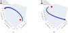 |
Fig. B.1 Isometric projection of the best-fit infalling trajectory for streamers around S CrA (left panel) and HL Tau (right panel), in 3D position– position-position space (RA, Dec, and LOS or radial distance). The black line represents the analytical trajectory from our implementation of the Mendoza et al. (2009) models, as described in Sect. 2.1. Blue spheres represent solutions from two-body REBOUND simulations (Rein & Liu 2012). The red diamonds denote the position of the center of mass of the protostellar systems. The purple circles denote the initial position of the infalling gas. These trajectories are computed up to the closest approach of infalling material to the protostellar system. |
Appendix C Distance metric
Figure C.1 illustrates computation of distance metric  , where r and θ denote the projected radial distance (from the protostar) and polar angle (with respect to the median orientation of streamer points closer than the 10th percentile of r distribution), respectively. The weighting factor (w, = 1 by default) sets the importance of rθ (distance in azimuthal direction) in the computation of distance metric. Setting w = 0, will set distance metric to be equal to the projected radial distance (r), similar to the approach by Yen et al. (2019).
Overall, a higher-value distance metric should correspond to the part of the streamer that is expected to be physically farthest away from the protostar(s). As discussed in Sect. 2.2, this distance metric is used to bin the data (for computing intensity-weighted means and standard deviations) and as an independent parameter for the final fitting.
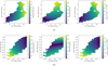 |
Fig. C.1 Computation of the distance metric (d) using polar coordinates r and θ, as discussed in Appendix C, for S CrA (top panels) and HL Tau (bottom panels). Left panels: Radial distance |


Appendix D Stellar parameters for S CrA and HL Tau
Stellar parameters used for fitting the streamers are fixed before running TIPSY, as listed for S CrA and HL Tau in Table 1. Stellar mass estimates for S CrA and HL Tau were taken from Gahm et al. (2018) and Yen et al. (2019), respectively. Distance estimate for S CrA is based on Gaia DR3 parallax value (Gaia Collaboration et al. 2023). Gaia measurements were unavailable for HL Tau, so we used the estimate of the distance to its surrounding cloud, Lynds 155 (Galli et al. 2018).
Systemic LOS velocities for S CrA A (the northern protostar) and S CrA B (the southern protostar) were inferred to be 6.07 ± 0.09 km s−1 and 5.66 ± 0.14 km s −1, respectively, using the peak of Gaussian fits to C18O (2–1) disk spectra. These C18 O (2–1) observations were part of the same ALMA project (Project Id.: 2019.1.01792.S) as the 13CO (2–1) observations discussed in Sect. 3.1. We used the mean systemic velocity of 5.86 km s−1 for the TIPSY fitting of S CrA streamer. For HL Tau, the systemic velocity derived by Yen et al. (2019) was used.
Appendix E Integrated intensity maps
Figure E.1 shows integrated intensity (moment 0) maps for 13CO (2−1) observations of S CrA and HCO+ (3−2) observations of HL Tau. The streamers are visible as the elongated gas structures.
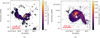 |
Fig. E.1 Integrated intensity (moment 0) maps for S CrA (left panel) and HL Tau (right panel), considering only pixels with an intensity > 3.5σ. The horizontal red lines in the bottom-left corners represent the physical length scales, and the pink ellipses in the bottom-right corners represent the beam size. Green contours in the left panel denote the continuum emission from the protoplanetary disks. |
References
- Akiyama, E., Vorobyov, E. I., Liu, H. B., et al. 2019, AJ, 157, 165 [NASA ADS] [CrossRef] [Google Scholar]
- Albrecht, S. H., Dawson, R. I., & Winn, J. N. 2022, PASP, 134, 082001 [NASA ADS] [CrossRef] [Google Scholar]
- ALMA Partnership (Brogan, C. L., et al.) 2015, ApJ, 808, L3 [Google Scholar]
- Alves, F. O., Cleeves, L. I., Girart, J. M., et al. 2020, ApJ, 904, L6 [NASA ADS] [CrossRef] [Google Scholar]
- Ankerst, M., Breunig, M. M., Kriegel, H.-P., & Sander, J. 1999, SIGMOD Rec., 28, 49 [CrossRef] [Google Scholar]
- Astropy Collaboration (Robitaille, T. P., et al.) 2013, A&A, 558, A33 [NASA ADS] [CrossRef] [EDP Sciences] [Google Scholar]
- Astropy Collaboration (Price-Whelan, A. M., et al.) 2018, AJ, 156, 123 [Google Scholar]
- Astropy Collaboration (Price-Whelan, A. M., et al.) 2022, ApJ, 935, 167 [NASA ADS] [CrossRef] [Google Scholar]
- Bae, J., Hartmann, L., & Zhu, Z. 2015, ApJ, 805, 15 [NASA ADS] [CrossRef] [Google Scholar]
- Baraffe, I., Vorobyov, E., & Chabrier, G. 2012, ApJ, 756, 118 [NASA ADS] [CrossRef] [Google Scholar]
- Bergin, E. A., Cleeves, L. I., Gorti, U., et al. 2013, Nature, 493, 644 [Google Scholar]
- Bondi, H. 1952, MNRAS, 112, 195 [Google Scholar]
- Cacciapuoti, L., Macias, E., Gupta, A., et al. 2024, A&A, 682, A61 [NASA ADS] [CrossRef] [EDP Sciences] [Google Scholar]
- Cassen, P., & Moosman, A. 1981, Icarus, 48, 353 [CrossRef] [Google Scholar]
- Chevalier, R. A. 1983, ApJ, 268, 753 [NASA ADS] [CrossRef] [Google Scholar]
- Cuello, N., Ménard, F., & Price, D. J. 2023, Eur. Phys. J. Plus, 138, 11 [NASA ADS] [CrossRef] [Google Scholar]
- Dong, R., Hall, C., Rice, K., & Chiang, E. 2015, ApJ, 812, L32 [Google Scholar]
- Dong, R., Liu, H. B., Cuello, N., et al. 2022, Nat. Astron., 6, 331 [NASA ADS] [CrossRef] [Google Scholar]
- Dullemond, C. P., Küffmeier, M., Goicovic, F., et al. 2019, A&A, 628, A20 [NASA ADS] [CrossRef] [EDP Sciences] [Google Scholar]
- Dunham, M. M., & Vorobyov, E. I. 2012, ApJ, 747, 52 [NASA ADS] [CrossRef] [Google Scholar]
- Endres, C. P., Schlemmer, S., Schilke, P., Stutzki, J., & Müller, H. S. P. 2016, J. Mol. Spectrosc., 327, 95 [NASA ADS] [CrossRef] [Google Scholar]
- Enoch, M. L., Evans, Neal J., I., Sargent, A. I., & Glenn, J. 2009, ApJ, 692, 973 [NASA ADS] [CrossRef] [Google Scholar]
- Gahm, G. F., Petrov, P. P., Tambovsteva, L. V., et al. 2018, A&A, 614, A117 [NASA ADS] [CrossRef] [EDP Sciences] [Google Scholar]
- Gaia Collaboration (Vallenari, A., et al.) 2023, A&A, 674, A1 [NASA ADS] [CrossRef] [EDP Sciences] [Google Scholar]
- Galli, P. A. B., Loinard, L., Ortiz-Léon, G. N., et al. 2018, ApJ, 859, 33 [Google Scholar]
- Garufi, A., Podio, L., Codella, C., et al. 2022, A&A, 658, A104 [CrossRef] [EDP Sciences] [Google Scholar]
- Ginski, C., Facchini, S., Huang, J., et al. 2021, ApJ, 908, L25 [NASA ADS] [CrossRef] [Google Scholar]
- Gupta, A., Miotello, A., Manara, C. F., et al. 2023, A&A, 670, L8 [NASA ADS] [CrossRef] [EDP Sciences] [Google Scholar]
- Hacar, A., Clark, S. E., Heitsch, F., et al. 2023, in Protostars and Planets VII, eds. S. Inutsuka, Y. Aikawa, T. Muto, K. Tomida, & M. Tamura, ASP Conf. Ser., 534, 153 [NASA ADS] [Google Scholar]
- Haugbølle, T., Padoan, P., & Nordlund, Å. 2018, ApJ, 854, 35 [CrossRef] [Google Scholar]
- Hennebelle, P., Lesur, G., & Fromang, S. 2017, A&A, 599, A86 [NASA ADS] [CrossRef] [EDP Sciences] [Google Scholar]
- Hsieh, T. H., Segura-Cox, D. M., Pineda, J. E., et al. 2023, A&A, 669, A137 [NASA ADS] [CrossRef] [EDP Sciences] [Google Scholar]
- Huang, J., Andrews, S. M., Öberg, K. I., et al. 2020, ApJ, 898, 140 [NASA ADS] [CrossRef] [Google Scholar]
- Huang, J., Bergin, E. A., Öberg, K. I., et al. 2021, ApJS, 257, 19 [NASA ADS] [CrossRef] [Google Scholar]
- Huang, J., Ginski, C., Benisty, M., et al. 2022, ApJ, 930, 171 [NASA ADS] [CrossRef] [Google Scholar]
- Huang, J., Bergin, E. A., Bae, J., Benisty, M., & Andrews, S. M. 2023, ApJ, 943, 107 [NASA ADS] [CrossRef] [Google Scholar]
- Jensen, S. S., & Haugbølle, T. 2018, MNRAS, 474, 1176 [Google Scholar]
- Jørgensen, J. K., Hogerheijde, M. R., Blake, G. A., et al. 2004, A&A, 415, 1021 [NASA ADS] [CrossRef] [EDP Sciences] [Google Scholar]
- Jørgensen, J. K., Schöier, F. L., & van Dishoeck, E. F. 2005, A&A, 435, 177 [NASA ADS] [CrossRef] [EDP Sciences] [Google Scholar]
- Kenyon, S. J., Hartmann, L. W., Strom, K. M., & Strom, S. E. 1990, AJ, 99, 869 [Google Scholar]
- Kuffmeier, M., Haugbølle, T., & Nordlund, Å. 2017, ApJ, 846, 7 [NASA ADS] [CrossRef] [Google Scholar]
- Kuffmeier, M., Frimann, S., Jensen, S. S., & Haugbølle, T. 2018, MNRAS, 475, 2642 [NASA ADS] [CrossRef] [Google Scholar]
- Kuffmeier, M., Dullemond, C. P., Reissl, S., & Goicovic, F. G. 2021, A&A, 656, A161 [NASA ADS] [CrossRef] [EDP Sciences] [Google Scholar]
- Kuffmeier, M., Jensen, S. S., & Haugbølle, T. 2023, Eur. Phys. J. Plus, 138, 272 [NASA ADS] [CrossRef] [Google Scholar]
- Kuznetsova, A., Hartmann, L., & Heitsch, F. 2019, ApJ, 876, 33 [NASA ADS] [CrossRef] [Google Scholar]
- Kuznetsova, A., Bae, J., Hartmann, L., & Mac Low, M.-M. 2022, ApJ, 928, 92 [NASA ADS] [CrossRef] [Google Scholar]
- Lebreuilly, U., Hennebelle, P., Colman, T., et al. 2021, ApJ, 917, L10 [NASA ADS] [CrossRef] [Google Scholar]
- Lee, J.-E., Matsumoto, T., Kim, H.-J., et al. 2023, ApJ, 953, 82 [NASA ADS] [CrossRef] [Google Scholar]
- Manara, C. F., Morbidelli, A., & Guillot, T. 2018, A&A, 618, L3 [NASA ADS] [CrossRef] [EDP Sciences] [Google Scholar]
- Manara, C. F., Ansdell, M., Rosotti, G. P., et al. 2023, in Protostars and Planets VII, eds. S. Inutsuka, Y. Aikawa, T. Muto, K. Tomida, & M. Tamura, ASP Conf. Ser., 534, 539 [NASA ADS] [Google Scholar]
- Mendoza, S., Tejeda, E., & Nagel, E. 2009, MNRAS, 393, 579 [NASA ADS] [CrossRef] [Google Scholar]
- Mercimek, S., Podio, L., Codella, C., et al. 2023, MNRAS, 522, 2384 [NASA ADS] [CrossRef] [Google Scholar]
- Mulders, G. D., Pascucci, I., Ciesla, F. J., & Fernandes, R. B. 2021, ApJ, 920, 66 [NASA ADS] [CrossRef] [Google Scholar]
- Murillo, N. M., van Dishoeck, E. F., Hacar, A., Harsono, D., & Jørgensen, J. K. 2022, A&A, 658, A53 [NASA ADS] [CrossRef] [EDP Sciences] [Google Scholar]
- Nanne, J. A. M., Nimmo, F., Cuzzi, J. N., & Kleine, T. 2019, Earth Planet. Sci. Lett., 511, 44 [CrossRef] [Google Scholar]
- Padoan, P., Kritsuk, A., Norman, M. L., & Nordlund, Å. 2005, ApJ, 622, L61 [NASA ADS] [CrossRef] [Google Scholar]
- Padoan, P., Haugbølle, T., & Nordlund, Å. 2014, ApJ, 797, 32 [Google Scholar]
- Pedregosa, F., Varoquaux, G., Gramfort, A., et al. 2011, J. Mach. Learn. Res., 12, 2825 [Google Scholar]
- Pelkonen, V. M., Padoan, P., Haugbølle, T., & Nordlund, Å. 2021, MNRAS, 504, 1219 [NASA ADS] [CrossRef] [Google Scholar]
- Pineda, J. E., Segura-Cox, D., Caselli, P., et al. 2020, Nat. Astron., 4, 1158 [NASA ADS] [CrossRef] [Google Scholar]
- Pineda, J. E., Arzoumanian, D., Andre, P., et al. 2023, in Protostars and Planets VII, eds. S. Inutsuka, Y. Aikawa, T. Muto, K. Tomida, & M. Tamura, ASP Conf. Ser., 534, 233 [NASA ADS] [Google Scholar]
- Rein, H., & Liu, S. F. 2012, A&A, 537, A128 [NASA ADS] [CrossRef] [EDP Sciences] [Google Scholar]
- Schöier, F. L., van der Tak, F. F. S., van Dishoeck, E. F., & Black, J. H. 2005, A&A, 432, 369 [Google Scholar]
- Seifried, D., Banerjee, R., Pudritz, R. E., & Klessen, R. S. 2013, MNRAS, 432, 3320 [NASA ADS] [CrossRef] [Google Scholar]
- Shariff, K., Gorti, U., & Melon Fuksman, J. D. 2022, MNRAS, 514, 5548 [NASA ADS] [CrossRef] [Google Scholar]
- Shu, F. H. 1977, ApJ, 214, 488 [Google Scholar]
- Tang, Y. W., Guilloteau, S., Piétu, V., et al. 2012, A&A, 547, A84 [NASA ADS] [CrossRef] [EDP Sciences] [Google Scholar]
- Terebey, S., Shu, F. H., & Cassen, P. 1984, ApJ, 286, 529 [Google Scholar]
- Thieme, T. J., Lai, S.-P., Lin, S.-J., et al. 2022, ApJ, 925, 32 [NASA ADS] [CrossRef] [Google Scholar]
- Thies, I., Kroupa, P., Goodwin, S. P., Stamatellos, D., & Whitworth, A. P. 2011, MNRAS, 417, 1817 [NASA ADS] [CrossRef] [Google Scholar]
- Tobin, J. J., Hartmann, L., Bergin, E., et al. 2012, ApJ, 748, 16 [Google Scholar]
- Tokuda, K., Onishi, T., Saigo, K., et al. 2018, ApJ, 862, 8 [NASA ADS] [CrossRef] [Google Scholar]
- Ulrich, R. K. 1976, ApJ, 210, 377 [Google Scholar]
- Unno, M., Hanawa, T., & Takasao, S. 2022, ApJ, 941, 154 [NASA ADS] [CrossRef] [Google Scholar]
- Valdivia-Mena, M. T., Pineda, J. E., Segura-Cox, D. M., et al. 2022, A&A, 667, A12 [NASA ADS] [CrossRef] [EDP Sciences] [Google Scholar]
- Virtanen, P., Gommers, R., Oliphant, T. E., et al. 2020, Nat. Methods, 17, 261 [Google Scholar]
- Visser, R., van Dishoeck, E. F., Doty, S. D., & Dullemond, C. P. 2009, A&A, 495, 881 [NASA ADS] [CrossRef] [EDP Sciences] [Google Scholar]
- Vorobyov, E. I., & Basu, S. 2005, ApJ, 633, L137 [NASA ADS] [CrossRef] [Google Scholar]
- Vorobyov, E. I., Skliarevskii, A. M., Elbakyan, V. G., et al. 2020, A&A, 635, A196 [NASA ADS] [CrossRef] [EDP Sciences] [Google Scholar]
- Welch, W. J., Hartmann, L., Helfer, T., & Briceño, C. 2000, ApJ, 540, 362 [NASA ADS] [CrossRef] [Google Scholar]
- Yen, H.-W., Takakuwa, S., Ohashi, N., et al. 2014, ApJ, 793, 1 [NASA ADS] [CrossRef] [Google Scholar]
- Yen, H.-W., Takakuwa, S., Chu, Y.-H., et al. 2017, A&A, 608, A134 [NASA ADS] [CrossRef] [EDP Sciences] [Google Scholar]
- Yen, H.-W., Koch, P. M., Manara, C. F., Miotello, A., & Testi, L. 2018, A&A, 616, A100 [NASA ADS] [CrossRef] [EDP Sciences] [Google Scholar]
- Yen, H.-W., Gu, P.-G., Hirano, N., et al. 2019, ApJ, 880, 69 [NASA ADS] [CrossRef] [Google Scholar]
- Zhang, Y., Ginski, C., Huang, J., et al. 2023, A&A, 672, A145 [NASA ADS] [CrossRef] [EDP Sciences] [Google Scholar]
All Tables
All Figures
|
Fig. 1 Schematic diagram of coordinate axes used to compute the theoretical trajectories of infalling gas (green cloud) around a protostellar system (orange star), as discussed in Sect. 2.1. |
| In the text | |
|
Fig. 2 Flow of S CrA 13CO (2–1) data in the TIPSY pipeline. Panel a: intensity-weighted velocity (moment 1) map in colors, overlaid with contours representing the integrated intensity (moment 0; see Fig. E.1). The red segments in the bottom-left corners depict a length scale of 1000 au. The pink ellipses in the bottom-right corners depicts the beam size of the data. Panel b: isometric projection of the 3D PPV diagram of pixels with intensity >5σ in the whole field of view. Panel c: isometric projection of the PPV diagram of an isolated and cleaned streamer. The red square and its error bars represent intensity-weighted means and standard deviations, respectively. Panel d: same as panel c, but with the best-fit trajectory, as represented by the black line. Black circles denote the interpolated values of the theoretical trajectory, which are directly compared to the intensity-weighted means. Panel e: same as panel b, but with the best-fit trajectory, as represented by the black line. 3D interactive versions of panels d and e are available online. |
| In the text | |
|
Fig. 3 Same procedure as described in Fig. 2, but for HL Tau instead of S CrA. 3D interactive versions of panels d and e are available online. |
| In the text | |
|
Fig. 4 Distribution of goodness-of-fit estimates as functions of free parameters: initial speed on the POS (x-axis) and initial spatial offset in the LOS direction, for TIPSY fitting for S CrA (top panels) and HL Tau (bottom panels). Here, initial direction of gas in the POS (third free parameter) is fixed to the value for the best fit. Left panels: distribution of fractions of coordinate values of points in the observed streamer curve (intensity-weighted means and standard deviations), which is consistent with the theoretical trajectories. Right panels: distribution of log(log(χ2)) deviations between the observed streamer curve and theoretical trajectories. In all the plots, yellow regions represent good fits. Red squares represent the best fit, as discussed in Sect. 2.2. The red lines passing through them represent errors, as discussed in Sect. 2.3. |
| In the text | |
|
Fig. B.1 Isometric projection of the best-fit infalling trajectory for streamers around S CrA (left panel) and HL Tau (right panel), in 3D position– position-position space (RA, Dec, and LOS or radial distance). The black line represents the analytical trajectory from our implementation of the Mendoza et al. (2009) models, as described in Sect. 2.1. Blue spheres represent solutions from two-body REBOUND simulations (Rein & Liu 2012). The red diamonds denote the position of the center of mass of the protostellar systems. The purple circles denote the initial position of the infalling gas. These trajectories are computed up to the closest approach of infalling material to the protostellar system. |
| In the text | |
|
Fig. C.1 Computation of the distance metric (d) using polar coordinates r and θ, as discussed in Appendix C, for S CrA (top panels) and HL Tau (bottom panels). Left panels: Radial distance |
| In the text | |
|
Fig. E.1 Integrated intensity (moment 0) maps for S CrA (left panel) and HL Tau (right panel), considering only pixels with an intensity > 3.5σ. The horizontal red lines in the bottom-left corners represent the physical length scales, and the pink ellipses in the bottom-right corners represent the beam size. Green contours in the left panel denote the continuum emission from the protoplanetary disks. |
| In the text | |
Current usage metrics show cumulative count of Article Views (full-text article views including HTML views, PDF and ePub downloads, according to the available data) and Abstracts Views on Vision4Press platform.
Data correspond to usage on the plateform after 2015. The current usage metrics is available 48-96 hours after online publication and is updated daily on week days.
Initial download of the metrics may take a while.