| Issue |
A&A
Volume 683, March 2024
|
|
|---|---|---|
| Article Number | A142 | |
| Number of page(s) | 12 | |
| Section | Astronomical instrumentation | |
| DOI | https://doi.org/10.1051/0004-6361/202347960 | |
| Published online | 15 March 2024 | |
Extended scene deep-phase-retrieval Shack-Hartmann wavefront sensors
1
Key Laboratory of Adaptive Optics, Chinese Academy of Sciences,
Chengdu
610209, PR China
e-mail: This email address is being protected from spambots. You need JavaScript enabled to view it.
2
Institute of Optics and Electronics, Chinese Academy of Sciences,
Chengdu
610209, PR China
e-mail: This email address is being protected from spambots. You need JavaScript enabled to view it.
; This email address is being protected from spambots. You need JavaScript enabled to view it.
3
The University of Chinese Academy of Sciences,
Beijing
100049, PR China
Received:
14
September
2023
Accepted:
22
January
2024
Abstract
Context. Strong atmospheric turbulence has been a challenge for high-resolution imaging of solar telescopes. Adaptive optics (AO) systems are capable of improving the quality of imaging by correcting partial aberrations. Thus, the performance of Shack-Hartmann sensors in measuring aberrations generally determines the upper performance bound of AO systems. In solar AO, classic correlation Shack-Hartmann sensors only correct a small number of modal aberrations. Moreover, strong aberrations are difficult to measure stably by correlation Shack-Hartmann. In this context, the improvement in the performance of Shark-Hartmann sensors promises to enable higher-resolution imaging of extended objects for ground-based telescopes or Earth observation.
Aims. We propose a new extended scene deep-phase-retrieval Shack-Hartmann wavefront sensing approach to improve the image quality of solar telescopes. It is capable of achieving high-accuracy measurements of high-spatial-resolution wavefronts on extended scene wavefront sensing. Moreover, it has great generalization when observing unknown objects from different fields of view of the telescope.
Methods. Our proposed approach can extract features resembling the sub-aperture point spread function (PSF) from a Shack-Hartmann sensor image without any prior information. Then a convolutional neural network is used to establish a nonlinear mapping between the feature image and the wavefront modal coefficients. The extracted feature greatly eliminates the shape information of the extended object while maintaining more information related to aberrations. We verified the performance of the proposed method through simulations and experiments.
Results. In the indoor experiment on the ground layer adaptive optics (GLAO) of the 1 m New Vacuum Solar Telescope, compared to the Shack-Hartmann correlation method, the proposed method reduces the correction errors by more than one third. When observing objects from different fields of view in the GLAO that differ from the object in the training data, the relative errors fluctuate within the range of 20% to 26%. The AO system with the proposed wavefront measurement method can obtain higher-resolution focal images of the simulated solar granulation after a round of offline correction. The average latency of the proposed method is about 0.6 ms.
Key words: turbulence / atmospheric effects / instrumentation: adaptive optics / instrumentation: high angular resolution / techniques: high angular resolution / techniques: image processing
© The Authors 2024
 Open Access article, published by EDP Sciences, under the terms of the Creative Commons Attribution License (https://creativecommons.org/licenses/by/4.0), which permits unrestricted use, distribution, and reproduction in any medium, provided the original work is properly cited.
This article is published in open access under the Subscribe to Open model. This email address is being protected from spambots. You need JavaScript enabled to view it. to support open access publication.
1 Introduction
The adaptive optics (AO) system has already been used in various applications, such as ground-based telescopes (Rao et al. 2016; Kim et al. 2021; Guo et al. 2016) and biological imaging (Booth 2014; Zhou et al. 2022; Guo et al. 2022b). It plays an important role in high-resolution imaging (Oberti et al. 2022) by correcting aberrations caused by atmospheric turbulence or biological tissue. Some astronomers began to use the Shack-Hartmann wavefront sensor (SHWFS) in the late 1970s for testing large telescope optics (Tyson & Frazier 2022). SHWFS consists of two parts, a microlens array and a CCD sensor. The microlens array divides the wavefront into small sub-wavefronts. The SHWFS indirectly measures the wavefront inside its pupil by utilizing the imaging information of each sub-wavefront on the CCD.
Over the course of several decades, wavefront sensing methods based on the SHWFS have been developed. The most classical method, called the slope-based method, reconstructs the aberration coefficients by multiplying the slopes with the reconstruction matrix. Further research has suggested utilizing additional features to reconstruct the wavefront by introducing more comprehensive information, such as the slopes of the spot in other directions besides the horizontal and vertical (Rouzé et al. 2021), as well as first-order and second-order moments (Viegers et al. 2017; Feng et al. 2018). To avoid the limitations of slope features when applied to wavefront measurements, some studies have proposed iteratively calculating the aberration directly from SHWFS images instead of calculating the slope features (Li et al. 2014; Brunner et al. 2017), but this type of method is time-consuming and has poor convergence. In recent years, the rapid advancement of artificial intelligence has led to the emergence of wavefront sensing methods that integrate neural networks. These methods have performed impressively in wavefront reconstruction (DuBose et al. 2020; Wu et al. 2020; Zuo et al. 2022). For example, a deep-phase-retrieval wave-front reconstruction (DPRWR) method was proposed by our group in a previous work, and utilizes convolutional neural networks (CNNs) and full connection layers to establish a mapping between point-source SHWFS spot images and Zernike modal coefficients (Guo et al. 2022a). Experiments confirmed that Zernike modal coefficients for two to six times the number of sub-apertures can be measured by DPRWR with high precision (Zhang & Guo 2023). Compared with the slope-based method, in which the number of Zernike modal coefficients at most achieve 0.6–0.8 times the number of sub-apertures (Rao et al. 2016; Denker et al. 2007), the spatial resolution and measurement accuracy in DPRWR have been greatly improved.
However, when the light source or observed object is an extended object, the shape of the extended object and the sub-aperture point spread function (PSF) will undergo convolution effects on the sensor, while the SHWFS image formed by a point source is the sub-aperture PSF in its own right. Therefore, point-source wavefront reconstruction methods cannot be directly applied to extended objects. In solar telescopes or Earth observation, the correlation SHWFS is commonly used to measure wavefronts (Smithson & Tarbell 1977; Von Der Lühe 1983; Endo et al. 2019). It calculates the displacement of each sub-aperture image relative to a reference sub-aperture image through correlation operations, by which the aberration coefficients can be obtained by multiplying the reconstruction matrix. The correlation SHWFS and the centroid slope-based method are essentially similar, both establishing a linear mapping relationship between slope features and aberrations. Therefore, the correlation SHWFS also suffers from similar limitations caused by slope features, such as the inability to achieve high-spatial-resolution wavefront measurements and a weak fitting capability. For example, in this research (Endo et al. 2019), the correlation SHWFS achieves an accuracy measurement of less than 0.04 λ for only the fifth-order aberration at a specific sensor parameter. The ground layer adaptive optics (GLAO) of the 1 m New Vacuum Solar Telescope (NVST) at Fuxian Solar Observatory in China can measure the first 45 Zernike modes with the correlation SHWFS (Zhang et al. 2023b). The difference between the correlation SHWFS and the centroid slope-based method is that the correlation SHWFS to some extent eliminates the interference of object shape with wavefront estimation. This approach, calculating features that are independent of the object’s shape and strongly correlated with aberrations, can be considered as a way to apply point-source wavefront reconstruction methods to extended scenes. However, in the presence of strong turbulence, the sub-aperture objects are distorted and blurred, which may result in a significant decrease in the accuracy of calculations related to the corresponding slopes and in turn affect the accuracy of wavefront measurement. Similar to the correlation SHWFS, de Bruijne et al. (2022) proposed a method using a semi-blind deconvolution algorithm to recover the PSF image from the extended scene SHWFS image and then reconstruct the wavefront phase screen using a UNet network. This method is time-consuming due to iterative calculation, and it requires a higher-resolution object image as the initial value for the blind deconvolution iteration. The method proposed by Xin et al. (2019) is to extract a PSF-like image from a pair of phase diversity images and is capable of measuring the 2nd–37th Zernike modal coefficients.
In recent years, computers have become extremely powerful in terms of computational capabilities, which means they can handle the enormous computational demands of neural networks. Thus, deep learning algorithms can be endowed with remarkable learning abilities that were previously unimaginable. Concomitantly, another class of extended scene wavefront sensing methods emerged, which directly establishes a mapping between extended scene images and aberrations. Nishizaki et al. (2019) construct CNNs to reconstruct the wavefront from a single intensity image. Riesgo et al. (2022) construct a fully convolutional neural network to reconstruct the wavefront directly from simulated solar granulation SHWFS images. For this type of method, despite the fact that neural networks can still converge well with appropriate parameters in their datasets, generalization remains a challenging issue (Zhang et al. 2023a). This is because the mapping learned by neural networks cannot break free from its reliance on the current object shape. When the observed object changes, new images need to be collected and the network needs to be retrained.
This paper proposes a new SHWFS feature image extraction method whereby the extracted feature images are obtained by some frequency-domain computation processes on a single SHWFS image. Then we construct a neural network to reconstruct the wavefront from the feature images that are similar to the PSF and independent of the shapes of extended objects. In this paper, we refer to this method as an extended scene deep-phase-retrieval wavefront reconstruction method (ES-DPRWR) for Shack-Hartmann wavefront sensors. ES-DPRWR is capable of achieving high-precision measurements of high-spatial-frequency aberrations and great generalization, which is sufficiently demonstrated in the subsequent simulations and experiments.
Four more sections make up this manuscript. The methods section consists of an introduction to the principle of the traditional correlation SHWFS, a theoretical analysis of feature image extraction, and a presentation of the structure of the used neural network. The simulation scheme, results, and some discussion are presented in Sect. 3. The experimental platform, the GLAO on the NVST, and some comparative experiments on this platform are detailed in Sect. 4. Finally, conclusions and future development are presented in Sect. 5.
2 Methods
2.1 Correlation SHWFS
In solar AO, the wavefront of the light from the solar surface is reconstructed by calculating the correlation slopes of the sub-aperture images acquired by the SHWFS. It is essential for this method to select a sub-aperture image as a reference image Ir(k, l). The cross-covariance (Von Der Lühe 1983) C(x, y) of each sub-aperture is given by
 (1)
(1)
where I(x, y) is the sub-aperture image. The correlation slopes, gx and gy, of each sub-aperture in the horizontal and vertical directions, respectively, are as follows:
 (2)
(2)
 (3)
(3)
where (xc, yc) are the coordinates of the peak in the cross-covariance image, C(x, y), and (x0, y0) are the coordinates of the centroid of mass in the spot image with no aberration. The correlation SHWFS assumes that the correlation slope vector, g, and the Zernike modal coefficients, z, have a linear mapping:
 (4)
(4)
where g contains slopes gx and gy of all sub-apertures. To obtain the reconstruction matrix, D−1, the correlation slopes per root mean square (RMS) single-order aberration at different spatial frequencies are measured as follows:
![Mathematical equation: $\left[ {\matrix{ {{G_{x1}}\left( 1 \right)} & {{G_{x2}}\left( 1 \right)} & \cdots & {{G_{xn}}\left( 1 \right)} \cr {{G_{y1}}\left( 1 \right)} & {{G_{y2}}\left( 1 \right)} & \cdots & {{G_{yn}}\left( 1 \right)} \cr {{G_{x1}}\left( 2 \right)} & {{G_{x2}}\left( 2 \right)} & \cdots & {{G_{xn}}\left( 2 \right)} \cr {{G_{y1}}\left( 2 \right)} & {{G_{y2}}\left( 2 \right)} & \cdots & {{G_{yn}}\left( 2 \right)} \cr \cdots & \cdots & \cdots & \cdots \cr {{G_{x1}}\left( m \right)} & {{G_{x2}}\left( m \right)} & \cdots & {{G_{xn}}\left( m \right)} \cr {{G_{y1}}\left( m \right)} & {{G_{y2}}\left( m \right)} & \cdots & {{G_{yn}}\left( m \right)} \cr } } \right] = D \cdot \left[ {\matrix{ 1 & \cdots & 0 \cr \vdots & \ddots & \vdots \cr 0 & \cdots & 1 \cr } } \right],$](/articles/aa/full_html/2024/03/aa47960-23/aa47960-23-eq5.png) (5)
(5)
where, for example, Gx1(2) and Gy1(2) represent the correlation slopes in the x and y directions per the RMS first-order aberration at the second sub-aperture, respectively. In Eq. (5), m represents the number of effective sub-apertures, and n represents the number of aberration modes. The above equation can be denoted as
 (6)
(6)
where E is the identity matrix. Thus, D−1 can be solved by singular value decomposition:
 (7)
(7)
Finally, the reconstructed phase is the summation of the Zernike polynomials multiplied by the corresponding modal coefficients,
 (8)
(8)
where φk(x, y) is the kth-order Zernike polynomial, zk is the modal coefficient of the kth-order Zernike polynomial, and n is the total number of coefficients.
2.2 ES-DPRWR
The extended scene deep-phase-retrieval wavefront reconstruction method proposed in this manuscript reconstructs aberrations using feature images extracted from SHWFS images by neural networks rather than directly based on SHWFS images. Therefore, ES-DPRWR consists of two steps. One is to filter out the shape information of the object from the acquired SHWFS image as well as to extract a feature image that retains only the aberration information; the theoretical principle of this preprocessing is presented in Sect. 2.2.1. The second step is to feed a feature image into the network so as to predict the corresponding Zernike coefficients of the aberration; the architecture of the network used in this manuscript is presented in Sect. 2.2.2.
2.2.1 Method to extract feature images
For the SHWFS, each sub-aperture image is formed by the light coming from different directions to an object. It was assumed that the object in the field of view of each sub-aperture was the same for the method of extracting feature images in this paper.
Based on the theory of Fourier optics, each sub-aperture image, Ii, can be seen as the convolution between the extended object, O, and the PSF of the corresponding sub-aperture:
 (9)
(9)
where i represents the order of the sub-aperture, and where the two-dimensional convolution process is represented by **.
The convolution operation can be Fourier-transformed on both sides, as is shown in Eq. (10), where the Fourier transform is represented by ℱ:
 (10)
(10)
Similarly, a sub-aperture image is selected as the reference sub-aperture image, I0. Then, each one of the Fourier-transformed sub-aperture images and the Fourier-transformed reference sub-aperture image are divided at corresponding pixels, as is shown in Eq. (11), where ℱ(O)ℱ (PSFi) presents the dot product between ℱ(O) and ℱ (PSFi). This step theoretically eliminates the information about the extended object and only the information related to aberrations remains:
 (11)
(11)
The inverse Fourier transform of the value after the division is the sub-aperture feature image, Ki:
 (12)
(12)
Thus, a sub-aperture feature image can be obtained by the above steps for each sub-aperture of the SHWFS from a single SHWFS image. All the sub-aperture feature images are stitched together into an SHWFS feature image according to the layout of the microlens array. The ES-DPRWR method proposed in this paper aims to reconstruct the mapping from the SHWFS feature image that is independent of the extended object to the modal coefficients of the wavefront by neural networks.
However, as is seen in Eq. (11), this step introduces a disturbing factor, PSF0, the aberration of the reference sub-aperture, into an SHWFS feature image, while eliminating the extended object information. The feature image varies with different PSF0 when selecting different reference sub-apertures, which makes the fitting of the mapping more difficult and affects the generalization of ES-DPRW. Ideally, when the PSF0 of the reference sub-aperture image is close enough to the Airy disk, the sub-aperture feature image can be maximized to avoid the interference of this factor. In the experiment, to approach this point as closely as possible, the reference sub-aperture image was preferably the sub-aperture image with the minimum aberration of all the sub-apertures. In Figs. 1 and 2, we verified the negative correlation between both, the Strehl ratio (SR) of the focal spot image and the contrast of the focal extended object image, and the magnitude of aberration by simulation experiments. For the first 299 aberration modes, each single-order aberration within the range of (−1, 1) rad maintains a strong negative correlation between its magnitude and image contrast. In Fig. 1, we only list the mapping curves for the 3rd, 20th, 65th, 135th, 230th, and 275th aberration modes. Moreover, for aberrations conforming to the atmospheric turbulence distribution, as the D/r0 increases, the aberration distortion becomes more drastic, and the statistical contrast of the focal extended object image becomes smaller. Thus, in experiments, we selected an extended scene sub-aperture image with the highest contrast of all the sub-apertures as a reference sub-aperture image for the corresponding SHWFS image.
In addition, another disturbing factor, periodic noises with various frequencies, will appear in the feature image when a heavily distorted sub-aperture image is selected as a reference image. The influence of the aberration on the object image means the loss of high-frequency information, which will lead to the generation of a few extremely small values in the high-frequency region of the frequency spectrogram of the reference sub-aperture image. In Eq. (12), these small values of ℱ (I0) will become extremely large values in turn after the division of the ℱ(Ii) and ℱ(I0). They are eventually Fourier-transformed to periodic high-frequency noise in the feature image, Ki. Stronger phase distortion in the reference sub-aperture image will result in more high-frequency noises. This is one of the reasons why the reference sub-aperture image with the minimum aberration should be selected. But the aberration of the reference sub-aperture is still unavoidable. Thus, it is necessary to have some strategies to suppress noise. In this paper, we took these two steps, including adding a regularization to the frequency spectrogram of the reference sub-aperture image and designing notch filters for the ℱ(Ii)/ℱ(I0).
The performance of the above three strategies in noise reduction and noise filtering on the feature image is confirmed in the following experiment, which ensures the high accuracy and generalizability of the ES-DPRWR adopting the feature image. The completed computational flow of feature image extraction is shown in Fig. 3.
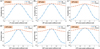 |
Fig. 1 Negative correlation between both the SR of the focal spot image and the contrast of the focal extended object image, and the magnitude of the single-order modal aberration. Panels a–f show the mapping curves with respect to the 3rd, 20th, 65th, 135th, 230th, and 275th modal aberrations, respectively. For each panel, all the values in the “SR” curve were normalized by dividing by their maximum SR, and similarly all the values in the “Contrast” curve were normalized by dividing by their maximum contrast. |
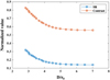 |
Fig. 2 Negative correlation between the SR of the focal spot image, the contrast of the focal extended scene image, and the magnitude of the atmospheric turbulence aberration. The value of each point is the average of the contrast of 1000 focal object images under 1000 random aberrations with corresponding D/r0. |
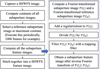 |
Fig. 3 Computational flow of feature image extraction. |
2.2.2 Network architecture
As is shown in Fig. 4, first, an SHWFS feature image that is the same size as the SHWFS image will be obtained according to the formulations in Sect. 2.2.1. The SHWFS feature image is then fed into the ES-DPRWR network, which eventually outputs the reconstructed modal coefficients. The network of the ES-DPRWR is the same as the network used in previous research about DPRWR, which has been detailed in previous research (Guo et al. 2022a). Subsequent experiments demonstrate that this network has a good performance in the study to reconstruct the modal coefficients from PSF-like SHWFS feature images.
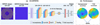 |
Fig. 4 Schematic diagram of the ES-DPRWR method. (a) The structure of the ES-DPRWR network. (b) The reconstructed wavefront and the true wavefront. |
2.3 Evaluation metrics
The error between the estimated wavefront and the true wave-front directly indicates the accuracy of the wavefront reconstruction method. When the aberrations are represented by Zernike polynomials, the root mean square error (RMSE) of the wavefront is equivalent to the RMSE of the Zernike modal coefficients:
 (13)
(13)
where  represents an estimated Zernike coefficient and zk represents a true Zernike mode coefficient.
RMSE is an absolute accuracy, and the relative error provides a more intuitive comparison of the performance in wave-front reconstruction of the different methods. The relative error, Erel, is obtained by dividing the RMSE by the RMS of the true wavefront:
 (14)
(14)
Generally, the contrast (Wang et al. 2021) is used to assess the degree of distortion in extended object images. It is calculated by the following formulation:
![Mathematical equation: $C = {{\sum\nolimits_{k = 1}^S {\,{{\left[ {I\left( {x,y} \right) - \bar I} \right]}^2}} } \over {\sum\nolimits_{k = 1}^S {\,I{{\left( {x,y} \right)}^2}} }},$](/articles/aa/full_html/2024/03/aa47960-23/aa47960-23-eq16.png) (15)
(15)
where S is the number of pixels of the image, I(x, y), and Ī is the mean of this image.
3 Numeric simulation
One of the most important steps in our proposed method is the extraction of feature images. Section 3.1 shows the similarity between the simulated feature image after stripping the object information and the PSF of the aberration. This is the reason why ES-DPRWR has great generalizability when observing different targets. In order to powerfully demonstrate the independence of the proposed method from the observed object, the ES-DPRWR network was trained on the set of feature images obtained from point-source SHWFS images and the trained network was tested on feature images obtained from extended object SHWFS images. The performance of the trained ES-DPRWR network, which is absolutely unrelated to extended objects in the extended scene wavefront reconstruction, is shown in Sect. 3.2.
Parameters of the SHWFS.
3.1 Feature images and simulation datasets
The training dataset of the ES-DPRWR network consisted of 100000 feature images for point-source SHWFS images and 299 corresponding Zernike modal coefficients that conform to D/r0 = 24. The simulation principle and steps of the point-source SHWFS images have been described in previous research work (Zhang & Guo 2023). The parameters of the SHWFS used in this simulation experiment are shown in Table 1.
In addition, we simulated three test sets of SHWFS images with the same aberrations while the objects were point sources, two solar granulations, respectively. First, we selected two different regions in a simulated high-resolution solar granulation image (Fig. 5a) and undertook down-sampling (Figs. 5b, c) for the simulation of solar granulation SHWFS images. Then, we obtained three test datasets of feature images by means of the computational method in Sect. 2.2.1.
Six examples of these test sets of images are respectively seen in Figs. 6a–f. As is visualized in this figure, a sub-aperture feature image for a point-source spot image stays as a spot image, while a sub-aperture feature image for a solar granulation loses the shape information that can be seen in the solar granulation SHWFS image. Seven sub-apertures were randomly selected to carefully compare sub-aperture feature images on a point source, solar granulation 1 and solar granulation 2, as is seen in Fig. 6g. It can be observed that the shape of spots in the sub-aperture feature images for the two solar granulations is quite similar to that of spots in the corresponding sub-aperture feature images for the point source, which intuitively verifies the independence of the extended scene feature image from the shape of objects. The residual images of SHWFS feature images for the point source and solar granulations are shown in Fig. 7. The means of the grayscale of two residual images are 4.4e−4 and 1.3e−3, respectively, which are only one thousandth or so the magnitude of feature images.
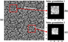 |
Fig. 5 Original solar granulation image and two down-sampled solar granulation images. The size of a sub-aperture image is 20 × 20 in this simulation. Thus, two original solar granulations boxed in red in panel a are down-sampled to panels b and c to satisfy the sub-aperture field of view. |
RMSE of Zernike coefficients for the correlation SHWFS with different numbers of the reconstructed modes.
3.2 Results
The accuracy of wavefront measurements for both ES-DPRWR and correlation SHWFS are compared in this subsection.
First, the optimal number of reconstructed modes for the correlation SHWFS can be selected from Table 2, where the RMSE of Zernike modal coefficients for the correlation SHWFS is the smallest. The test data for Table 2 are the sets of 1000 SHWFS images for the solar granulation. In the subsequent Tables 3 and 4, the correlation SHWFS reconstructs the 3rd–105th Zernike modal coefficients and the unreconstructed modal coefficients are considered to be zero, while ES-DPRWR is capable of reconstructing the 3rd–299th Zernike modal coefficients.
Furthermore, the performance of the ES-DPRWR and correlation SHWFS are compared, as is shown in Table 3 and Fig. 8. For the ES-DPRWR method, the RMSE and the relative error of the measured wavefront in the point-source SHWFS feature image are 0.107 λ and 13.4%, respectively, and those in the SHWFS feature images for the two solar granulations are 0.164 λ and 20.5%, 0.115 λ and 14.4%, respectively. It can be noted that the measurement errors for the ES-DPRWR trained on the point-source dataset when testing the two different solar granulation datasets increased by 7.1% and 1.0%, respectively, compared to the point-source test dataset. However, they both still drop by at least one third of the errors measured by the correlation SHWFS. This demonstrates the feasibility of the ES-DPRWR for the accurate measurement of modal coefficients when observing unknown objects. We randomly selected a frame of the measured aberration for a visual comparison. Residual wavefronts for the two methods are shown in Fig. 8. The RMSs of residual wavefronts for ES-DPRWR are all smaller than those of the traditional correlation SHWFS.
Moreover, we tested the performance of the ES-DPRWR at various degrees of aberration distortion. As D/r0 increases from 13 to 36, the distortion of aberrations becomes more and more drastic and the statistical RMS of the wavefront gradually increases from 0.478 λ to 1.119 λ. In Fig. 9, RMSEs for the ES-DPRWR slowly rise as aberrations get larger, while fluctuations of relative errors maintain within approximately 7%. It can be confirmed that the ES-DPRWR provides a wide measurable range of aberrations and possesses the potential to measure strong aberrations. This is supported by a smart normal distribution of aberrations at D/r0 of 24 in the training dataset. It contains a total of 100 000 frames of aberrations, of which 63% get D/r0 concentrated between 18–29, 30% are distributed between 13–17, 30–36, and the rest are distributed outside of this.
Comparison of RMSEs (λ) and relative errors of 3rd–299th Zernike coefficients for two methods.
4 Experimental verification
In the above simulation experiments, it is preliminarily demonstrated that the ES-DPRWR method can reconstruct wavefronts with a higher accuracy and higher spatial resolution. This section shows the test results of the ES-DPRWR method on the GLAO of the NVST at Fuxian Solar Observatory in China. ES-DPRWR still performs well in this experiment.
4.1 Introduction of GLAO to the NVST
Ground layer adaptive optics aims to correct aberrations across a wide field of view for large ground-based optical telescopes (Schmidt et al. 2017; Yang et al. 2023). The GLAO on the NVST is a 151-element AO system (as is shown in Fig. 10), where the SHWFS is a multidirectional SHWFS (MD-SHWFS) that detects the wavefront aberrations from different lines of sight simultaneously. This wavefront sensor utilizes a hexagonal microlens array arranged in a 9 × 8 grid, as is seen in Fig. 11. The field of view for wavefront sensing is 42″ × 37″, which is divided into nine guide star (GS) regions in a 3 × 3 grid, as is shown in Fig. 12.
When acquiring the training dataset, a simulated solar granulation image with a high resolution was placed at the focal plane of the telescope. The deformable mirror (DM) simulated 30 000 frames of random aberrations at D/r0 = 10 composed of 77th-order Zernike modal aberrations. 30 000 corresponding frames of MD-SHWFS images were captured frame by frame. Only the feature images extracted from the SHWFS images in the fifth GS region were used to train the ES-DPRWR network in this experiment. The labels are the 77th-order Zernike modal coefficients. The DM simulated a new frame of random aberration at D/r0 = 10 and a MD-SHWFS image was captured. The trained ES-DPRWR network reconstructed the wavefront modal coefficients from the feature image extracted from that MD-SHWFS image. A group of voltages could be obtained by multiplying a 77th-order Zernike modal voltage matrix by modal coefficients. Then the current voltage minus the measured voltage was fed into the DM. Thus, restored focal images of the simulated solar granulation could be observed on the focal camera.
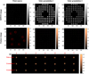 |
Fig. 6 Examples of SHWFS images and feature images with the same aberration. Panels d–f show the feature images of corresponding SHWFS images, panels a–c, respectively. In order to compare these three feature images more clearly, the sub-aperture feature images boxed in red in panel d are shown in the first row of panel g, respectively. The second and third rows in panel g show the corresponding sub-aperture feature images in panels e and f, respectively. |
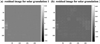 |
Fig. 7 Two residual images. Panel a shows the residuals of the solar granulation 1 feature image (Fig. 6e) and the point-source feature image (Fig. 6d). Panel b shows the residuals of the solar granulation 1 feature image (Fig. 6f) and the point-source feature image (Fig. 6d). |
Measurement errors for ES-DPRWR and correlation SHWFS in the experiment.
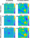 |
Fig. 8 Comparison of residual wavefront phase screens of ES-DPRWR and correlation SHWFS. |
4.2 Performance comparison
The ES-DPRWR and correlation SHWFS with different reconstruction matrices of 20, 27, 35, 39, and 41 orders, respectively, estimated the wavefront in the fifth GS region from the test datasets. The RMSEs of the wavefront reconstructed by these two methods are shown in Table 4, where each value in the table is the average of 100 groups of test data. When the number of reconstructed Zernike modes is 35, the RMSE and the relative error for the correlation SHWFS are the smallest, 0.1287 λ and 36%, respectively, while those for ES-DPRWR are 0.071 λ and 20%. Compared to the optimal correlation SHWFS, the spatial resolution of ES-DPRWR is approximately doubled, from 35 orders to 77 orders, and the accuracy improves by 0.0577 λ.
The focal images recovered by ES-DPRWR and the correlation SHWFS are compared, as is shown in Fig. 13. Figures 13a–f include the original focal image, recovered focal images, residual wavefronts, and true wavefront with an RMS of 0.563 λ. The contrast of the original focal image disturbed by aberration is only 0.027 and the details of the solar granulation are pretty blurry. The contrast of the focal images recovered by ES-DPRWR and the correlation SHWFS increases to 0.118 and 0.058, respectively. It is obvious that the performance of the ES-DPRWR is better. The resolution of the focal image recovered by ES-DPRWR is higher compared with the correlation SHWFS. The RMSE of the wavefront reconstructed by ES-DPRWR is 0.084 λ smaller than that of the wavefront reconstructed by the correlation SHWFS. For a small aberration, as is seen in Figs. 13g–l, the ES-DPRWR still outperforms the traditional correlation SHWFS.
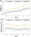 |
Fig. 9 Performance of the ES-DPRWR network trained on the dataset at D/r0=24 when measuring aberrations at D/r0 of 13–36 for the point source, granulation 1 and granulation 2, respectively. (a) RMSEs. (b) Relative errors. |
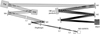 |
Fig. 10 Optical layout of GLAO on the 1-meter NVST (Zhang et al. 2023b). |
RMSEs and relative errors of modal coefficients reconstructed by ES–DPRWR on nine different GSs.
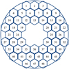 |
Fig. 11 Arrangement of the sub-apertures in the MD-SHWFS. |
4.3 Generalization comparison
The different regions of nine GSs in the sub-aperture image are shown in Fig. 12. The details of the solar granulation in different GS regions are different. In the GLAO on the NVST, the pupil plane of the MD-SHWFS and the plane where the DM is located are conjugated to each other. The lights coming from different directions form images on nine GS regions in the focal plane. Thus, the distorted phase screens in the nine GS regions are consistent with the phase imposed by the DM.
The ES-DPRWR network only trained on the set of the feature images for GS 5 can reconstruct nine different groups of Zernike modal coefficients for these nine GSs. The RMSEs for nine groups of reconstructed wavefronts are shown in Table 5.
The RMSEs of 3rd–77th Zernike modal coefficients of the nine regions fluctuate between 0.071 λ and 0.092 λ, with relative errors ranging from 20% to 26%. For low-order aberrations (3rd–35th), the RMSEs fluctuate between 0.058 λ and 0.079 λ, with relative errors ranging from 17% to 23%; for high-order aberrations (36rd–77th), the RMSEs fluctuate between 0.045 λ and 0.056 λ, with relative errors ranging from 37% to 50%. It can be seen that the ES-DPRWR network, which is independent of objects in the other eight regions, still performs well on wavefront measurement for the other eight fields of view.
To further demonstrate the advantages of our approach in terms of generalization, we compared the performance of the ES-DPRWR network and the method of Riesgo et al. (2022). Riesgo’s network was directly trained on the solar granulation SHWFS images. The training datasets of the two networks are both from the GS 5 region in the SHWFS images. The measurement accuracies of these two methods for different GSs are shown in Table 6. For GS 5, the RMSE and the relative error for ES-DPRWR are 0.071 λ and 20%, respectively, while for Riesgo’s network they are 0.052 λ and 14%, respectively. For GS 1 and GS 9, the RMSEs and the relative errors for ES-DPRWR increase slightly, namely to 0.089 λ and 25%, and 0.078 λ and 22%, respectively; while for Riesgo’s network they all increase dramatically, namely to 0.344 λ and 96%, and 0.369 λ and 103%, respectively. According to the above experimental results, it is confirmed that Riesgo’s network has a slight accuracy advantage when observing the object that is the same as the training data. This is because the feature images inevitably lose some information compared to the SHWFS images, which affects the fitting accuracy of the ES-DPRWR network. But the loss of information during feature extraction trades ES-DPRWR for superior generalizability when observing unknown objects, which benefits from that very same independence of the feature images from the shape of the extended object. The ES-DPRWR greatly simplifies the complexity of the process of wavefront measurements of different objects, which makes it possible to apply ES-DPRWR to solar telescopes.
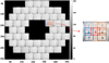 |
Fig. 12 Full field-of-view SHWFS image for the simulated solar granulation on the GLAO and an enlarged sub-aperture image divided into nine GS regions in a 3 × 3 grid. |
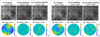 |
Fig. 13 Original focal image under two frames of different aberrations, recovered focal images, the original wavefront, and residual wavefront phase screen for ES-DPRWR and the correlation SHWFS. (a–c) Original focal image with an aberration of RMS=0.563λ, recovered image corrected by ES-DPRWR, and correlation SHWFS, respectively. (d–f) Original wavefront of RMS=0.563λ and residual wavefront for the two methods, respectively. (g–i) Original focal image with an aberration of RMS=0.401λ, recovered image corrected by ES-DPRWR, and correlation SHWFS, respectively. (j–l) Original wavefront of RMS=0.401λ and residual wavefront of the two methods, respectively. |
4.4 Computational latency
We measured the average latency of feature image computation and modal coefficient prediction for ES-DPRWR: 0.038 ms and 0.552 ms, respectively. In this test, latency measurements of 50 000 frames were conducted on one Nvidia GeForce RTX 4080 GPU. The average latency of the computation for one SHWFS feature image using pytorch packages is 10 ms, whereas with cuFFT library it is only 0.038 ms. The CPU clock started before an SHWFS image was imported into the GPU and cut off when all 48 sub-aperture feature images had been computed. The feature images for each sub-aperture were processed in parallel, which significantly accelerated the computational efficiency of this preprocessing. The average latency of modal coefficient prediction without TensorRT acceleration is 4.8 ms, while after TensorRT acceleration it is only 0.552 ms. It is worth noting that the latency of each frame was measured individually. It was just the time of the forward propagation for one SHWFS feature image on the trained network. This way of measurement is in line with the practical AO system operating mode.
Comparison of generalization for the ES-DPRWR network trained on feature images and Riesgo’s network directly trained on solar granulation SHWFS images.
5 Conclusions and discussions
This paper proposes an ES-DPRWR method that is independent of the shape of extended objects. It can achieve high-accuracy measurements of high-spatial-resolution wavefronts on extended scene wavefront sensing. In addition, an ES-DPRWR network trained only once is still capable of achieving a good performance in observing unknown objects.
On the other hand, that great generalizability of ES-DPRWR is because it extracts SHWFS feature images resembling PSFs through a series of frequency-domain processes, which greatly reduces its dependence on the information of observed objects during wavefront measurements. Therefore, the range of the fluctuation magnitude of relative error is only within 6% when the ES-DPRWR trained on the center field of view is tested on other fields of view in the GLAO.
On the other hand, the high measurement accuracy of ES-DPRWR based on SHWFS feature images is because it avoids some limitations caused by slope features on the measurement of high-spatial-frequency aberrations compared to the correlation SHWFS. First, the linear fitting of aberrations in the correlation SHWFS is based on the assumption that the sub-wavefront within each sub-aperture is a plane wave with a certain gradient. Therefore, sub-aperture slope features cannot represent aberrations with spatial frequencies higher than the current spatial sampling rate of the sub-aperture in the SHWFS. This is why the correlation SHWFS can only measure modal aberrations of limited orders. Moreover, the slope feature is a dimension-reduced feature extracted from SHWFS images. It loses a significant amount of detailed information about PSFs – such as their shape, contours, and so on – that is preserved in the feature images. The ES-DPRWR network is even able to extract various unimaginable features from SHWFS feature images by a multitude of convolutional kernels for aberration reconstruction. The excellent nonlinear fitting capability of neural networks enables ES-DPRWR to have a higher accuracy of wavefront estimation compared to the linear fitting of the correlation SHWFS. Thus, it’s not hard to explain why the number of Zernike modal coefficients reconstructed by ES-DPRWR nearly doubles compared with the correlation SHWFS in the experiment, from 35 to 77, and the RMSE of Zernike modal coefficients reconstructed by ES-DPRWR drops by more than one third compared with the correlation SHWFS, from 0.1287 λ to 0.071 λ.
In summary, this manuscript preliminarily demonstrates that ES-DPRWR is capable of achieving a wavefront measurement accuracy superior to that of the correlation SHWFS, and that it also possesses a generalizability far superior to that of the network directly trained on the SHWFS images, although this comes at the cost of a slight loss in accuracy. The computational latency of the ES-DPRWR is roughly sufficient for the daily AO system now, and it can be further optimized in the future.
Certainly, there are additional details regarding ES-DPRWR that are worth further investigation. First and foremost, it would be highly intriguing to delve into the potential applications of ES-DPRWR in a wider range of scenarios, such as not just granulations but larger objects like sunspots or smaller objects completely located within the field of view of the sub-aperture. Based on the theoretical analysis in Sect. 2.2, the ES-DPRWR is theoretically applicable to these scenarios. However, it is noted that different objects may exhibit slightly different forms of noise. Nevertheless, these noises are expected to be resolved by preprocessing. In particular, sunspots or objects completely within the field of view of the sub-aperture tend to have a higher contrast and more distinct spatial details. They may also possess richer high-frequency information in the frequency domain, resulting in potentially less noise in the feature image compared to low-contrast granulations. Consequently, it is plausible to expect that the performance of ES-DPRWR may be superior on high-contrast objects. Experiments to explore the influence of the contrast of the observed extended object on the performance of the ES-DPRWR will be considered in our future work. We will also attempt to use ES-DPRWR to measure wavefronts on the whole GLAO field of view, which will provide more detailed information.
Secondly, there are many contents of ES-DPRWR that deserve optimization. The ES-DPRWR assumes that the object in each sub-aperture is exactly the same. However, for objects that completely fill the field of view of the sub-aperture, there may be different degrees of offset of the object within each sub-aperture due to tilt aberrations or high-order aberrations, which will affect the accuracy of wavefront measurement. The experiments in Sect. 4 have demonstrated that the displacement of sub-aperture objects under the tiltless aberrations at D/r0 = 10 does not have a significant impact on the accuracy of wavefront measurement. In future work, it is necessary for the ES-DPRWR to explore the tolerance range of the offset of the observed object.
Acknowledgements
The authors would like to acknowledge the guide on the use of the GLAO system from Ying Yang, Nanfei Yan, Dingkang Tong, and Xian Ran in the Institute of Optics and Electronics, Chinese Academy of Sciences during experiments. The latency measurements were performed on the real-time controller platform built by Nanfei Yan and the TensorRT enviroment built by Xin Tu. This work was supported by the National Natural Science Foundation of China (12173041, 11727805), Youth Innovation Promotion Association, Chinese Academy of Sciences (No. 2020376), and Frontier Research Fund of Institute of Optics and Electronics, Chinese Academy of Sciences (No. C21K002).
References
- Booth, M. J. 2014, Light Sci. Appl., 3, e165 [NASA ADS] [CrossRef] [Google Scholar]
- Brunner, E., de Visser, C. C., & Verhaegen, M. 2017, JOSA A, 34, 1535 [NASA ADS] [CrossRef] [Google Scholar]
- de Bruijne, B., Vdovin, G., & Soloviev, O. 2022, JOSA A, 39, 621 [NASA ADS] [CrossRef] [Google Scholar]
- Denker, C., Tritschler, A., Rimmele, T. R., et al. 2007, PASP, 119, 170 [NASA ADS] [CrossRef] [Google Scholar]
- DuBose, T. B., Gardner, D. F., & Watnik, A. T. 2020, Opt. Lett., 45, 1699 [NASA ADS] [CrossRef] [Google Scholar]
- Endo, T., Miwa, Y., Ando, T., et al. 2019, in Advanced Maui Optical and Space Surveillance Technologies Conference (AMOS) [Google Scholar]
- Feng, F., Li, C., & Zhang, S. 2018, Opt. Eng., 57, 074106 [NASA ADS] [Google Scholar]
- Guo, Y., Zhang, A., Fan, X., et al. 2016, Opt. Lett., 41, 5712 [NASA ADS] [CrossRef] [Google Scholar]
- Guo, Y., Wu, Y., Li, Y., Rao, X., & Rao, C. 2022a, MNRAS, 510, 4347 [CrossRef] [Google Scholar]
- Guo, Y., Zhong, L., Min, L., et al. 2022b, Opto-Electronic Adv., 5, 200082 [CrossRef] [Google Scholar]
- Kim, D., Choi, H., Brendel, T., et al. 2021, Opto-Electronic Adv., 4, 210040 [CrossRef] [Google Scholar]
- Li, C., Li, B., & Zhang, S. 2014, Appl. Opt., 53, 618 [NASA ADS] [CrossRef] [Google Scholar]
- Nishizaki, Y., Valdivia, M., Horisaki, R., et al. 2019, Opt. Express, 27, 240 [NASA ADS] [CrossRef] [Google Scholar]
- Oberti, S., Correia, C., Fusco, T., Neichel, B., & Guiraud, P. 2022, A & A, 667, A48 [NASA ADS] [CrossRef] [EDP Sciences] [Google Scholar]
- Rao, C., Zhu, L., Rao, X., et al. 2016, ApJ, 833, 210 [NASA ADS] [CrossRef] [Google Scholar]
- Riesgo, F. G., Gómez, S. L. S., Rodríguez, J. D. S., et al. 2022, Opt. Lasers Eng., 158, 107157 [NASA ADS] [CrossRef] [Google Scholar]
- Rouzé, B., Giakoumakis, G., Stolidi, A., et al. 2021, Opt. Express, 29, 5193 [CrossRef] [Google Scholar]
- Schmidt, D., Gorceix, N., Goode, P. R., et al. 2017, A & A, 597, A8 [Google Scholar]
- Smithson, R., & Tarbell, T. 1977, Correlation tracking study for meter-class solar telescope on space shuttle, Tech. rep. [Google Scholar]
- Tyson, R. K., & Frazier, B. W. 2022, Principles of Adaptive Optics (CRC Press) [CrossRef] [Google Scholar]
- Viegers, M., Brunner, E., Soloviev, O., De Visser, C., & Verhaegen, M. 2017, Opt. Express, 25, 11514 [NASA ADS] [CrossRef] [Google Scholar]
- Von Der Lühe, O. 1983, A & A, 119, 85 [Google Scholar]
- Wang, S., Chen, Q., He, C., et al. 2021, A & A, 652, A50 [NASA ADS] [CrossRef] [EDP Sciences] [Google Scholar]
- Wu, Y., Guo, Y., Bao, H., & Rao, C. 2020, Sensors, 20, 4877 [NASA ADS] [CrossRef] [Google Scholar]
- Xin, Q., Ju, G., Zhang, C., & Xu, S. 2019, Opt. Express, 27, 26102 [NASA ADS] [CrossRef] [Google Scholar]
- Yang, Y., Zhang, L., & Rao, C. 2023, MNRAS, 518, 3201 [Google Scholar]
- Zhang, M., & Guo, Y. 2023, IEEE Photonics J., 15, 1 [NASA ADS] [Google Scholar]
- Zhang, C., Wang, S., Zhong, L., Chen, Q., & Rao, C. 2023a, A & A, 674, A126 [NASA ADS] [CrossRef] [EDP Sciences] [Google Scholar]
- Zhang, L., Bao, H., Rao, X., et al. 2023b, Sci. China Phys. Mech. Astron., 66, 269611 [NASA ADS] [CrossRef] [Google Scholar]
- Zhou, Z., Huang, J., Li, X., et al. 2022, PhotoniX, 3, 1 [CrossRef] [Google Scholar]
- Zuo, C., Qian, J., Feng, S., et al. 2022, Light Sci. Appl., 11, 39 [NASA ADS] [CrossRef] [Google Scholar]
All Tables
RMSE of Zernike coefficients for the correlation SHWFS with different numbers of the reconstructed modes.
Comparison of RMSEs (λ) and relative errors of 3rd–299th Zernike coefficients for two methods.
RMSEs and relative errors of modal coefficients reconstructed by ES–DPRWR on nine different GSs.
Comparison of generalization for the ES-DPRWR network trained on feature images and Riesgo’s network directly trained on solar granulation SHWFS images.
All Figures
|
Fig. 1 Negative correlation between both the SR of the focal spot image and the contrast of the focal extended object image, and the magnitude of the single-order modal aberration. Panels a–f show the mapping curves with respect to the 3rd, 20th, 65th, 135th, 230th, and 275th modal aberrations, respectively. For each panel, all the values in the “SR” curve were normalized by dividing by their maximum SR, and similarly all the values in the “Contrast” curve were normalized by dividing by their maximum contrast. |
| In the text | |
|
Fig. 2 Negative correlation between the SR of the focal spot image, the contrast of the focal extended scene image, and the magnitude of the atmospheric turbulence aberration. The value of each point is the average of the contrast of 1000 focal object images under 1000 random aberrations with corresponding D/r0. |
| In the text | |
|
Fig. 3 Computational flow of feature image extraction. |
| In the text | |
|
Fig. 4 Schematic diagram of the ES-DPRWR method. (a) The structure of the ES-DPRWR network. (b) The reconstructed wavefront and the true wavefront. |
| In the text | |
|
Fig. 5 Original solar granulation image and two down-sampled solar granulation images. The size of a sub-aperture image is 20 × 20 in this simulation. Thus, two original solar granulations boxed in red in panel a are down-sampled to panels b and c to satisfy the sub-aperture field of view. |
| In the text | |
|
Fig. 6 Examples of SHWFS images and feature images with the same aberration. Panels d–f show the feature images of corresponding SHWFS images, panels a–c, respectively. In order to compare these three feature images more clearly, the sub-aperture feature images boxed in red in panel d are shown in the first row of panel g, respectively. The second and third rows in panel g show the corresponding sub-aperture feature images in panels e and f, respectively. |
| In the text | |
|
Fig. 7 Two residual images. Panel a shows the residuals of the solar granulation 1 feature image (Fig. 6e) and the point-source feature image (Fig. 6d). Panel b shows the residuals of the solar granulation 1 feature image (Fig. 6f) and the point-source feature image (Fig. 6d). |
| In the text | |
|
Fig. 8 Comparison of residual wavefront phase screens of ES-DPRWR and correlation SHWFS. |
| In the text | |
|
Fig. 9 Performance of the ES-DPRWR network trained on the dataset at D/r0=24 when measuring aberrations at D/r0 of 13–36 for the point source, granulation 1 and granulation 2, respectively. (a) RMSEs. (b) Relative errors. |
| In the text | |
|
Fig. 10 Optical layout of GLAO on the 1-meter NVST (Zhang et al. 2023b). |
| In the text | |
|
Fig. 11 Arrangement of the sub-apertures in the MD-SHWFS. |
| In the text | |
|
Fig. 12 Full field-of-view SHWFS image for the simulated solar granulation on the GLAO and an enlarged sub-aperture image divided into nine GS regions in a 3 × 3 grid. |
| In the text | |
|
Fig. 13 Original focal image under two frames of different aberrations, recovered focal images, the original wavefront, and residual wavefront phase screen for ES-DPRWR and the correlation SHWFS. (a–c) Original focal image with an aberration of RMS=0.563λ, recovered image corrected by ES-DPRWR, and correlation SHWFS, respectively. (d–f) Original wavefront of RMS=0.563λ and residual wavefront for the two methods, respectively. (g–i) Original focal image with an aberration of RMS=0.401λ, recovered image corrected by ES-DPRWR, and correlation SHWFS, respectively. (j–l) Original wavefront of RMS=0.401λ and residual wavefront of the two methods, respectively. |
| In the text | |
Current usage metrics show cumulative count of Article Views (full-text article views including HTML views, PDF and ePub downloads, according to the available data) and Abstracts Views on Vision4Press platform.
Data correspond to usage on the plateform after 2015. The current usage metrics is available 48-96 hours after online publication and is updated daily on week days.
Initial download of the metrics may take a while.