| Issue |
A&A
Volume 637, May 2020
|
|
|---|---|---|
| Article Number | A99 | |
| Number of page(s) | 14 | |
| Section | Astronomical instrumentation | |
| DOI | https://doi.org/10.1051/0004-6361/201935109 | |
| Published online | 28 May 2020 | |
Wide field-of-view, high-resolution Solar observation in combination with ground layer adaptive optics and speckle imaging
1
The Key Laboratory on Adaptive Optics, Chinese Academy of Sciences, PO Box 350, Shuangliu, Chengdu, 610209 Sichuan, PR China
2
The Laboratory on Adaptive Optics, Institute of Optics and Electronics, Chinese Academy of Sciences, PO Box 350, Shuangliu, Chengdu, 610209 Sichuan, PR China
e-mail: This email address is being protected from spambots. You need JavaScript enabled to view it.
3
Southwest Institute of Technical Physics, Chengdu, 610041 Sichuan, PR China
Received:
23
January
2019
Accepted:
12
March
2020
Abstract
Context. High angular resolution images at a wide field of view are required for investigating Solar physics and predicting space weather. Ground-based observations are often subject to adaptive optics (AO) correction and post-facto reconstruction techniques to improve the spatial resolution. The combination of ground layer adaptive optics (GLAO) and speckle imaging is appealing with regard to a simplification of the correction and the high resolution of the reconstruction. The speckle transfer functions (STFs) used in the speckle image reconstruction mainly determine the photometric accuracy of the recovered result. The STF model proposed by Friedrich Wöger and Oskar von der Lühe in the classical AO condition is generic enough to accommodate the GLAO condition if correct inputs are given. Thus, the precisely calculated inputs to the model STF are essential for the final results. The necessary input for the model STF is the correction efficiency which can be calculated simply with the assumption of one layer turbulence. The method for calculating the correction efficiency for the classical AO condition should also be improved to suit the GLAO condition. The generic average height of the turbulence layer used by Friedrich Wöger and Oskar von der Lühe in the classic AO correction may lead to reduced accuracy and should be revised to improve photometric accuracy.
Aims. This study is aimed at obtaining quantitative photometric reconstructed images in the GLAO condition. We propose methods for extracting the appropriate inputs for the STF model.
Methods. In this paper, the telemetry data of the GLAO system was used to extract the correction efficiency and the equivalent height of the turbulence. To analyze the photometric accuracy of the method, the influence resulting from the distribution of the atmospheric turbulence profile and the extension of the guide stars are investigated by simulations. At those simulations, we computed the STF from the wavefront phases and convolved it with the high-resolution numerical simulations of the solar photosphere. We then deconvolved them with the model STF calculated from the correction efficiency and the equivalent height to obtain a reconstructed image. To compute the resulting photometric precision, we compared the intensity of the original image with the reconstructed image. We reconstructed the solar images taken by the GLAO prototype system at the New Vacuum Solar Telescope of the Yunnan Astronomical Observatory using this method and analyzed the results.
Results. These simulations and ensuing analysis demonstrate that high photometric precision can be obtained for speckle amplitude reconstruction using the inputs for the model STF derived from the telemetry data of the GLAO system.
Key words: instrumentation: adaptive optics / instrumentation: high angular resolution / techniques: image processing / techniques: high angular resolution / Sun: general
© L. Zhong et al. 2020
 Open Access article, published by EDP Sciences, under the terms of the Creative Commons Attribution License (http://creativecommons.org/licenses/by/4.0), which permits unrestricted use, distribution, and reproduction in any medium, provided the original work is properly cited.
1. Introduction
Life on the Earth is greatly influenced by the state of the Solar atmosphere. It is important to investigate Solar physics and monitor the active regions on the Solar surface in order to ultimately have the ability to predict space weather based on observations of the Sun. As the Solar atmosphere is highly structured and dynamic, in many cases the observation of the small-scale structure at a wide field of view (FOV) on the Sun is crucial for considering important scientific questions (Rimmele & Marino 2011). Atmospheric turbulence degrades the angular resolution of the images captured by the ground-based optical telescopes. The distribution of the 3D turbulence shows that the distortions in the ground layer account for a large amount of the atmospheric turbulence along the transmitted path. Conjugating and correcting only the ground layer turbulence make the correction effective over a wide FOV. In 2001, Rigaut (Rigaut 2002) proposed the ground layer adaptive optics (GLAO) system in which only one deformable mirror (DM) is used to conjugate with the most intense ground layer turbulence. In GLAO, the multi-direction Shack Hartman wavefront sensor (MD-SHWFS; Langlois et al. 2004; von der Lühe et al. 2005) is used to detect the distortions from multi-field angles and the wavefront phases are averaged to control the shape of the single low order DM. It is capable of offering a relative, homogeneously improved image quality over a very large FOV. The advantages of the increased resolution in a wider FOV make the GLAO an appealing complementary mode for AO which can potentially contribute to a more efficient use of the telescope if both the observational program and the AO mode are chosen wisely (Schmidt et al. 2017).
The GLAO system generally attempts to correct a larger FOV more homogeneously than classical AO and the correction of the GLAO system at the lock patch is most often moderate and not diffraction-limited. The effect of the GLAO correction is equivalent to achieving a visible improvement to some extent, while the residual aberrations of the system still unavoidably degrade the image quality. Thus, post facto image processing techniques are required to further improve the quality of the observations on the whole FOV. GLAO provides a less well-performing but more homogeneous correction across the FOV than classical AO, this makes the combination of GLAO and image reconstruction particularly interesting. The speckle imaging technique (Labeyrie 1970; Weigelt 1977; Zhong et al. 2014) has been demonstrated as one of the suitable methods for reconstructing solar images. In speckle imaging, the object’s Fourier phases and the Fourier amplitudes are estimated from a sequence of randomly distorted short exposure images. The Fourier phases are reconstructed by the bispectrum method (Weigelt 1977; Pehlemann & von der Luehe 1989) or the cross-spectrum method (Knox & Thompson 1974). Then there is the Labeyrie method (Labeyrie 1970), which is used to recover the Fourier amplitudes of the object. By inverse Fourier transformation of the Fourier amplitudes and Fourier phases of the object, the high-resolution image of the object can be obtained.
In the speckle image reconstruction of the AO images, the AO system ensures that the effects of atmospheric seeing surmount the telescope’s aberration, thus supporting even more strongly the assumptions inherent to the derivation of the speckle masking method and as far as the recovery of Fourier phases is concerned, AO correction actually enforces the underlying theory of Fourier phase reconstruction (Denker et al. 2005). As a result, the photometric properties in the reconstructed images are primarily affected by the Fourier amplitude calibration and the Fourier phase reconstruction is not very relevant, so it is not further considered in this paper. In the reconstruction of the Fourier amplitudes, the model speckle transfer function (STF; Wöger & von der Lühe 2007) that is commonly used enables the photometrically successful calibration of AO speckle imaging data. The inputs for the model STF proposed by Friedrich Wöger and Oskar von der Lühe (Wöger & von der Lühe 2007) are the Fried parameter and the correction efficiency of the AO system. Other factors may influence the accuracy of the model STF, including the number of included correction scenarios and telescope elevation angles, etc. A residual photometric error will always remain. A detailed analysis of those influences can be found at the reference (Peck et al. 2017) and it is not further discussed here. The accuracy of those inputs determines the photometric accuracy of the reconstruction. Although the Fried parameter r0 is the most important input for the model STF with regard to the largest impact on the shape of the STF (Peck et al. 2017), it is not further discussed in this paper because there are several methods for determining the Fried parameter and the influence for the final reconstruction is homogeneous. In this paper, the Fried parameter is calculated from a fitting of the variances for the open loop Zernike mode coefficients recovered from the GLAO simultaneously controlling information and the corresponding values predicted by the Kolmogorov turbulence (Rimmele 2010) based on the least squares method. On the contrary, the correction efficiency generally varies and is field-dependent, so we mainly discuss the method used to obtain the correction efficiency by the GLAO system at the directions out of the WFS detected FOV using the simultaneous control information.
For classical AO correction, because of the influences from the anisoplanatism effect of the atmosphere, the correction of the system is field-dependent and near diffraction limit imaging can only be achieved at the boresight of the wavefront sensor. Field-dependent STFs are needed to get photometric reconstruction at a large FOV. To obtain the effective correction efficiencies, the simultaneous wavefront information is needed. Restricted by the limited information about the atmospheric turbulence, the simplified statistical results are employed. The assumption of a single layer of turbulence placed at the estimated height has been proposed by Friedrich Wöger and Oskar von der Lühe (Wöger & von der Lühe 2007). This relieves us from making calculations about the temporally varying turbulence profile  which cannot be given by the AO wavefront sensor. In their procedure, the position is assumed to be equal to the empirical generic average height of the turbulence at the observation site. As the high variability of the seeing conditions during the day require the measurement of the turbulence information to be strictly simultaneous with the observations, it can be inferred that the photometric accuracy of the reconstruction resulting from this simplification is unreliable and the accuracy will be influenced by two factors: (1) the departure between the real generic average height with the empirical one and (2) the accuracy of the simplification using the real generic average height.
The aim of the GLAO system is to partially correct the atmospheric turbulence over a large FOV. After GLAO correction, the residual phase and the correction efficiency will not be statistically the same because the Ground layer phase information is obtained from the average of the wavefront from all guide directions. The correction can provide a visible homogeneously improvement of the quality at the FOV of the MD-SHWFS, but the image quality off the FOV of the MD-SHWFS is decreased for the spatial de-correlation of the turbulence phases and the lack of the phase information at those directions. As has been mentioned previously, the performance of the GLAO system still critically depends on the vertical distribution of the turbulence profile (Peter 2010). Therefore, an important scientific issue is based on evaluating the variation of image quality over the observation FOV (Andersen et al. 2006). In the reconstruction process, this leads to the field-dependent correction efficiency and the variation on the shape of the STF with field angle. From the process of modeling the STFs at the classical AO condition, it is known that this model STF is generic enough to accommodate GLAO system if correct inputs are given. To get model STFs in the GLAO condition, except of the Fried parameter, the field-dependent correction efficiency is also needed. However, unlike the CAO system in which only one guide patch is used to detect the distortions, the GLAO system uses the mean wavefront information calculated from multi field directions to drive the DM, thus the evaluation of the effective correction efficiency at the whole FOV should be considered in a different way. This paper is devoted to proposing a photometrically reliable method to calculate the input parameters for the model STFs in the speckle imaging reconstruction.
In the GLAO system, the wavefront information from multi guide directions can be used to derive a more reliable assumption about the turbulence. In this paper, the equivalent height calculated from real-time MD-SHWFS measurements and the GLAO control information in a best-fitting method is proposed to calculate the effective correction efficiency at the off guide directions. This method derives more reliable correction efficiency as the input for the model STF and enables the photometrically successful calibration of GLAO speckle imaging data. To analyze the photometric accuracy of the method, the influences from the turbulence profile distribution and the patterns of the guide star (GS) were investigated from simulations of both the atmospheric turbulence and the correction of the GLAO system. It can be shown that the photometric accuracy of the reconstruction from the equivalent height is higher than the results calculated from the analytical generic average height at all the simulated cases and the method contributes to a reliable reconstruction with high photometric accuracy across the whole FOV. The images obtained from the GLAO prototype system (Kong et al. 2016, 2017) at the New Vacuum Solar Telescope (NVST) were reconstructed using the method proposed and the results were analyzed.
The paper is organized as follows: in Sect. 2, we briefly describe the speckle image reconstruction of the AO images and the main procedures in the speckle image reconstruction of the GLAO images. Especially, we propose the method, based on the use of the equivalent height of the turbulence to reconstruct the GLAO images. Section 3 describes the details of the simulations to testify to the photometric accuracy of the method. Section 4 presents the results, with the key points in the reconstruction of the GLAO images described in detail and the results evaluated. Section 5 presents the main conclusions of this work.
2. Speckle image reconstruction of the GLAO images
2.1. Speckle image reconstruction of AO images
As the model STF from the Kolmogorov spectrum is not suitable for the post processing of the AO images and the accuracy of the model STF is vital to the photometry of the final reconstruction, the reconstruction of the object’s Fourier amplitude from the AO images must be treated in an unusual way. The procedures proposed by the Friedrich Wöger and Oskar von der Lühe (Wöger & von der Lühe 2007) are commonly used to get the STF after AO correction. This section is devoted to providing an introduction to the method. The details can be found in the reference. The main inputs for the model STF are the Fried parameter and the correction efficiency of the AO system. For the reason described at the introduction, the influences from the Fried parameter are ignored and the calculation of the field depended correction efficiency are analyzed. The correction efficiency of the AO system on the ith Zernike mode βi is defined as:
 (1)
(1)
where  is the variance of the coefficients corresponding to the ith Zernike mode in the residual wavefront errors and the
  is the variance of the coefficients corresponding to ith Zernike mode in the original wavefront errors before the AO correction.
To get the effective correction efficiency at the off guide directions, given the lack of the information about the wavefronts, the statistical results from the turbulence profile are used. The correction efficiency of the ith Zernike mode can be estimated from the correction efficiency at the guide direction and the covariance coefficients of the wavefront phases from the two directions:
 (2)
(2)
Here, 0 is the guide direction of the AO system, the γ is field angle of the off guide direction and coefi(0,γ) is the covariance of the ith Zernike mode coefficients at the field angles 0 and γ, which is defined as:
 (3)
(3)
Theoretically, the spatial covariance coefficients are a function of the Zernike mode number, the separated field angle distance γ, and the  of the turbulence. Given the limited information about the simultaneous turbulence profile in most of the system, the assumption of one single turbulence layer is used to simplify the calculation:
 (4)
(4)
where h̄ is the height of the assumed single-layer turbulence that is given. The single-layer turbulence can be assumed as positioned in the generic average height, which is calculated from the expression bellow (Roddier et al. 1982):
![Mathematical equation: $$ \begin{aligned} \bar{h}^ * = \left[ {\frac{\int _{0}^{H} {h^{5 \mathord {\left. \right. } 3}C_n^2 (h)\mathrm{d}h} }{\int _{0}^{H} {C_n^2 (h)\mathrm{d}h} }} \right]^{3 \mathord {\left. \right. } 5}. \end{aligned} $$](/articles/aa/full_html/2020/05/aa35109-19/aa35109-19-eq9.gif) (5)
(5)
Given the lack of the simultaneous refractive index structure constant, the empirical generic average height of the turbulence at the observation site is used instead (Wöger & von der Lühe 2007). However, besides the reduced accuracy resulting from the difference between the analytical generic average height and the empirical one, the photometric accuracy of the reconstruction using the analytical one has not been analyzed in the reference either. As the generic average height is usually used to calculate the isoplanatic angle of the turbulence, which is the angular distance where the atmospheric turbulence is essentially unchanged, it has no information about the effects when the angular distance is larger than the isoplanatic angle. Thus, it may not suitable for getting the correction coefficients at the off guide directions.
2.2. The speckle image reconstruction of GLAO images
In the GLAO system, the wavefront aberrations Ws(r) which the DM is intended to correct are the mean value of the wavefronts from multi directions detected by the MD-SHWFS:
 (6)
(6)
where M is the number of Zernike mode that the MD-SHWFS can detect, N is the number of guide patch in the system, and ai(γk) is the corresponding coefficient of the ith Zernike mode at the field angle of γk. Due to the errors of the GLAO system, the correction is also never complete. The correction efficiency of the GLAO system is defined as the function of the mean wavefront information calculated from the N guide directions. It represents the correction ability of the GLAO system and not the actual value at any field angle.
As the performance of the GLAO system is not uniform across the whole FOV (Andersen et al. 2006) and the actual correction efficiency by the GLAO at some specific field angles is needed in the speckle image reconstruction process, it is necessary to calculate the field depended effective correction efficiency.
Statistically, the compensated phase by the GLAO system at the ith Zernike mode of the wavefront can be expressed as:
 (7)
(7)
and the total compensated phase by the GLAO system is:
 (8)
(8)
As the GLAO system uses only one DM conjugated at the ground layer, the correction is identical around the whole FOV. The compensated phase at one specific field angle, γ, is equal to the one of the GLAO system, Wc(r). By expressing the phase as the function of the correction efficiency at the field angle γ, we get the equation below:
 (9)
(9)
From the relationship above, the correction efficiency of the ith Zernike mode at the field angle γ can be deduced (see Appendix A) as:
 (10)
(10)
The equation shows that the calculation of the effective correction efficiency at the off guide directions corrected by the GLAO system also requires the covariance coefficients. Due to the defects involved in using the empirical generic average height for calculating the covariance coefficients discussed above, the equivalent height calculated from the telemetry data of GLAO system is proposed to get more reliable results, which is discussed in the following paragraph.
2.3. The equivalent height of the turbulence
To get an equivalent height at the meaning of the covariance coefficients for calculating the correction efficiency of the GLAO system in the speckle image reconstruction process, the covariance coefficients which can be calculated from the telemetry data in the GLAO system are used as the criteria. The covariance relationship between guide directions can be calculated from corresponding open loop wavefront information which were recovered from the recorded residual wavefront errors and the correction data of the GLAO system. When the number of guide field is N, there are  covariance coefficient sequences can be used.
We define ai(γ1) as the ith Zernike mode coefficient of the recovered open loop wavefront at the field angle γ1. There are N sets of original coefficients at field angles γ1, γ2, γ3, …, γN, thus the experimental covariance coefficients can be obtained as:
 (11)
(11)
To find the best-fit equivalent height, the analytical covariance coefficients corresponding to a sequence of tested equivalent height hj are calculated. The j represents the index at the sequence of the tested equivalent height and the corresponding coefficient. The range of the tested equivalent height and the step of the sequence are user defined. The analytical value calculated at the tested equivalent height hj is:
 (12)
(12)
To pick the best-fit equivalent height in the process, the Euclidian distances between the experimental values and the analytical ones are chosen as the criterion:
 (13)
(13)
The equivalent height is considered as H, when the corresponding Euclidian distance d is the minimum value at the sequence. In this case, the covariance coefficient calculated from the equivalent height approximately equal to the experimental value calculated by the wavefront phases from the guide directions at the meaning of the Euclidian distance. As the method considers all the available turbulence information within the FOV of the MD-SHWFS, it may give reliable results at the wide FOV image reconstruction system.
After getting the equivalent height, the effective correction efficiencies at the field angles away from the guide directions can be calculated using the Eqs. (10) and (4). With the effective correction efficiency, the model STFs used in the speckle reconstruction can be obtained.
3. The simulations
Using the method proposed above, we attempt to calculate the spatial decorrelation coefficients of the optical modes based on information about only one turbulence layer. The position of the turbulence layer is assumed to be at the equivalent height which has been estimated from the experimental covariance coefficients calculated from the wavefront information at the guide directions. Thus, the accuracy of the method may depend on the profile of the turbulence and the distribution of the GS. The aim of this part of the paper is to investigate the influence of the atmospheric turbulence profile and GS patterns on the performance of the method. The simulations with anisoplanatic atmosphere and partially corrected GLAO system were applied and the photometric accuracy of the reconstructions were tested. The object for the simulation is one diffraction-limited sub-patch of the solar granulation image which is shown in Fig. 1.
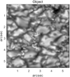 |
Fig. 1. Solar granulation used as the object. |
To simplify the simulations and focus on main factors, the detected errors of the MD-SHWFS are neglected. The correction efficiency of the GLAO system in the simulation is displayed in Fig. 2 which is supposed to be same as the one of our GLAO system at the first 27 Zernike modes. The tip and tilt correction efficiencies are set at 100% for the alignment process of the speckle reconstruction.
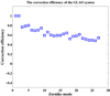 |
Fig. 2. Correction efficiency of the GLAO system. |
The recovered open loop wavefront information from guide directions is used to estimate the equivalent height of the turbulence using Eq. (13). After getting the equivalent height, the correction efficiency at the off guide directions can be obtained to calculate the STFs in the speckle image reconstruction. The results calculated from the generic average heights are also displayed in each condition for comparison. To get rid of the influence from the accuracy of the recovered Fourier phases, the Fourier phases used in the reconstruction are the true Fourier phases derived from the Fourier transform of the object.
To quantitatively illustrate the performance of reconstructions as a function of the GS extension and the turbulence profile distribution, the image distance and the intensity correlation coefficient defined by Mikurda and von der Lühe (Mikurda & von der Lühe 2006) have been carried out. Before the evaluation, the mean values of the reconstructions and the truth image are normalized to 1. The speckle reconstruction are symbolized by  and the truth image is symbolized by I0(X).
The intensity correlation coefficient is defined as the variance of reconstruction divided by the variance of truth image:
 (14)
(14)
The Euclidian image distance of truth and reconstructed images is determined as:
 (15)
(15)
where A is the area of the images. From the definitions, it is obvious that the intensity correlation coefficient approaching 1 and the image distance approaching 0 are the demonstrations for a high photometric accuracy reconstruction.
To give an intuitional representation of the accuracy, the absolute intensity distance between the object and the reconstructions that are calculated from the two heights is displayed in Figs. 6 and 10 in the following two sub-sections. The absolute intensity is defined as  . The range of the label at the right side of the figure is from the minimum value to the maximum value of the absolute intensity distance with four steps.
3.1. The influences from the structure of the turbulence
In this section, the influence of the turbulence profile distribution on the accuracy of the method is considered. The atmospheric turbulence is simulated as a discrete set of thin turbulent layers and the propagation of the wavefront through such layers. The turbulence profile considered in the simulation is the one which is commonly used by researchers, namely, the Hufnagle-Valley (HV) model. The HV model can be generalized into the following form, capable of representing any  profile as the sum of exponential terms (Hardy 2000):
 (16)
(16)
In this expression, A is the coefficient for the surface (boundary layer) turbulence strength and HA is the height of its 1/e decay, B and HB similarly define the turbulence in the troposphere (up to about 10 km), C and HC define the turbulence peak at the tropopause. In order to study the effects of turbulence model on the accuracy of the method, three possible scenarios are considered: the HV 5-7 model, HV 10-10 model, and HV 15-12 model of the turbulence profile. Parameters used in the three typical turbulence models are listed in Table 1. The entire Fried parameters r0 and the isoplanatic angles θ0 specified at wavelength of 0.5 μm for the three turbulence are given in the last two columns.
Constants for turbulence models.
Every model is simulated by the four respective layer phases. The location and the strength of the phase layers are calculated from the method presented by P. Wallner and Richard G. Paxman et al. (Wallner 1994; Paxman et al. 1999). The altitudes and the relative  of those layers for the three models are listed in the Table 2. Each layer contains one big phase. Time evolution in this case is simulated by resorting to the Taylor hypothesis: large phase screen are generated and turbulence is frozen so that time evolution is due to the movement of such layers which is simulated by shifting the phase screens according to their velocities (Femenia et al. 2002). The wind direction for all the layers are the same for simplification. With the effect of the wind flow, 1000 phase screens are obtained at each condition.
Distribution of the turbulence model and the corresponding assumed single layer height.
Due to fact that the typical scenario for a GLAO system is to shoot a symmetric pattern of GS to sky surrounding the imaged area (Korkiakoski et al. 2006), GS are placed in a circle around the corrected field. Figure 3 shows three different patterns commonly used by the researchers. The stars in those patterns represent the GSs and the points are the test field angles. For the symmetric pattern of the GS extension, only the results from the first quarter of the field are displayed. Pattern I has one GS at the field origin and four GSs evenly at the circle around the field, which is the same as the one used in our GLAO system described in the next part of the paper. Pattern II only has four GSs around the field and Pattern III has half of the stars moved inside the field and half of the stars outside. In this part, the GS extension is chosen as pattern I. The other guide patterns are used in the sub-section to analyze the influence from the distribution of the GS on the photometric accuracy of the reconstruction.
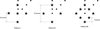 |
Fig. 3. Distribution of the GS (stars) and the tested field angles (points) at the three patterns. |
The generic average height and the equivalent height at each model are shown in Table 2. The generic average heights at the three turbulence profile are calculated from Eq. (5). The equivalent height is calculated from the wavefront information at the guide directions. To investigate the accuracy of the covariance coefficients calculated from those single-layer assumptions, Eq. (17) defines the distance between the actual covariance coefficients and the covariance coefficients calculated from the generic average height or the equivalent height. The angular distance is spread from 0″ to 32″ with step 2″, with the results shown in Fig. 4. The turbulence profile is the HV 5-7 model and the isoplanatic angle of this turbulence profile is 1.4″. We have:
 (17)
(17)
where coefi(γ,0) is the actual covariance coefficients of the ith Zernike mode when the angular distance is γ,  is the estimated covariance coefficient obtained when the h̄ is set to be the generic average height or the equivalent height. M is the number of the Zernike mode used and is set to be 27 in the calculation below.
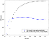 |
Fig. 4. Distance between the actual covariance coefficient and the estimated covariance coefficient calculated from the equivalent height and the generic average height with the angular distance as the variable. |
From the figure above, it is obvious that the equivalent height can give acceptable results at all the tested field angular distances and the generic average height is only suitable for the calculation of the covariance coefficient when the field angular distance is around the isoplanatic angle and show a large departure from the actual one as the angular distance become larger. This phenomenon coincides with the analysis described above.
In the segmentation process of the speckle image reconstruction, to get rid of the anisoplanatic effect, the whole image is divided into sub-images with each FOV approaching the isoplanatic angle. To calculate the correction efficiency at a specific field angle, the covariance coefficient calculated from the angular distance between the specific sub-direction and the guide directions are needed. Those angular distances are mainly larger than the isoplanatic angle, so the accuracy of the covariance coefficients with larger angular distance are more important for the high photometric accuracy reconstruction. The evaluations of the reconstruction shown below further demonstrate the validity of this method.
In the speckle image reconstruction, a full diffraction-limited reconstruction with photometric accuracy is required and only a high performance STF can deliver this. To testify to the performance of the two heights on the reconstruction, the correction efficiency, the corresponding STFs, and the absolute distance of the image intensity are calculated. The results for the HV 5-7 model are shown in Figs. 5 and 6.
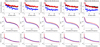 |
Fig. 5. Results obtained from the simulations (in black), the generic average height (in blue), and the equivalent height (in red) at the tested field angles when the turbulence profile follows the HV 5-7 model. Rows, from top to bottom: effective correction efficiency, modal STF, and power spetrum of the reconstruction. |
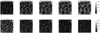 |
Fig. 6. Absolute distance between the reconstructions and the object at the tested field angles. The results at the top row are calculated from the generic average height and the results at the bottom row are calculated from equivalent height. The turbulence profile follows the HV 5-7 model. A common scale for those images that correspond to the same used height is used and the scales for different heights are different. The scales of the images corresponding to the same height are placed at the right side of the images. |
At the guide directions and the directions out of the detected FOV, the experimental correction efficiencies calculated from the wavefront phase information and the analytical values when the single-layer turbulence is placed at the equivalent height and generic average height are shown in the first row of Fig. 5. Simulated values (in black) are calculated from the standard deviation of the residual phases,  , and the standard deviation of the original phases,
  , at given field angle, γ, using Eq. (1), which facilitate the direct computation of the experimental values of the system and therefore set the “ground truth” for a test of the analytical values. The analytical values are both calculated from Eq. (2). Where the covariance coefficients in Eq. (2) are calculated from Eq. (4) using the generic average height (in blue) or the equivalent height (in red), individually.
The lack of information about the turbulence which is spread along the whole transmitted path, leads to a departure of the simulated results from the analytical values calculated from the single layer model. The corresponding STFs calculated from those correction efficiencies are given in the second row of Fig. 5. The power spectrum of the reconstruction are shown at the last row of the figure. The abscissa is normalized to the theoretical spatial cut-off. The colors of those lines are similarly defined as the correction efficiency condition. Although the accuracy of the analytical values are slightly different among those field-angle distances due to the variant accuracies of covariance coefficients, the equivalent height gives better fitting results than the generic average height in all those tested field angles and shows a striking similarity to the “ground truth”.
The absolute intensity distances between the reconstructed image and the object intensity are shown in Fig. 6, which gives a direct measurement of the photometric accuracy of the method. The mean values of those images are normalized to 1 for easy comparison. The results demonstrate that the equivalent height calculated from the proposed method gives more reliable results for this turbulence profile model.
Figure 7 shows the evaluation of the three turbulence models at all the tested field angles. The intensity correlation coefficient indicates to what extent the variance of the object is recovered. The recovered intensity correlation coefficient approach to 1 in all the equivalent height cases and spread from 1.5 to 2.7 at the generic average height cases. The results of the image distance coincide with the conditions of the intensity correlation coefficient. The increase of the intensity correlation coefficient and the image distance between the reconstruction from the generic average height and the truth image can be explained by the underestimate of the correction efficiency and the relative STF which amplify the high frequency part of the recovered power spectrum. It is immediately seen that the reconstruction from the equivalent height are more closer to the object than the results from generic average height at all the three turbulence profiles.
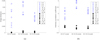 |
Fig. 7. Image distance and correlation coefficient of the truth image and the reconstructed intensity from the generic average height (blue) and the equivalent height (black) at different field angles with the change of the turbulence profile. |
The simulations above give the results as the distribution of the turbulence layer, following the classical turbulence profile which contains significant turbulence layer within the first 200m above the ground. This is the foundation of the GLAO system. As the turbulence departure from the classical turbulence profile and the strength of the turbulence concentrates on two or more turbulence layers, the analysis about the accuracy of the equivalent height on the reconstruction is important for the universality of this method. Table 3 below shows the parameters for the three artificial turbulence profiles. These turbulence profiles are based on the classical HV 5-7 model, but the relative  weighting of each layer is reset to obtain non-classical turbulence profiles. The accuracy of the reconstructions using the equivalent height at those conditions have also been evaluated on the basis of the image distance and the intensity correlation coefficient. The results are shown at the Fig. 8.
Distributions of the artificial turbulence profiles and the corresponding assumed single layer heights.
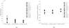 |
Fig. 8. Image distance and correlation coefficient of the truth image and the reconstructions from the equivalent height at different field angles with the change of the turbulence profile. |
The results show that the accuracy of the reconstruction using the equivalent height slightly depend on the distribution of the turbulence profile. Taking the cases of classical HV 5-7 model, the artificial model I, and the artificial model II into consideration: in the classical model, the turbulence mainly concentrates on one layer and the accuracy of the reconstruction are high. As the strength of the turbulence spreads to two or more layers, the accuracy of the reconstruction slightly decreases due to the error from the equivalence of the turbulence with the single-layer phase. After analyzing the photometric accuracy of the reconstruction of the condition of the artificial model II and the artificial model III, it is shown that the position of the equivalent height has little effect on the accuracy of the reconstruction.
The simulations above demonstrate that the equivalent height can deliver reliable reconstructions even when the turbulence profiles are non-classical and concentrate on two or more turbulence layers. This is because that the equivalent height gives a generalized value considering all the available information.
3.2. The influences from the pattern of the GS
The major advantages that solar AO systems have over night-time systems are: it has an infinite amount of lock structures available (due to the extended nature of the Sun). That means that virtually any reasonable guide pattern is possible, as long as the wavefront sensor configuration supports it. However, for the comprehensive performance of the wavefront sensor, the distribution of the GS are usually chosen to be the several classical patterns. The distribution of the GS and the field angles which the evaluation taken place are shown in Fig. 3. This part is devoted to analyzing the influences from the distributions of the GS on the accuracy of the method. To simplify the simulation, only the classical HV 5-7 turbulence profile is used at this section. Quantitatively things may change a bit, but not qualitatively.
As in the situation above, the correction efficiencies, the STFs, the power spectrums of the reconstructions, and the absolute image distances at five directions out of the detected FOV in the pattern III condition are shown in Figs. 9 and 10. The meanings of the symbols and colors are similarly defined as above. As shown, in all the three GS patterns, the correction efficiencies, the related STFs, and the power spectrums give better fitting accuracy at the equivalent height cases than the generate average height cases. The reconstructions from the equivalent height are closer to the real object.
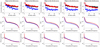 |
Fig. 9. Results obtained from the simulations (in black), the generic average height (in blue), and the equivalent height (in red) at the tested field angles when the turbulence profile follows the HV 5-7 model and the GS distribution is the pattern III. Rows, from top to bottom: effective correction efficiency, modal STF, and power spectrum of the reconstruction. |
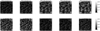 |
Fig. 10. Absolute distance between the reconstructions and the object at the tested field angles. The results at the top row are calculated from the generic average height and the results at the bottom row are calculated from equivalent height. The turbulence profile follows the HV 5-7 model and the GS distribution is the pattern III in the simulations. A common scale for those images that correspond to the same used height is used and the scales for different heights are different. The scales of the images corresponding to the same height are placed at the right side of the images. |
The intensity correlation coefficient and the image distance of the reconstructions from equivalent height and generic average height at all the three GS patterns are shown in Fig. 11. For the symmetry distribution of all the tested field angles, the evaluations at the same field angular distance away from the central field are only displayed once. It can be seen in these figures that the results from the equivalent height give a better accuracy. Thus, the single layer model which the turbulence placed at the equivalent height can deliver an excellent result. Also, the GS distribution has a negligible effect on equivalent height performance. Because the calculation of the generic average height still needs information on the turbulence profile, the benefit of the fitting method over using a more generic average height is the simplification and the effectiveness it offers.
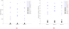 |
Fig. 11. Image distance, correlation coefficient of the truth image, and reconstructed intensity from the generic average height (blue) and the equivalent height (black) at different field angles with the change of the GS pattern. |
From the simulation and analyses above, it is obvious that the photometric accuracy of this method across the whole FOV is hardly influenced by the turbulence condition and the distribution of the GS. As the method gives high accuracy results at all the simulated conditions, it is reasonable to infer that the method can deliver reliable results for most of the observation situations.
4. Experiment results
4.1. The GLAO prototype system
The TiO band images acquired from he GLAO prototype system mounted at the NVST are reconstructed by the method proposed above. The prototype system uses the MD-SHWFS to detect the wavefront phases. The frame rate of the MD-SHWFS camera is 800 Hz and the sub-aperture array at the MD-SHWFS is arranged hexagonally. Although there are 7 × 7 sub-apertures configured, only 30 effective sub-apertures are used in the wavefront sensing due to the secondary obscuration of the telescope. The arrangement of the sub-apertures and the five guide sub-fields in each sub-aperture are displayed in Fig. 12. The FOV of each sub-aperture is about 60″ × 52″ with the pixel scale at 0.5″/pixel. The separated field angle between the adjacent guide fields in the horizontal and vertical direction is 16″. And the FOV of the sub-field is 12″ × 10″ (Kong et al. 2016, 2017). Thus, the separated field angles between those five guide fields are one of three types: 16″, 22.6″, 32″. Incidentally, the MD-SHWFS image in Fig. 12 is not acquired simultaneously with the GLAO image shown in Fig. 13, but the alignment relationship between this TiO band image and the simultaneous MD-SHWFS image can be used to co-align those two types of images until the imaging system is changed.
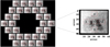 |
Fig. 12. Arrangement of the available sub-apertures in the MD-SHWFS and one of the corresponding sub-apertures with the guide field number marked. |
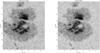 |
Fig. 13. Open loop image (left) and GLAO image with the five guide patches marked (right). These are arbitrary images which were not acquired simultaneously. |
The GLAO prototype system saw its first experiment on January 12th, 2016. The active region NOAA 12599 was observed by the system around the time [UT] 5:35:55, October 7th, 2016. The GLAO image and the corresponding open loop image obtained are shown at Fig. 13. A noticeable improvement of the image quality without reaching the diffraction limit over the whole FOV is typical for the low order GLAO correction. To co-align the MD-SHWFS image with the far field GLAO image, we rotate the wavefront image with 134° and shift the GLAO image at TiO band by [102,43] pixels. The five guide fields in the MD-SHWFS projected onto the TiO band image are shown on the right side of Fig. 13.
Estimating the imaging quality of extended object after the correction of GLAO system is not carried out directly as in the stellar case. To quantitatively illustrate the GLAO performance from the images, the generalized Fried parameter (Berkefeld et al. 2005; Schmidt et al. 2017) is usually used. The generalized Fried parameter is an estimation of the Fried parameter (Fried 1966) when the correction is applied. The distributions of generalized Fried parameters across the whole FOV calculated from the open loop image sequence and the GLAO image sequence are given in Fig. 14. Without GLAO, the mean value of those generalized Fried parameters is about 11 cm at TiO band (705.7 nm) and the image quality is uniform across the whole FOV. With GLAO correction, the mean value of those generalized Fried parameters increases to 14.9 cm. And from the distribution of the generalized Fried parameter, it can be seen that the effective correction FOV is about 30″ which relates to the detection FOV of the MD-SHWFS. Out of the effective correction FOV, the image quality is also improved but less. Due to the improvement of the resolution by the GLAO is limited and field depended, the speckle imaging technique with field depended STFs is needed for further improving the quality of the whole FOV image.
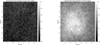 |
Fig. 14. Distribution of the generalized Fried parameter for each isoplanatic patch encoded as a gray scale map across the whole FOV calculated from the open loop image sequence (left) and the GLAO image sequence (right). |
4.2. Estimation of the parameters of the turbulence
To obtain the Fried parameter and the equivalent height of the turbulence which are needed for calculating the STF in the speckle image reconstruction, the wavefront information of the full turbulence measurements are required. In the GLAO prototype system, the real time information of the DM drive signals and the residual wavefront errors at five guide directions are recorded during the operation. Those data are used to reconstruct the information on the open loop atmospheric turbulence. This is achieved by adding the DM’s voltages projected onto the wavefront distortions and the residual wavefront errors calculated from the slopes recorded in the observation (Cortes et al. 2012).
The wavefront information in the five guide-field directions are used to calculate the Fried parameters and the correction efficiency. The Fried parameters are calculated from fitting the variances of the Zernike mode coefficients and the corresponding values predicted by the atmospheric Kolmogorov variance (Rimmele 2010). In this procedure, the mean value of the Fried parameters calculated from all the guide directions is considered as the actual Fried parameter of the turbulence and used to reconstruct the GLAO image in the speckle imaging technique.
The equivalent height of the turbulence are calculated from Eq. (13). When the tested equivalent height values distributed from 2000 m to 4000 m with 80 steps, the best fitted equivalent height is 3164.6 m. The results shown in Figs. 15a–d illustrate the experimental values and the best-fit analytical values when the separated field angles are 16″, 22.6″, 32″, respectively.
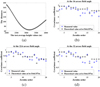 |
Fig. 15. Panel a: sum of the Euclidian distance between the experimental covariance coefficients and the analytical values calculated from Eq. (13) with different equivalent height values. The equivalent height values are distributed from 2000 m to 4000 m with 80 steps and the best fitted equivalent height is 3164.6 m. Panels b–d: experimental values and best-fit analytical values when the separated field angle are 16″, 22.6″, 32″, respectively. |
From Fig. 15, it is can be seen that analytical values and the observations reveal deviations at some Zernike modes. The main reason contributes for the deviations is the assumption of the 3D distributed turbulence with a single-layer phase screen placed at the equivalent height in the best-fit method which is discussed earlier in this paper. As we know, there are other three factors that may influence the precision of the model. On one hand, the accuracy of the MD-SHWFS measurement is related to the number of sub-apertures in the MD-SHWFS and characteristics of the object in the guide patch. On the other hand, the central obscuration of the telescope has an effect on the atmospheric covariances computed by Noll (Noll 1976), which were calculated for an unobstructed entrance pupil. In the last, the number and the distribution of the guide fields also slightly influence the accuracy of the model. However, the fact is that our method attempts to find the best-fit value between the observation and the model. This contributes the agility and robustness of the process. The method can ensure a relatively stable and acceptable result even when the detection accuracy of the wavefront distortions is low in some circumstances.
After aligning the MD-SHWFS image of the GLAO system with the far field image and getting the equivalent height and Fried parameter of the turbulence, the effective correction efficiency at all the segmented sub-field angles in the speckle reconstruction can be calculated.
The whole reconstruction procedure is summarized below:
-
Obtain the field angles of the guide directions used in the system and estimate the Fried parameter, the equivalent height of the turbulence, and the correction efficiency of the GLAO system on each measurable Zernike mode.
-
Shift and rotate the MD-SHWFS image to align with the GLAO image. Thus, the field angles of the segmented sub-patches at the far-field images can be corresponded to the field angles of the MD-SHWFS image.
-
For every segmented sub-patch in the reconstruction, calculate the effective correction efficiency from the field angle of the sub-patch, the correction efficiency of the GLAO system, and the covariance coefficients.
-
Calculate the STF from the Fried parameter and the effective correction efficiency in each segmented sub-patch, then reconstruct the sub-patch using the speckle imaging technique.
-
Combine the reconstructed patches to get the entire FOV image of the object.
Figure 16 shows the GLAO image and the corresponding speckle reconstruction. The left image in this figure is the optimal example in the image sequence used in the speckle image reconstruction. The median filter-gradient similarity (MFGS) metric proposed by Deng (Deng et al. 2015) is used to assess the quality of the image. In the reconstruction, the size of the segmented patch is 128 × 128 pixels. As the pixel scale is 0.0345″ per pixel, thus, the field angle of the segmented patch is 4.416″ which is within the isoplanatic angle of the turbulence. The Fourier phases are recovered by the bispectrum method. The model STFs corresponding to each segmented patch are numerically evaluated by the Monte Carlo integration algorithms (Wöger & von der Lühe 2007). Visibly, the reconstruction gives higher quality at the whole FOV. To qualify the reconstruction, the residual mean square (RMS) contrast of the image calculated as the standard derivation divided by the mean is used as a relative and quantitative indicator for the image quality. However, it is not a very sensitive measure for the sunspot because the contrast of the sunspot image is dominated by the low-frequency content of the structure. Thus, the RMS contrast of the granulation structure is evaluated. For the sub-images shown in Fig. 17, the mean contrast increase from 2.76% at the GLAO image to 7.46% at the reconstructed image.
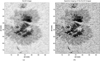 |
Fig. 16. Panel a: original GLAO image, panel b: reconstructed GLAO images. |
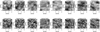 |
Fig. 17. Top row: original GLAO sub-images in the places marked by squares in Fig. 16 and corresponding RMS contrast. Bottom row: corresponding reconstructed sub-images and RMS contrast. |
The contrast of the reconstructed image is slightly low. The discussion below gives some explanation for this result. According to the research of Ricort (Ricort et al. 1981, 1982), the contrast of the observed granulation is influenced by the diameter of the telescope and the observing wavelength, the Fried parameter, and the spatial resolution of the sampling instrument (CCD). The telescope diameter of our system is 0.98 m, the observing wavelength is TiO band (705 nm), and the spatial resolution is 0.0345 arcsec pixel−1. Eliminating the influence from the turbulence, the analytical contrast of the granulation is 13.34%. Except for those factors, the heliocentric angle of the active region observed also influences the contrast of the granulation (Wilken et al. 1997). The active region observed by our system is the NOAA 12599, the position is S15E17, which is not at the disk center; this will further decrease the contrast.
For the reconstructed image, there are also several factors that may influence the contrast of the granulation. One important source for the deviation in contrast could be stray light. This is an important issue and can lead to significant biases in the contrast. The other significant factor is the overestimation of the Fried parameter. The research by Peck has found that the Fried parameter is the most important factor in photometric precision as this parameter appears to have the largest impact on the shape of the STF. The contrast of the reconstruction also depends on the chosen of the Fried parameter. For an underestimated Fried parameter, an insufficient correction to the object’s Fourier amplitudes may be applied and the contrast may increase. On the contrary, for an overestimated Fried parameter, the contrast may decrease. By applying a STF corresponds to a smaller Fried parameter, the contrast of the granulation at the reconstructed image increases from 9.3% to 13.1% (Denker et al. 2005).
The contrast also may be influenced by the unconsidered static aberrations on the STF, etc. Because there are many factors that determine the final contrast of the images and the influence on the contrast is independent of the field angle, we ignore the quantitative value of the contrast and, instead, we pay attention to the fluctuation of the contrast with the field angle. It shows a significant and homogeneous increase of the contrast from Fig. 17, which demonstrates a reliable calculation of the correction ability from our method, albeit indirectly.
5. Conclusion
The GLAO system combined the speckle image technique is attractive for the wide FOV and high resolution observation of the Sun. In the process, the reconstruction of the Fourier amplitude needs the field-dependent model STF proposed by Friedrich Wöger and Oskar von der Lühe. One important input for the STF model is the correction efficiency. In this paper, the accuracy of the calculation for the correction efficiency is improved by using an equivalent height of the atmospheric turbulence. The recovered open loop wavefront information from the close loop data is used to derive the equivalent height. To test the photometric accuracy of the method, the simulations of various turbulence profiles, and different GS patterns are introduced. The results are analyzed by the image distance and the intensity correlation coefficient. The reconstructions using the equivalent height show a greater similarity with the real object than the generic average height. It appears that the method is success for various turbulence profiles and shows weak dependence on the GS patterns. Both of these make the method particularly attractive for use with solar telescopes employing GLAO systems in order to achieve photometrically precise reconstructed images using the Wöger & von der Lühe model. The equivalent height found in this work may also the used as a conjugated height at multi-conjugate adaptive optics (MCAO) system in future. The TiO band images obtained by a GLAO prototype system equipped at the NVST and the corresponding speckle reconstruction are presented. The contrasts of the granulation are improved remarkably and homogeneously. We also demonstrates a reliable calculation of the correction efficiency from our method, indirectly. In conclusion, the method for deriving the correction efficiency as input to the model STF enables the photometrically successful calibration of the GLAO speckle imaging data. In particular, the GLAO correction with speckle image reconstruction suggests its usefulness in future instrumentation projects as a potential observation schema.
Acknowledgments
We appreciate the helpful recommendations from the referees, which enrich the context of this paper and make it more complete. This work is supported by National Natural Science Foundation of China (NSFC) number 11703029, 11727805 and Laboratory Innovation Foundation of the Chinese Academy of Sciences number YJ16K006.
References
- Andersen, D. R., Stoesz, J., Morris, S., et al. 2006, PASP, 118, 1574 [NASA ADS] [CrossRef] [Google Scholar]
- Berkefeld, T., Soltau, D., & von der Luehe, O. 2005, Proc. SPIE, 5903, 219 [NASA ADS] [Google Scholar]
- Cortes, A., Neichel, B., Guesalaga, A., et al. 2012, Proc. SPIE, 8447, 84475T [CrossRef] [Google Scholar]
- Deng, H., Zhang, D., Wang, T., et al. 2015, Sol. Phys., 290, 1479 [NASA ADS] [CrossRef] [Google Scholar]
- Denker, C., Mascarinas, D., Xu, Y., et al. 2005, Sol. Phys., 227, 217 [NASA ADS] [CrossRef] [Google Scholar]
- Femenia, B., Carbillet, M., Riccardi, A., Esposito, S., & Brusa, G. 2002, Proc. SPIE, 4494, 132 [NASA ADS] [CrossRef] [Google Scholar]
- Fried, D. L. 1966, J. Opt. Soc. Am., 56, 1372 [NASA ADS] [CrossRef] [Google Scholar]
- Hardy, J. W. 2000, Phys. Today, 53, 69 [CrossRef] [Google Scholar]
- Knox, K. T., & Thompson, B. J. 1974, AJ, 193, L45 [Google Scholar]
- Kong, L., Zhang, L., Zhu, L., et al. 2016, Chin. Opt. Lett., 14, 6 [NASA ADS] [Google Scholar]
- Kong, L., Zhu, L., Zhang, L., Bao, H., & Rao, C. 2017, IEEE Photonics J., 9, 2662326 [NASA ADS] [Google Scholar]
- Korkiakoski, V. A., Le Louarn, M., & Vérinaud, C. 2006, Proc. SPIE, 6272, 62725A [CrossRef] [Google Scholar]
- Labeyrie, A. 1970, A&A, 6, 85 [Google Scholar]
- Langlois, M., Moretto, G., Richards, K., Hegwer, S., & Rimmele, T. R. 2004, Proc. SPIE, 5490, 59 [NASA ADS] [CrossRef] [Google Scholar]
- Mikurda, K., & von der Lühe, O. 2006, Sol. Phys., 235, 31 [NASA ADS] [CrossRef] [Google Scholar]
- Noll, R. J. 1976, J. Opt. Soc. Am. (1917–1983), 66, 207 [NASA ADS] [CrossRef] [Google Scholar]
- Paxman, R. G., Thelen, B. J., & Miller, J. J. 1999, Proc. SPIE, 3763, 2 [NASA ADS] [CrossRef] [Google Scholar]
- Peck, C. L., Wöger, F., & Marino, J. 2017, A&A, 607, A83 [NASA ADS] [CrossRef] [EDP Sciences] [Google Scholar]
- Pehlemann, E., & von der Luehe, O. 1989, A&A, 216, 337 [NASA ADS] [Google Scholar]
- Peter, D. 2010, Proc. SPIE, 7736, , 77364R [NASA ADS] [CrossRef] [Google Scholar]
- Ricort, G., Aime, C., Roddier, C., & Borgnino, J. 1981, Sol. Phys., 69, 223 [NASA ADS] [CrossRef] [Google Scholar]
- Ricort, G., Borgnino, J., & Aime, C. 1982, Sol. Phys., 75, 377 [NASA ADS] [CrossRef] [Google Scholar]
- Rigaut, F. 2002, European Southern Observatory Conference and Workshop Proceedings, 422 [Google Scholar]
- Rimmele, J. M. T. 2010, Appl. Opt., 49, G95 [CrossRef] [Google Scholar]
- Rimmele, T. R., & Marino, J. 2011, Liv. Rev. Sol. Phys., 8, 2 [Google Scholar]
- Roddier, F., Gilli, J. M., & Vernin, J. 1982, J. Opt., 13, 63 [NASA ADS] [CrossRef] [Google Scholar]
- Schmidt, D., Gorceix, N., Goode, P. R., Marino, J., & von der Lühe, O. 2017, A&A, 597, L8 [NASA ADS] [CrossRef] [EDP Sciences] [Google Scholar]
- von der Lühe, O., Berkefeld, T., & Soltau, D. 2005, C.R. Phys., 6, 1139 [NASA ADS] [CrossRef] [Google Scholar]
- Wallner, E. P. 1994, Proc. SPIE, 2201, 110 [NASA ADS] [CrossRef] [Google Scholar]
- Weigelt, G. P. 1977, Opt. Commun., 21, 55 [NASA ADS] [CrossRef] [Google Scholar]
- Wilken, V., Boer, C. R. D., Denker, C., & Kneer, F. 1997, A&A, 325, 819 [NASA ADS] [Google Scholar]
- Wöger, F., & von der Lühe, O. 2007, Appl. Opt., 46, 8015 [NASA ADS] [CrossRef] [PubMed] [Google Scholar]
- Zhong, L., Tian, Y., & Rao, C. 2014, Opt. Express, 22, 29249 [NASA ADS] [CrossRef] [Google Scholar]
Appendix A: Correction efficiency
In this appendix, the detail calculation leads to Eq. (10) is presented. To obtain the correction efficiency at the Zernike order j in the filed angle γ, we start with Eq. (9). For a specific Zernike order j, a multiplication with aj(γ)Zj(r) on both side of the Eq. (9), we obtain the equation below:
 (A.1)
(A.1)
Taking integration over the pupil and considering the orthogonality of the Zernike polynomials, we can get the equation with a dependency of only the “jth” Zernike order:
 (A.2)
(A.2)
 (A.3)
(A.3)
Because the correction efficiency is statistical value, to make the βj(γ) computable using the information of the turbulence profile, we take the collective average at both sides and finally get Eq. (10) in the main text:
 (A.4)
(A.4)
 (A.5)
(A.5)
All Tables
Distribution of the turbulence model and the corresponding assumed single layer height.
Distributions of the artificial turbulence profiles and the corresponding assumed single layer heights.
All Figures
|
Fig. 1. Solar granulation used as the object. |
| In the text | |
|
Fig. 2. Correction efficiency of the GLAO system. |
| In the text | |
|
Fig. 3. Distribution of the GS (stars) and the tested field angles (points) at the three patterns. |
| In the text | |
|
Fig. 4. Distance between the actual covariance coefficient and the estimated covariance coefficient calculated from the equivalent height and the generic average height with the angular distance as the variable. |
| In the text | |
|
Fig. 5. Results obtained from the simulations (in black), the generic average height (in blue), and the equivalent height (in red) at the tested field angles when the turbulence profile follows the HV 5-7 model. Rows, from top to bottom: effective correction efficiency, modal STF, and power spetrum of the reconstruction. |
| In the text | |
|
Fig. 6. Absolute distance between the reconstructions and the object at the tested field angles. The results at the top row are calculated from the generic average height and the results at the bottom row are calculated from equivalent height. The turbulence profile follows the HV 5-7 model. A common scale for those images that correspond to the same used height is used and the scales for different heights are different. The scales of the images corresponding to the same height are placed at the right side of the images. |
| In the text | |
|
Fig. 7. Image distance and correlation coefficient of the truth image and the reconstructed intensity from the generic average height (blue) and the equivalent height (black) at different field angles with the change of the turbulence profile. |
| In the text | |
|
Fig. 8. Image distance and correlation coefficient of the truth image and the reconstructions from the equivalent height at different field angles with the change of the turbulence profile. |
| In the text | |
|
Fig. 9. Results obtained from the simulations (in black), the generic average height (in blue), and the equivalent height (in red) at the tested field angles when the turbulence profile follows the HV 5-7 model and the GS distribution is the pattern III. Rows, from top to bottom: effective correction efficiency, modal STF, and power spectrum of the reconstruction. |
| In the text | |
|
Fig. 10. Absolute distance between the reconstructions and the object at the tested field angles. The results at the top row are calculated from the generic average height and the results at the bottom row are calculated from equivalent height. The turbulence profile follows the HV 5-7 model and the GS distribution is the pattern III in the simulations. A common scale for those images that correspond to the same used height is used and the scales for different heights are different. The scales of the images corresponding to the same height are placed at the right side of the images. |
| In the text | |
|
Fig. 11. Image distance, correlation coefficient of the truth image, and reconstructed intensity from the generic average height (blue) and the equivalent height (black) at different field angles with the change of the GS pattern. |
| In the text | |
|
Fig. 12. Arrangement of the available sub-apertures in the MD-SHWFS and one of the corresponding sub-apertures with the guide field number marked. |
| In the text | |
|
Fig. 13. Open loop image (left) and GLAO image with the five guide patches marked (right). These are arbitrary images which were not acquired simultaneously. |
| In the text | |
|
Fig. 14. Distribution of the generalized Fried parameter for each isoplanatic patch encoded as a gray scale map across the whole FOV calculated from the open loop image sequence (left) and the GLAO image sequence (right). |
| In the text | |
|
Fig. 15. Panel a: sum of the Euclidian distance between the experimental covariance coefficients and the analytical values calculated from Eq. (13) with different equivalent height values. The equivalent height values are distributed from 2000 m to 4000 m with 80 steps and the best fitted equivalent height is 3164.6 m. Panels b–d: experimental values and best-fit analytical values when the separated field angle are 16″, 22.6″, 32″, respectively. |
| In the text | |
|
Fig. 16. Panel a: original GLAO image, panel b: reconstructed GLAO images. |
| In the text | |
|
Fig. 17. Top row: original GLAO sub-images in the places marked by squares in Fig. 16 and corresponding RMS contrast. Bottom row: corresponding reconstructed sub-images and RMS contrast. |
| In the text | |
Current usage metrics show cumulative count of Article Views (full-text article views including HTML views, PDF and ePub downloads, according to the available data) and Abstracts Views on Vision4Press platform.
Data correspond to usage on the plateform after 2015. The current usage metrics is available 48-96 hours after online publication and is updated daily on week days.
Initial download of the metrics may take a while.