| Issue |
A&A
Volume 687, July 2024
|
|
|---|---|---|
| Article Number | A182 | |
| Number of page(s) | 12 | |
| Section | Astronomical instrumentation | |
| DOI | https://doi.org/10.1051/0004-6361/202449788 | |
| Published online | 12 July 2024 | |
Deep tomography for the three-dimensional atmospheric turbulence wavefront aberration
1
National Laboratory on Adaptive Optics,
Chengdu
610209,
PR
China
e-mail: zhonglibo@ioe.ac.cn
2
Institute of Optics and Electronics, Chinese Academy of Sciences,
Chengdu, Sichuan
610209,
PR
China
3
University of Chinese Academy of Sciences,
Beijing
100049,
PR
China
4
School of Electronic, Electrical and Communication Engineering, University of Chinese Academy of Sciences,
Beijing
100049,
PR
China
Received:
29
February
2024
Accepted:
29
April
2024
Context. Multiconjugate adaptive optics (MCAO) can overcome atmospheric anisoplanatism to achieve high-resolution imaging with a large field of view (FOV). Atmospheric tomography is the key technology for MCAO. The commonly used modal tomography approach reconstructs the three-dimensional atmospheric turbulence wavefront aberration based on the wavefront sensor (WFS) detection information from multiple guide star (GS) directions. However, the atmospheric tomography problem is severely ill-posed. The incomplete GS coverage in the FOV coupled with the WFS detection error significantly affects the reconstruction accuracy of the three-dimensional atmospheric turbulence wavefront aberration, leading to a nonuniform aberration detection precision over the whole FOV.
Aims. We propose an efficient approach for achieving accurate atmospheric tomography to overcome the limitations of the traditional modal tomography approach.
Methods. We employed a deep-learning-based approach to the tomographic reconstruction of the three-dimensional atmospheric turbulence wavefront aberration. We propose an atmospheric tomography residual network (AT-ResNet) that is specifically designed for this task, which can directly generate wavefronts of multiple turbulence layers based on the Shack-Hartmann (SH) WFS detection images from multiple GS directions. The AT-ResNet was trained under different turbulence intensity conditions to improve its generalization ability. We verified the performance of the proposed approach under different conditions and compared it with the traditional modal tomography approach.
Results. The well-trained AT-ResNet demonstrates a superior performance compared to the traditional modal tomography approach under different atmospheric turbulence intensities, various turbulence layer distributions, higher-order turbulence aberrations, detection noise, and reduced GSs conditions. The proposed approach effectively addresses the limitations of the modal tomography approach, leading to a notable improvement in the accuracy of atmospheric tomography. It achieves a highly uniform and high-precision wavefront reconstruction over the whole FOV. This study holds great significance for the development and application of the MCAO technology.
Key words: turbulence / atmospheric effects / instrumentation: adaptive optics / telescopes
© The Authors 2024
 Open Access article, published by EDP Sciences, under the terms of the Creative Commons Attribution License (https://creativecommons.org/licenses/by/4.0), which permits unrestricted use, distribution, and reproduction in any medium, provided the original work is properly cited.
This article is published in open access under the Subscribe to Open model. Subscribe to A&A to support open access publication.
1 Introduction
The observation of ground-based telescopes is seriously disturbed by atmospheric turbulence. The use of adaptive optics (AO) can overcome this limitation (Jiang 2018). However, the performance of traditional AO systems is limited by atmospheric anisoplanatism (Fried 1982), resulting in a limited correct field of view (FOV) of typically just a few arcseconds, which cannot meet the demand for an observation with a large FOV. Multiconjugate adaptive optics (MCAO) can overcome the above limitations. It was first proposed by Beckers (1988) and has been proved in night-time and solar observations (Marchetti et al. 2007; Rao et al. 2018). MCAO uses multiple wavefront sensors (WFSs) to simultaneously detect the wavefront from multiple guide star (GS) directions, and atmospheric tomography techniques are employed to obtain the wavefront aberrations caused by atmospheric turbulence at different altitudes by using the detected wavefronts from multiple GS directions. After the three-dimensional atmospheric turbulence wavefront aberration distribution is obtained, multiple deformable mirrors conjugated to turbulence layers at different altitudes are employed to perform a layered correction of atmospheric turbulence. This ultimately achieves a three-dimensional aberration correction over a large FOV. Figure 1 shows a schematic of the three-dimensional wavefront aberration detection.
Modal tomography is currently the research focus in atmospheric tomography technology, which was proposed by Ragazzoni et al. (1999). The wavefront of each turbulence layer and the wavefront of each GS direction are spatially related in projection. When the heights of multiple turbulence layers and the positions of multiple GSs are determined, the projection matrix is also determined. The traditional approach of modal tomography can be regarded as solving the L = AW problem, where L represents the wavefront of multiple turbulence layers, A denotes the projection matrix, and W represents the wavefront detected by the WFS from multiple GS directions. The conventional solution to this problem is the least-squares (LS) approach. However, since the tomographic reconstruction of the three-dimensional atmospheric turbulence wavefront is an ill-posed inverse problem (Ellerbroek & Vogel 2009; Ramlau & Rosensteiner 2012; Stadler & Ramlau 2022), the projection matrix contains low singular values, and even a small detection error can seriously affect the final solution of the three-dimensional wavefront, resulting in a limited accuracy of the three-dimensional wavefront aberration reconstruction using this method. Despite the application of truncated singular value decomposition (TSVD) to constrain the singular values of the projection matrix, the LS method still exhibits a limited aberration reconstruction accuracy over the whole FOV (Fusco et al. 2001a). Fusco et al. (1999, 2001a,b) optimized the problem using maximum a posteriori (MAP) approach, adding prior information on atmospheric turbulence aberrations and detection noise to the reconstruction matrix. Compared with the conventional LS approach, the reconstruction accuracy of three-dimensional wavefront aberrations was significantly improved, but the performance in the GS uncovered area is still not satisfactory. On the basis of incorporating atmospheric turbulence aberration prior information, He (2016) introduced the Tikhonov regularization method for optimizing the reconstruction matrix. This method obtained a high Strehl ratio (SR) in the GS coverage area, but the SR in the GS uncovered area is still not satisfactory. Some iterative solvers have also been proposed to solve the ill-posed problem, such as the Fourier domain iterative solver (Yang et al. 2006; Vogel & Yang 2006), the Kaczmarz iterative solver (Ramlau & Rosensteiner 2012; Rosensteiner & Ramlau 2013), the FEWHA iterative solver (Stadler & Ramlau 2022; Yudytskiy et al. 2014; Yudytskiy 2014), and the gradient-based iterative solver (Ramlau & Saxenhuber 2016). These methods iteratively solve the problem while incorporating prior information, which alleviates the ill-posed problems to a certain extent, thereby enhancing the reconstruction accuracy of three-dimensional wavefront aberrations and reducing the computational complexity involved in problem-solving. However, these methods still perform poorly in the GS uncovered area, and the problem of nonuniform accuracy in the whole FOV aberration reconstruction still persists. Although compared to traditional AO technology, the MCAO technology has greatly improved the aberration detection accuracy over a large FOV, the limited accuracy of existing tomographic reconstruction algorithms for the atmospheric tomography ill-posed problem restricts the advantages of the MCAO technology to some extent; it has not yet fully realized its advantages. Therefore, the problem of achieving a high precision three-dimensional wavefront aberration tomographic reconstruction over the whole FOV and of further improving the high-resolution imaging observation of the MCAO technology in large FOV still needs to be solved.
Machine-learning has made significant progress in recent years (Jordan & Mitchell 2015). The artificial neural network (ANN) and the convolutional neural network (CNN), which are composed of neural networks, are representative algorithms of machine-learning, and they have been widely used in the field of AO (Guo et al. 2022) due to their high fitting ability, high real-time performance, and high generalization ability. For example, CNNs can directly recover the wavefront aberration from far-field intensity images (Nishizaki et al. 2019; Guo et al. 2019; Orban de Xivry et al. 2021). Compared to traditional phase-retrieval algorithms (Gerchberg & Saxton 1972; Gonsalves 1982), this approach has improved the wavefront reconstruction speed significantly. CNNs enable a direct wavefront reconstruction based on Shack-Hartmann (SH) WFS images (Hu et al. 2019, 2020; Guo et al. 2021), eliminating the centroid and slope calculation process. Moreover, this approach yields a notable improvement in the wavefront reconstruction accuracy. Osborn et al. (2014) proposed a ANN-based multi-object adaptive optics (MOAO) system (Osborn et al. 2014), which can output on-axis WFS slopes from multiple input off-axis WFS slopes. The ANN model was trained on experimental datasets and achieved good results in on-sky implementation, proving that the neural network-based algorithm can be used for atmospheric tomography and that the model trained on experimental datasets can be used for practical observations.
Deep-learning is one of the most representative algorithms in machine-learning (LeCun et al. 2015). It is a data-driven algorithm that uses deep neural networks composed of multiple neural network layers to learn the mapping relation between input and output data from large datasets. Similarly, it can also learn the spatial projection relation between wavefronts of multiple lines of sight and the wavefront of multiple turbulence layers. The impact of this ill-posed problem on the precision of a three-dimensional wavefront reconstruction has to be addressed. To solve the problem of the nonuniform wavefront reconstruction accuracy over the whole FOV using traditional modal tomography, we used a deep-learning-based method to perform the tomographic reconstruction of the three-dimensional atmospheric turbulence wavefront aberration. We propose an end-to-end approach and an atmospheric tomography residual network (AT-ResNet) structure to address this atmospheric tomography problem. This approach simplifies the SH WFS centroid calculation, SH WFS slope calculation, wavefront reconstruction, and aberration tomography steps in the modal tomography approach by employing AT-ResNet to directly output the Zernike coefficients of multiple turbulence layers based on the SH WFS images from multiple GS directions. It significantly improves the accuracy of the large FOV wavefront aberration detection, thereby overcoming the limitations of traditional modal tomography. This approach holds significant importance for high-resolution imaging observations with a large FOV in the MCAO system.
We only considered open-loop conditions. We assumed that all measurements and corrections are performed instantaneously, thereby neglecting the temporal aspects of MCAO operations. Hence, we focused on the spatial aspects of atmospheric tomography and correction, enabling us to provide explicit interpretations of the results. However, this approach is not limited to open-loop conditions. It can also be applied to closed-loop conditions and will also demonstrate superior results compared to the traditional modal tomography approach in the closed-loop case.
The structure of this paper is as follows: in Sect. 2, the simulation modeling method of multiple turbulence layers and multiple GSs, the deep-learning-based approach, and the traditional modal tomography approach are introduced. In Sect. 3, the deep-learning-based approach and the traditional modal tomography approach are compared under different atmospheric turbulence conditions, various turbulence layer distributions, a higher-order turbulence aberration condition, an SH WFS detection noise condition, and a reduced GSs condition. Finally, a summary of the entire study and an outlook on future research are provided in Sect. 4.
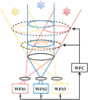 |
Fig. 1 Schematic diagram of the three-dimensional wavefront aberration detection. |
Atmospheric subdivision results.
2 Method
2.1 Simulation modeling method
To reconstruct the three-dimensional atmospheric turbulence wavefront aberration, it is necessary to perform atmospheric subdivision as an initial step. In this study, the atmospheric subdivision was conducted based on the principles outlined in Wallner (1994),
![$\[\left\{\begin{array}{l}\int_{h_m}^{H_m} C_n^2(h)\left(h-h_m\right)^{\frac{2}{3}} \mathrm{~d} h=\int_{H_{m-1}}^{h_m} C_n^2(h)\left(h_m-h\right)^{\frac{2}{3}} \mathrm{~d} h \\H_m=\frac{h_m+h_{m+1}}{2},\end{array}\right.\]$](/articles/aa/full_html/2024/07/aa49788-24/aa49788-24-eq1.png) (1)
(1)
where Hm, Hm−1, and hm correspond to the upper and lower boundaries and to the position of the turbulence layer, respectively. C2n(h) represents the turbulence profile, and we used the HV5/7 model (Hufnagel 1974),
![$\[\begin{aligned}C_n^2(h)= & 3.59 \times 10^{-53} h^{10} \mathrm{e}^{-\left(\frac{h}{1000}\right)}+2.7 \times 10^{-16} \mathrm{e}^{-\left(\frac{h}{1500}\right)} \\& +1.7 \times 10^{-14} \mathrm{e}^{-\left(\frac{h}{100}\right)}.\end{aligned}\]$](/articles/aa/full_html/2024/07/aa49788-24/aa49788-24-eq2.png) (2)
(2)
The equivalent atmospheric coherence length r0m of each turbulence layer can be obtained from Eq. (3),
![$\[r_{0 m}=\left[0.423 k^2 \int_{H_{m-1}}^{H_m} C_n^2(h) \mathrm{d} h\right]^{-\frac{3}{3}},\]$](/articles/aa/full_html/2024/07/aa49788-24/aa49788-24-eq3.png) (3)
(3)
where k = 2π/λ is the wave number, and λ is wavelength.
The upper limit of the atmospheric turbulence height was set as Hmax = 15 km, and the atmosphere was divided into three layers, as shown in Table 1. Most of the turbulence is concentrated in the ground turbulence layer, which is consistent with the actual situation. The datasets we used was generated under various r0 conditions, the telescope aperture was D = 4 m, and the r0m in the table was selected under r0 = 11.43 cm (D/r0 = 35) for presentation.
The wavefront within any circular region can be represented by Zernike polynomials. In the simulation, we used natural GS and the SH WFS for the wavefront detection, because SH WFS cannot detect the piston and the tip-tilt is individually closed-looped by the tracking system. Therefore, each turbulence layer was represented by three ~Jth Zernike coefficients to exclude piston and tip-tilt. The simulation of multiple turbulence layers and multiple GSs was conducted based on the atmospheric subdivision results. Each turbulence layer was equivalent to a phase screen. Figure 2 shows the schematic of the GS detection. The FOV α = 2′, the diameter of each phase screen, can be obtained by Dm = D + 2 × hm × tan(α/2), randomly generated three ~65th Zernike coefficients that conform to the Kolmogorov distribution, which were used to fit each phase screen,
![$\[\Phi_m(R)=\sum_{j=3}^J b_j Z_j(R),\]$](/articles/aa/full_html/2024/07/aa49788-24/aa49788-24-eq4.png) (4)
(4)
where Φm is the wavefront of the m phase screen, J = 65 is the maximum Zernike mode, bj is the coefficient of each Zernike mode, and Zj is each Zernike mode.
Three DMs conjugated to the three turbulence layers were simulated, and each DM can correct three ~65th Zernike coefficients.
The incoming wavefront in each GS direction is given by
![$\[\varphi_n(r)=\sum_{m=1}^M \Phi_m(R)=\sum_{m=1}^M \Phi_m\left(r+\Delta r_{n, m}\right),\]$](/articles/aa/full_html/2024/07/aa49788-24/aa49788-24-eq5.png) (5)
(5)
where ψn is the wavefront of the n GS direction, M = 3 is the phase screen number, and Δrn,m is the position vector between the footprint center of n GS on the m phase screen and the center of the m phase screen.
Six GSs are arranged uniformly at the edge of the FOV, as shown in Fig. 3.
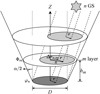 |
Fig. 2 Schematic diagram of the GS detection in multiple turbulence layers. |
 |
Fig. 3 Footprints of six GSs in three turbulence layers. |
2.2 Datasets
The modal tomography approach mainly employs the spatial relation between the incoming wavefronts in multiple GS directions and the wavefronts of multiple turbulence layers to perform the three-dimensional wavefront tomographic reconstruction. Neural networks can learn this spatial relation from large datasets, and the large datasets can also mitigate the ill-posed problems caused by the incomplete spatial detection.
According to the simulation parameters in Sect. 2.1, six SH WFSs were used to detect the incoming wavefronts in multiple GS directions, with a limited detection mode of the first 65 Zernike coefficients. The simulated SH WFS image size was 360 × 360 pixels and had 96 subapertures, each with a circular pupil, and the diffraction-limited spot pattern of each subaperture was mainly sampled by a 3 × 3 pixels array. We normalized the SH WFS image in the range of 0 to 1. This process transforms the data into a consistent scale, which can accelerate the network convergence speed and enhance its performance. Each set of data consisted of the SH WFS images of six GS directions and the Zernike coefficients of multiple phase screens, as shown in Fig. 4. We generated the datasets under the atmospheric conditions of D/r0 = 20 ~ 35 (including mixed data under the conditions of D/r0 = 20, 21, 23...35), 5000 sets of data were generated under each atmospheric turbulence condition, and the final datasets contained 80 000 sets of data. The datasets were divided into training sets, validation sets, and testing sets by 90%, 5%, and 5%. To further test the network performance under different conditions, some additional data were generated, which are introduced below.
2.3 AT-ResNet architecture
As shown in Fig. 5a, the AT-ResNet is proposed to construct the mapping relation between SH WFS images from six GS directions and Zernike coefficients of three turbulence layers. To enhance the nonlinear fitting capability and spatial information extraction ability of the neural networks, we introduced the Funnel ReLU (FReLU) function (Ma et al. 2020) into the network architecture. FReLU uses the max (⋅) nonlinear operation to take the maximum of x and a value, but unlike the ReLU function (Nair & Hinton 2010), FReLU extends it to two-dimensional, addressing the issue that the ReLU function is insensitive to spatial information and enabling a more effective image feature extraction. Figure 5b shows its schematic diagram. The expression of FReLU is shown in Eq. (6),
![$\[\begin{aligned}& f\left(x_{c, i, j}\right)=\max \left(x_{c, i, j}, T\left(x_{c, i, j}\right)\right) \\& T\left(x_{c, i, j}\right)=x_{c, i, j}^w \cdot p_c^w\end{aligned}\]$](/articles/aa/full_html/2024/07/aa49788-24/aa49788-24-eq6.png) (6)
(6)
where f(⋅) is the FReLU nonlinear activation function, xc,i,j is the input pixel in the cth channel, T(⋅) is the funnel condition, xwc,i,j is a kh × kw size parametric pooling window centered on xc,i,j, pwc is the learnable coefficient on this window, which is shared in the same channel, and (⋅) is the point multiplication.
AT-ResNet has seven ResBlocks, which is an improved version based on the bottleneck in He et al. (2016); its structure is shown in Fig. 5d. ResBlock replaces the ReLU function with FReLU on the basis of the bottleneck to improve the spatial feature extraction ability. Additionally, it introduces coordinate attention (Hou et al. 2021), as shown in Fig. 5c, to improve the feature extraction capacity, enabling a better learning of crucial features in multidirection SH WFS images. ResBlock can address the degradation problem in deep-learning (He et al. 2016), thereby enabling the network to learn more hierarchical features and improving the performance of network. We used overlap maximum pooling (Maxpooling) to down-sample the feature map. This can extract the main features and remove redundant information, and it reduces the risk of overfitting to a certain extent. The batch normalization (BN) layer ensures a consistent data distribution (Ioffe & Szegedy 2015), while it also avoids gradient disappearance and gradient explosion, and it accelerates the convergence speed.
Table 2 shows the detailed parameter configuration of AT-ResNet. SH WFS images from six GS directions were fed into network. The network input size was 6 × 360 × 360. Then the image features were extracted by convolutional layers, Max-pooling layers, and bottleneck layers. After passing through the global average pooling layer, the feature map size was converted into 2048 × 1 × 1. The global average pooling operation calculates the average value of the feature map and directly gives each channel a significance value to represent the corresponding feature map. Furthermore, it reduces the model parameters and computational complexity, effectively mitigating the overfitting risk. The last fully connected layer output size was 1 × 189, and after concatenation, the data dimension was transformed to 3 × 63, representing the three ~65th Zernike coefficients of the three wavefront phase screens.
2.4 Training
The network training parameters in this paper are consistent with the following settings. The network was trained on the D/r0 = 20 ~ 35 datasets. We set the batch size to 12, the initial learning rate to 0.0006, and the learning rate decays by 0.85 times every ten epochs. Adam is a gradient-based stochastic optimization algorithm (Kingma & Ba 2014). We took Adam as the optimization algorithm in the training process. The root mean square error (RMSE) was used as the loss function,
![$\[\operatorname{RMSE}(y_{i, j}, \hat{y}_{i, j})=\sqrt{\frac{\sum_{i=1}^{\operatorname{Num}}(y_{i, j}-\hat{y}_{i, j})^2}{\text { Num }}},\]$](/articles/aa/full_html/2024/07/aa49788-24/aa49788-24-eq7.png) (7)
(7)
where yi,j is the estimated jth Zernike coefficient of the i phase screen, ![$\[\hat{y}_{i, j}\]$](/articles/aa/full_html/2024/07/aa49788-24/aa49788-24-eq23.png) is the truth jth Zernike coefficient of the i phase screen, and Num is the total number of Zernike modes of the three phase screens.
is the truth jth Zernike coefficient of the i phase screen, and Num is the total number of Zernike modes of the three phase screens.
During the training process, the loss was computed between the estimated Zernike coefficients and the truth Zernike coefficients. The gradients of the loss of the network weights were then calculated using the back-propagation loss, and the network weights were updated through the ADAM optimizer. This process aims to minimize the difference between the network output and the standard output, gradually approaching the standard output. The AT-ResNet was trained on NVIDIA GeForce RTX 3090 GPU for 100 epochs. The training process took about 180h.
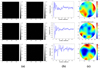 |
Fig. 4 Panel a: standard input: SH WFS images of six GS directions. Panels b and c: standard output: three-layer phase screen wavefront. |
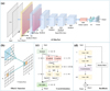 |
Fig. 5 Structure of (a) AT-ResNet. The schematic diagram of (b) the FReLU function, (c) the CoordAttention, and (d) ResBlock. |
Detailed parameter configuration of the SF-ResNet architecture.
2.5 Traditional modal tomography approach
The coming wavefronts in multiple GS directions and the wavefronts of multiple turbulence layers are spatially related,
![$\[L=A W,\]$](/articles/aa/full_html/2024/07/aa49788-24/aa49788-24-eq24.png) (8)
(8)
where L = [L1 L2 . . . LN]T is the wavefront matrix of N GS directions, W = [W1 W2 . . . WM]T is the wavefront matrix of M turbulence layers, and A is the projection matrix, which is only related to the height of multiple turbulence layers and the position of multiple GSs.
The traditional modal tomography approach mainly uses the detected wavefronts from multiple WFSs and the projection matrix A to solve the L = AW inverse problem to obtain W. However, the incomplete GS coverage in the FOV will cause large condition numbers in matrix A, which significantly impacts the solution of multiple turbulence layers. We employed the generalized Tikhonov regularization method to optimize the solution of L = AW, as shown in Eq. (9), which is an improved version of He (2016). This method was used as a comparison to the deep-learning-based method,
![$\[W=\left(A^{\mathrm{T}} A+\varepsilon K\right)^{+} A^{\mathrm{T}} L \text {, }\]$](/articles/aa/full_html/2024/07/aa49788-24/aa49788-24-eq25.png) (9)
(9)
where the plus represents the generalized inverse. ε is the regularization coefficient obtained using the generalized cross-validation (GCV) method (Golub et al. 1979), which avoids ill-posed solutions caused by low singular values, enabling a better solution of Eq. (9). The matrix K is the turbulence covariance prior matrix that imposes constraints on the solution, which can be calculated from Noll (1976).
3 Results and discussion
3.1 Results from the testing sets
The well-trained AT-ResNet was tested on 4000 sets of D/r0= 20 ~ 35 testing sets. Figure 6 shows the average results of AT-ResNet on the entire test set, where the SR of various lines of sight is the average SR of 50 uniformly selected points in that line of sight. The average SR of AT-ResNet in various lines of sight is above 0.9. The performance degradation is not significant in the regions with a low GS coverage at the edge of the FOV, and it still maintains a high precision. The whole FOV SR map shows that the aberration reconstruction accuracy of AT-ResNet will only degrade to a certain extent at the edge of the FOV, but the lowest SR in the whole FOV is also above 0.85, and the average SR of the whole FOV is 0.97, achieving highly uniform and high precision results in the three-dimensional wavefront aberration tomographic reconstruction over the whole FOV.
In addition, we randomly selected a set of data to test AT-ResNet and compare it with the traditional modal tomography (MT) approach. Figures 7 and 8 show the comparison results of the two methods on this testing set. With increasing altitude, the GS coverage in the FOV decreases, leading to an increased difficulty in the reconstruction of turbulence layers at higher altitudes. However, the results demonstrate that AT-ResNet can effectively reconstruct multiple turbulence layers with very little reconstruction error. In addition, the reconstruction accuracy of the higher-altitude turbulence layers does not degrade significantly, and AT-ResNet still achieves a high accuracy in the reconstruction of higher-altitude turbulence layers. Although the higher-altitude turbulence layers have small original aberrations, the incomplete GS coverage seriously affects the reconstruction accuracy of the MT approach. It exhibits substantial reconstruction residuals in higher-altitude turbulence layers, and it only has high reconstruction accuracy in the ground turbulence layer. The MT approach performs less well in the reconstruction of multiple turbulence layers than AT-ResNet. Figure 8 shows that MT exhibits a noticeable degradation in the aberration reconstruction in regions with a lower GS coverage. The average SR of AT-ResNet in this testing set is 0.97, which is better than the 0.77 of MT. These results demonstrate the significant advantage of AT-ResNet.
We calculated the computation time of the two approaches. The computation time of AT-ResNet was tested on a NVIDIA GeForce RTX 3090 GPU and accelerated using NVIDIA TensorRT8.6 INT8 mode. The computation time of MT was tested on an Intel i9-11900K CPU. The results are shown in Table 3. The MT approach involves an extensive matrix computation, and the determination of the regularization coefficient ε also requires significant computation, resulting in a long computation time of 35.2134 ms. Despite the long training time of the AT-ResNet, the computation time of the well-trained AT-ResNet is fast. The computational time of AT-ResNet after acceleration with TensorRT is only 3.0299 ms, which is significantly better than the 35.2134 ms of MT. Although the computational speed of AT-ResNet currently does not meet the real-time control requirement of the MCAO system, it does not represent the ultimate limit of the computation speed of AT-ResNet. Its computational speed can be further accelerated by leveraging advanced hardware devices, performing neural network pruning, and employing other acceleration approaches to fulfill the real-time control demand.
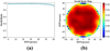 |
Fig. 6 Average results of AT-ResNet for all testing sets. Panel a: SR curves of various lines of sight. Panel b: whole FOV SR map. |
3.2 Performance under different turbulence intensity conditions
We generated 2000 sets of data each under D/r0 = 10, 15, 20... 50 conditions to test the two methods under different turbulence intensity conditions. Because of the incomplete GS coverage in the whole FOV, especially in the center and at the edge of the highest turbulence layer, this seriously affects the atmospheric tomography accuracy of the traditional MT approach. As shown in Fig. 9, the accuracy of AT-ResNet is significantly higher than that of the MT approach, regardless of whether under weak or strong turbulence conditions. As D/r0 increases from 20 to 35, the performance degradation of AT-ResNet is not obvious. The average SR of the whole FOV decreases from 0.99 to 0.96, which is a decrease of only 0.03. In contrast, the MT approach exhibits a more significant degradation: The average SR decreases from 0.83 to 0.70, which is a reduction of 0.13 and prevents us from achieving a high-precision three-dimensional wavefront aberration reconstruction under strong turbulence conditions. The advantage of AT-ResNet is particularly evident in the regions with low GS coverage at the edge of the FOV. In the case of strong turbulence with D/r0 = 35, the SR of the MT approach at the edge of the FOV is only about 0.4. The limited aberration detection accuracy imposes constraints on the advantages of MCAO technology. In contrast, the SR at the edge of the FOV of the AT-ResNet still remains at about 0.9, and AT-ResNet achieves a high-precision aberration reconstruction over the whole FOV.
We tested the two methods under different turbulence intensity conditions. As shown in Figs. 10a and b, AT-ResNet achieves a high SR in various lines of sight under D/r0 = 10~50 conditions, and the SR generally remains above 0.8. It only exhibits a significant performance degradation under D/r0 = 50 strong turbulence condition. In contrast, as the turbulence intensity increases, the MT exhibits a remarkable performance degradation, which is particularly evident for D/r0 = 50. The highest SR is only about 0.7, and the SR at the edge of the FOV drops to about 0.3. AT-ResNet is trained on datasets in the range of D/r0 = 20~35, as shown in the blue area in Fig. 10c. Remarkably, even without specific training for untrained conditions, AT-ResNet also performs very well. The average SR of the whole FOV is above 0.8 for D/r0 = 10~50, which is significantly better than the MT. Consistent with the above results, this advantage is more evident under strong turbulence conditions. These results indicate that AT-ResNet is capable of learning the spatial projection relation between the incoming wavefronts in multiple GS directions and the wavefronts of multiple turbulence layers from extensive datasets. The well-trained AT-ResNet is also applicable to the untrained turbulence intensity data. It is worth noting that the performance of AT-ResNet clearly degrades for D/r0 = 50, but this can be compensated for by expanding the range of the training turbulence intensity and by increasing the number of datasets.
Computation time of the two approaches.
3.3 Effect of the reduced GSs
In an MCAO system, multiple SH WFSs are used to detect the incoming wavefronts in multiple GS directions. Reducing the GS number for wavefront sensing can effectively reduce the complexity and cost of the MCAO system. However, this reduction in GS number also results in a decreased GS coverage in the FOV. As a result, this introduces challenges in solving the ill-posed problem and increases the difficulty of the three-dimensional wavefront aberration reconstruction. We decreased the GS number from six to three, as shown in Fig. 11, and investigated the impact of the reduced GSs on the two approaches.
Only in this section did AT-ResNet use datasets from three GSs, and it was retrained under three GSs conditions. The training datasets are consistent with those in Sect. 2.2, but only the three GSs data shown in Fig. 11 were used as input. The AT-ResNet input size was 6 × 360 × 360. The two methods were compared on 2000 sets of D/r0 = 35 data for three and six GSs. The results are shown in Figs. 12a–c. Under the reduced GSs condition, both approaches exhibit a decrease in the detection accuracy of the whole FOV aberration. The SR map reveals a noticeable performance degradation of AT-ResNet in regions without GS coverage, while it still maintains high SR in regions with GS coverage. Comparing the results under six GSs, the whole FOV average SR decreased from 0.96 to 0.87. In contrast, MT exhibits a significant performance degradation, with the highest SR in the SR map reaching only around 0.4. The whole FOV average SR decreases from 0.7 under six GSs to 0.33, indicating a substantial decline compared to the performance of AT-ResNet. Figure 12c shows that MT achieves an SR of only approximately 0.2 at the edge of the FOV under three GSs. Moreover, AT-ResNet performs far better under three GSs than MT under six GSs.
Figure 12d shows the whole FOV average SR on D/r0 = 10~50 testing sets. The performance degradation of MT under three GSs is remarkably evident, with both a low whole FOV average SR and a large standard deviation. This indicates the highly unstable three-dimensional wavefront aberration reconstruction capability of MT under three GSs, making it challenging to effectively solve the ill-posed problem. Although AT-ResNet shows a certain performance degradation under strong turbulence conditions with three GSs, the degraded performance is also acceptable. Moreover, the AT-ResNet with three GSs consistently outperforms the MT with six guide stars under different turbulence intensities. These results demonstrate that AT-ResNet can effectively overcome the impact of reduced GSs, which is of great significance in practical applications.
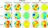 |
Fig. 7 Reconstruction results of three-layer phase screens for one testing set using AT-ResNet and MT. |
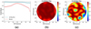 |
Fig. 8 (a) Comparison of SR curves between the two methods from one testing set. The whole FOV SR map of (b) AT-ResNet and (c) MT from one testing set. |
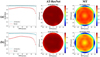 |
Fig. 9 Comparison of AT-ResNet and MT for (a) D/r0 = 20 and (b) D/r0 = 35 conditions. |
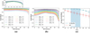 |
Fig. 10 SR curves of various lines of sight of (a) AT-ResNet and (b) MT under different turbulence intensity conditions. (c) Comparison of the whole FOV average SR between AT-ResNet and MT under different turbulence intensity conditions. |
 |
Fig. 11 Footprints of three GSs in three turbulence layers. |
3.4 Robustness to variations in the turbulence layer distribution
In practical observations, the height measurement of multiple turbulence layers may be biased, and there may be additional turbulence layers between the measured turbulence layers. Since the turbulence layer distribution in the datasets used to train the neural network was fixed, the wavefronts of multiple turbulence layers output by the network were also mapped to the fixed training heights. The network learns the mapping relation from the detection information in multiple GS directions to the wavefronts of multiple fixed-height turbulence layers. Therefore, when the actual turbulence layer distribution differs from the turbulence layer distribution in the datasets, the actual mapping relation between the detection information in multiple GS directions and the wavefronts of the multiple turbulence layers also undergoes changes, thereby affecting the three-dimensional wavefront aberration reconstruction accuracy of the network and further affecting the whole FOV aberration correction effect.
In this section, the robustness of the approach to the turbulence layer height offset and additional turbulence layers was tested. First, for the condition D/r0 = 35, keeping the height of the ground turbulence layer unchanged, the heights of the second and third turbulence layers were offset within the range from – 20% to 20%. For each case, 2000 sets of data were generated for the testing. The well-trained parameters of AT-ResNet and the reconstruction matrix of the MT remained unchanged. The wavefronts of multiple turbulence layers output by AT-ResNet and MT were still mapped to the heights set in Sect. 2.2. We compared the robustness of the two approaches to the turbulence layer height offset. The test results are shown in Fig. 13. Compared to the case without a height offset, when there is a height offset to the turbulence layers, AT-ResNet shows a decrease in various lines of sight of the SR and in the whole FOV average SR. However, within the range of −10% to 10% of the height offset, its performance degradation is not significant, and it still maintains a high SR performance. Only when the height offset reaches −20% does the performance degradation become more obvious. The MT approach demonstrates a higher stability against the turbulence layer height offset. Under the condition of a turbulence layer height offset ranging from −20% to 20%, the whole FOV aberration detection accuracy does not change significantly. Although AT-ResNet shows a more significant performance degradation undera turbulence layer height offset condition, it still outperforms the MT approach across different levels of the turbulence layer height offset.
Similarly, for the condition D/r0 = 35, we introduced additional turbulence layers between the three existing turbulence layers. The details are presented in Table 4. Case 1 represents the condition without any additional turbulence layers. Cases 2 and 3 represent the conditions where an additional turbulence layer is introduced between Layers 1 and 2 and between Layers 2 and 3, respectively. Case 4 represents the condition of two additional turbulence layers. Without altering the parameters of the two approaches, 2000 sets of data were generated for each case to test the two approaches. The test results are shown in Fig. 14. AT-ResNet exhibits a noticeable performance degradation when additional turbulence layers are introduced. When there is only one additional turbulence layer, the lower additional turbulence layer has a greater impact on AT-ResNet than the higher additional turbulence layer. This may be attributable to the high weight of the ground turbulence layer, and the algorithm assigns a high weight to the lower turbulence layers during the training process, causing the algorithm to become more sensitive to variations in the lower turbulence layers. The MT approach demonstrates a higher robustness for additional turbulence layers, and its accuracy degradation is not significant. However, its accuracy remains inferior to that of AT-ResNet in all cases, and AT-ResNet also outperforms MT for additional turbulence layers. The current output layers of AT-ResNet match the number of DMs, resulting in a noticeable performance degradation when dealing with additional turbulence layers. However, by extending this approach to estimating more layers, AT-ResNet is expected to demonstrate an enhanced robustness and improved performance under additional turbulence layers.
3.5 Effect of a higher-order turbulence aberration
The higher-order turbulence aberrations beyond the SH WFS detection ability and the DM correction ability will affect the whole FOV aberration correction. The impact of higher-order turbulence aberrations on the correction can be divided into two aspects. One aspect pertains to the impact of higher-order aberrations that exceed the DM ability, which cannot be corrected for by DM. The other aspect involves the modal aliasing error caused by higher-order mode aberrations that exceed the SH WFS detection ability, which will cause the algorithms to misinterpret higher-order mode aberrations as lower-order mode aberrations, thereby affecting the three-dimensional aberration detection accuracy. We introduced additional higher-order aberrations in the three turbulence layers. Layers 1 to 3 were randomly generated with maximum Zernike modes of 70~80, 100~120, and 140~180, respectively. A total of 2000 testing sets were generated to test the two approaches. Additionally, we calculated the results when the three ~65th Zernike coefficients were perfectly corrected for, with only higher-order turbulence aberrations that exceeded the DM correction ability where present. The results are shown in Fig. 15.
When higher-order turbulence aberrations are present, the accuracy of both approaches is significantly affected, and there is still a significant difference compared to the results for a higher-order error alone. This indicates that in addition to uncorrectable higher-order turbulence aberrations, the modal aliasing error caused by higher-order turbulence aberrations also profoundly affects the accuracy of the algorithm. Under this condition, the advantage of AT-ResNet over the MT is not significant. Currently, AT-ResNet does not consider the higher-order turbulence aberrations during the training process. However, if additional higher-order turbulence aberrations are introduced during the training process and AT-ResNet is enabled to output the first three ~65th Zernike coefficients that can be corrected for the DMs, it is expected that AT-ResNet can overcome the impact of the modal aliasing error caused by higher-order aberrations and can accurately estimate the first three ~65th Zernike coefficients. Ultimately, the performance of AT-ResNet is expected to approximate the results of the higher-order error only. In contrast, the traditional MT approach is incapable of addressing a modal aliasing error.
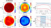 |
Fig. 12 SR map of the two approaches under (a) six GSs and (b) three GSs on the D/r0 = 35 testing sets, (c) SR curves of various lines of sight of two approaches for a different GS number on the D/r0 = 35 testing sets, (d) Comparison of whole FOV average SR between AT-ResNet and MT for a different GS number. |
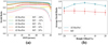 |
Fig. 13 (a) SR curves of various lines of sight. (b) Whole FOV average SR of AT-ResNet and MT under different height offsets for the turbulence layer. |
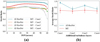 |
Fig. 14 (a) SR curves of various lines of sight. (b) Whole FOV average SR of AT-ResNet and MT under additional conditions for the turbulence layer. |
3.6 Robustness to detection noise
The dominant noise in SH WFS detection images is photon noise and charge-coupled device (CCD) readout noise. Photon noise follows a Poisson distribution, while CCD noise follows a Gaussian distribution. We added photon noise and CCD readout noise to SH WFS images to simulate the impact of detection noise. The formula for calculating the signal-to-noise ratio is given in Eq. (10). Photon noise with a signal-to-noise ratio of 30~50 dB and CCD readout noise with a signal-to-noise ratio of 42~45 dB were randomly added to SH WFS images, and the total signal-to-noise ratio was 30~42 dB,
![$\[S / N=10 \cdot \lg \left(\frac{\sum_j I_j^2}{\sum_j N_j^2}\right),\]$](/articles/aa/full_html/2024/07/aa49788-24/aa49788-24-eq26.png) (10)
(10)
where S/N is the signal-to-noise ratio, Ij is the SH WFS image, and Nj is the noise.
AT-ResNet was retrained under noisy conditions. These two methods were tested under noisy and noise-free conditions, and the results are shown in Fig. 16. Noise can affect the slope calculation of each SH WFS subaperture, thereby affecting the wavefront reconstruction accuracy in multiple GSs directions, and thus affecting the reconstruction accuracy of the whole FOV three-dimensional wavefront aberrations. The results show that the accuracy of the MT approach is significantly affected under noisy conditions. As the turbulence intensity increases, the impact of noise on the aberration detection accuracy becomes more obvious. Neural networks can extract effective feature information from large datasets and filter out the noise. Therefore, AT-ResNet maintains a consistent accuracy and performs very well under noisy conditions. It shows an extremely high robustness to detection noise.
Atmospheric subdivision results with additional turbulence layers.
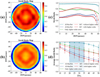 |
Fig. 15 SR map of (a) AT-ResNet and (b) MT on the D/r0 = 35 testing sets. (c) SR curves of various lines of sight of two approaches with a higher-order turbulence aberration on the D/r0 = 35 testing sets. (d) Comparison of the whole FOV average SR between AT-ResNet and MT with a higher-order turbulence aberration. |
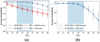 |
Fig. 16 (a) Comparison of the two approaches under noisy conditions, (b) Enlarged version of the AT-ResNet results. |
4 Conclusion
In order to address the nonuniform accuracy of the traditional modal tomography approach in the whole FOV of an atmospheric turbulence wavefront aberration reconstruction, we employed a deep-learning-based approach to reconstruct the three-dimensional atmospheric turbulence wavefront aberration. A comprehensive analysis was conducted on multiple influencing factors involved in the practical application of the MCAO technology. We proposed AT-ResNet to address the atmospheric tomography problem. This network can directly reconstruct the wavefronts of multiple turbulence layers based on the SH WFS detection images from multiple GS directions. Under D/r0 = 10~50 conditions, AT-ResNet consistently achieves an average SR above 0.82 in the whole FOV, outperforming MT. This advantage is particularly obvious under strong turbulence intensity conditions and at the edge of the FOV with a low GS coverage. AT-ResNet demonstrates a certain robustness to variations in the turbulence layer distribution. For a turbulence layer height offset ranging from −20% to 20% and additional turbulence layer cases, its average SR of the whole FOV is also superior to that of the MT approach. Although AT-ResNet does not exhibit a significant advantage over MT when higher-order turbulence aberrations are present, subsequent improvements can alleviate the impact caused by the modal aliasing error, while MT is incapable of eliminating the impact of the modal aliasing error. AT-ResNet also exhibits excellent robustness to detection noise, maintaining a highly stable three-dimensional wavefront aberration detection accuracy under noisy conditions. With a reduction of half the number GSs, the MT approach becomes not applicable, while AT-ResNet only exhibits a noticeable performance degradation under strong turbulence conditions. Moreover, AT-ResNet demonstrates superior performance under three GSs compared to the MT under six GSs, which provides a substantial advantage in practical applications.
The performance of AT-ResNet is significantly superior performance compared to that of MT under different atmospheric turbulence conditions and in various situations involved in the practical application of the MCAO technology. This deep-learning-based method greatly improves the three-dimensional atmospheric turbulence wavefront aberration detection accuracy and achieves a highly uniform and high precision atmospheric turbulence wavefront aberration detection over the large FOV, which is of great significance to the development and application of the MCAO technology. However, there are still some points of this method that can be improved further. First, we only considered the case when the number of estimated turbulence layers is equal to the number of DMs. However, it is also feasible to estimate turbulence layers that exceed the number of DMs. We can generate more turbulence layers than DMs and train the network to directly estimate the Zernike coefficients of multiple turbulence layers. Then, the DM shapes can be determined based on multiple turbulence layers using the approach of Ramlau & Rosensteiner (2012). In future research, we will extend this method to estimate turbulence layers that exceed the number of DMs. Second, this method does not consider the impact of higher-order turbulence aberrations during the training process, resulting in a significant performance degradation when encountering higher-order turbulence aberrations. Future research will introduce higher-order turbulence aberrations into the training sets to alleviate the effects of the modal aliasing error on the algorithm. The last point is that this method has only been validated in a simulated open-loop case and has not been further verified on an experimental platform. In the follow-up work, the experimental validation will be conducted on a closed-loop MCAO experimental optics system, and the method will be further improved for extended objects. Moreover, this method will also be optimized for the MCAO system at the New Vacuum Solar Telescope of the Yunnan Astronomical Observatory to obtain high-resolution images with large FOVs.
Acknowledgements
This work was supported by the National Natural Science Foundation of China (12103057); Youth Innovation Promotion Association, Chinese Academy of Sciences (Nos. 2022386, 2021357); Frontier Research Fund of Institute of Optics and Electronics, Chinese Academy of Sciences (C21K002).
References
- Beckers, J. M. 1988, in Very Large Telescopes and their Instrumentation, 2, 30, 693 [NASA ADS] [Google Scholar]
- Ellerbroek, B. L., & Vogel, C. R. 2009, Inverse Probl., 25, 063001 [NASA ADS] [CrossRef] [Google Scholar]
- Fried, D. L. 1982, J. Opt. Soc. Am., 72, 52 [CrossRef] [Google Scholar]
- Fusco, T., Conan, J.-M., Michau, V., Mugnier, L. M., & Rousset, G. 1999, in Propagation and Imaging through the Atmosphere III, 3763, eds. M. C. Roggemann, & L. R. Bissonnette (International Society for Optics and Photonics SPIE), 125 [NASA ADS] [CrossRef] [Google Scholar]
- Fusco, T., Conan, J.-M., Michau, V., Rousset, G., & Assemat, F. 2001a, in Atmospheric Propagation, Adaptive Systems, and Laser Radar Technology for Remote Sensing, 4167, eds. J. D. Gonglewski, G. W. Kamerman, A. Kohnle, U. Schreiber, & C. Werner (International Society for Optics and Photonics SPIE), 168 [NASA ADS] [CrossRef] [Google Scholar]
- Fusco, T., Conan, J.-M., Rousset, G., Mugnier, L. M., & Michau, V. 2001b, J. Opt. Soc. Am. A, 18, 2527 [NASA ADS] [CrossRef] [Google Scholar]
- Golub, G. H., Heath, M., & Wahba, G. 1979, Technometrics, 21, 215 [Google Scholar]
- Gerchberg, R., & Saxton, W. 1972, Optik, 35, 237 [Google Scholar]
- Gonsalves, R. A. 1982, Opt. Eng., 21, 215829 [NASA ADS] [CrossRef] [Google Scholar]
- Guo, H., Xu, Y., Li, Q., et al. 2019, Sensors, 19 [Google Scholar]
- Guo, Y., Wu, Y., Li, Y., Rao, X., & Rao, C. 2021, MNRAS, 510, 4347 [Google Scholar]
- Guo, Y., Zhong, L., Min, L., et al. 2022, Opto-Electron. Adv., 5, 200082 [Google Scholar]
- He, B. 2016, PhD thesis, Changchun Institute of Optics, Fine Mechanics and Physics, Chinese Academy of Sciences [Google Scholar]
- He, K., Zhang, X., Ren, S., & Sun, J. 2016, in 2016 IEEE Conference on Computer Vision and Pattern Recognition (CVPR), 770 [Google Scholar]
- Hou, Q., Zhou, D., & Feng, J. 2021, in Proceedings of the IEEE/CVF Conference on Computer Vision and Pattern Recognition (CVPR), 13713 [Google Scholar]
- Hu, L., Hu, S., Gong, W., & Si, K. 2019, Opt. Express, 27, 33504 [NASA ADS] [CrossRef] [Google Scholar]
- Hu, L., Hu, S., Gong, W., & Si, K. 2020, Opt. Lett., 45, 3741 [NASA ADS] [CrossRef] [Google Scholar]
- Hufnagel, R. 1974, Digest of Technical Papers – Topical Meeting on Optical Propagation Through Turbulence (Optical Society of America) [Google Scholar]
- Ioffe, S., & Szegedy, C. 2015, in Proceedings of Machine Learning Research, 37, Proceedings of the 32nd International Conference on Machine Learning, eds. F. Bach, & D. Blei (Lille, France: PMLR), 448 [Google Scholar]
- Jiang, W. 2018, Opto-Electronic Engineering, 45, 170489 [Google Scholar]
- Jordan, M. I., & Mitchell, T. M. 2015, Science, 349, 255 [CrossRef] [Google Scholar]
- Kingma, D. P., & Ba, J. 2014, arXiv e-prints [arXiv:1412.6980] [Google Scholar]
- LeCun, Y., Bengio, Y., & Hinton, G. 2015, Nature, 521, 436 [Google Scholar]
- Ma, N., Zhang, X., & Sun, J. 2020, in Computer Vision–ECCV 2020: 16th European Conference, Glasgow, UK, August 23–28, 2020, Proceedings, Part XI 16 (Springer), 351 [Google Scholar]
- Marchetti, E., Brast, R., Delabre, B., et al. 2007, in Adaptive Optics: Analysis and Methods/Computational Optical Sensing and Imaging/Information Photonics/Signal Recovery and Synthesis Topical Meetings on CD-ROM (Optica Publishing Group), AMA2 [Google Scholar]
- Nair, V., & Hinton, G. E. 2010, in Proceedings of the 27th international conference on machine learning (ICML-10), 807 [Google Scholar]
- Nishizaki, Y., Valdivia, M., Horisaki, R., et al. 2019, Opt. Express, 27, 240 [NASA ADS] [CrossRef] [Google Scholar]
- Noll, R. J. 1976, J. Opt. Soc. Am., 66, 207 [Google Scholar]
- Orban de Xivry, G., Quesnel, M., Vanberg, P.-O., Absil, O., & Louppe, G. 2021, MNRAS, 505, 5702 [NASA ADS] [CrossRef] [Google Scholar]
- Osborn, J., Guzman, D., de Cos Juez, F. J., et al. 2014, MNRAS, 441, 2508 [NASA ADS] [CrossRef] [Google Scholar]
- Ragazzoni, R., Marchetti, E., & Rigaut, F. 1999, A&A, 342, L53 [NASA ADS] [Google Scholar]
- Ramlau, R., & Rosensteiner, M. 2012, Inverse Probl., 28, 095004 [NASA ADS] [CrossRef] [Google Scholar]
- Ramlau, R., & Saxenhuber, D. 2016, Inverse Probl. Imag., 10, 781 [CrossRef] [Google Scholar]
- Rao, C., Zhang, L., Kong, L., et al. 2018, Sci. China Phys. Mech. Astron., 61, 089621 [CrossRef] [Google Scholar]
- Rosensteiner, M., & Ramlau, R. 2013, J. Opt. Soc. Am. A, 30, 1680 [NASA ADS] [CrossRef] [Google Scholar]
- Stadler, B., & Ramlau, R. 2022, J. Astron. Telescopes Instrum. Syst., 8, 021503 [NASA ADS] [Google Scholar]
- Vogel, C. R., & Yang, Q. 2006, Opt. Express, 14, 7487 [NASA ADS] [CrossRef] [Google Scholar]
- Wallner, E. P. 1994, in Adaptive Optics in Astronomy, 2201, eds. M. A. Ealey, & F. Merkle (International Society for Optics and Photonics SPIE), 110 [NASA ADS] [CrossRef] [Google Scholar]
- Yang, Q., Vogel, C. R., & Ellerbroek, B. L. 2006, Appl. Opt., 45, 5281 [NASA ADS] [CrossRef] [Google Scholar]
- Yudytskiy, M. 2014, PhD thesis, Johannes Kepler University Linz, Austria [Google Scholar]
- Yudytskiy, M., Helin, T., & Ramlau, R. 2014, J. Opt. Soc. Am. A, 31, 550 [NASA ADS] [CrossRef] [Google Scholar]
All Tables
All Figures
|
Fig. 1 Schematic diagram of the three-dimensional wavefront aberration detection. |
| In the text | |
|
Fig. 2 Schematic diagram of the GS detection in multiple turbulence layers. |
| In the text | |
|
Fig. 3 Footprints of six GSs in three turbulence layers. |
| In the text | |
|
Fig. 4 Panel a: standard input: SH WFS images of six GS directions. Panels b and c: standard output: three-layer phase screen wavefront. |
| In the text | |
|
Fig. 5 Structure of (a) AT-ResNet. The schematic diagram of (b) the FReLU function, (c) the CoordAttention, and (d) ResBlock. |
| In the text | |
|
Fig. 6 Average results of AT-ResNet for all testing sets. Panel a: SR curves of various lines of sight. Panel b: whole FOV SR map. |
| In the text | |
|
Fig. 7 Reconstruction results of three-layer phase screens for one testing set using AT-ResNet and MT. |
| In the text | |
|
Fig. 8 (a) Comparison of SR curves between the two methods from one testing set. The whole FOV SR map of (b) AT-ResNet and (c) MT from one testing set. |
| In the text | |
|
Fig. 9 Comparison of AT-ResNet and MT for (a) D/r0 = 20 and (b) D/r0 = 35 conditions. |
| In the text | |
|
Fig. 10 SR curves of various lines of sight of (a) AT-ResNet and (b) MT under different turbulence intensity conditions. (c) Comparison of the whole FOV average SR between AT-ResNet and MT under different turbulence intensity conditions. |
| In the text | |
|
Fig. 11 Footprints of three GSs in three turbulence layers. |
| In the text | |
|
Fig. 12 SR map of the two approaches under (a) six GSs and (b) three GSs on the D/r0 = 35 testing sets, (c) SR curves of various lines of sight of two approaches for a different GS number on the D/r0 = 35 testing sets, (d) Comparison of whole FOV average SR between AT-ResNet and MT for a different GS number. |
| In the text | |
|
Fig. 13 (a) SR curves of various lines of sight. (b) Whole FOV average SR of AT-ResNet and MT under different height offsets for the turbulence layer. |
| In the text | |
|
Fig. 14 (a) SR curves of various lines of sight. (b) Whole FOV average SR of AT-ResNet and MT under additional conditions for the turbulence layer. |
| In the text | |
|
Fig. 15 SR map of (a) AT-ResNet and (b) MT on the D/r0 = 35 testing sets. (c) SR curves of various lines of sight of two approaches with a higher-order turbulence aberration on the D/r0 = 35 testing sets. (d) Comparison of the whole FOV average SR between AT-ResNet and MT with a higher-order turbulence aberration. |
| In the text | |
|
Fig. 16 (a) Comparison of the two approaches under noisy conditions, (b) Enlarged version of the AT-ResNet results. |
| In the text | |
Current usage metrics show cumulative count of Article Views (full-text article views including HTML views, PDF and ePub downloads, according to the available data) and Abstracts Views on Vision4Press platform.
Data correspond to usage on the plateform after 2015. The current usage metrics is available 48-96 hours after online publication and is updated daily on week days.
Initial download of the metrics may take a while.