| Issue |
A&A
Volume 682, February 2024
|
|
|---|---|---|
| Article Number | A175 | |
| Number of page(s) | 6 | |
| Section | Celestial mechanics and astrometry | |
| DOI | https://doi.org/10.1051/0004-6361/202348082 | |
| Published online | 23 February 2024 | |
Bayesian test of Brans–Dicke theories with planetary ephemerides: Investigating the strong equivalence principle
1
Géoazur, Université Côte d’Azur, Observatoire de la Côte d’Azur, CNRS,
250 Av. A. Einstein,
06250
Valbonne,
France
e-mail: This email address is being protected from spambots. You need JavaScript enabled to view it.
2
Université Côte d’Azur, Observatoire de la Côte d’Azur, CNRS,
Artemis, bd. de l’Observatoire,
06304
Nice,
France
3
Bureau des Affaires Spatiales,
2 rue du Gabian,
98000
Monaco
4
IMCCE, Observatoire de Paris, PSL University, CNRS,
77 Av. Denfert-Rochereau,
75014
Paris,
France
Received:
27
September
2023
Accepted:
29
November
2023
Abstract
Aims. We are testing the Brans–Dicke class of scalar tensor theories with planetary ephemerides.
Methods. In this work, we apply our recently proposed Bayesian methodology to the Brans–Dicke case, with an emphasis on the issue of the strong equivalence principle (SEP).
Results. We use an MCMC approach coupled to full, consistent planetary ephemeris construction (from point-mass body integration to observational fit) and compare the posterior distributions obtained with and without the introduction of potential violations of the SEP.
Conclusions. We observe a shift in the confidence levels of the posteriors obtained. We interpret this shift as marginal evidence that the effect of violation of the SEP can no longer be assumed to be negligible in planetary ephemerides with the current data. We also notably report that the constraint on the Brans–Dicke parameter with planetary ephemerides is getting closer to the figure reported from the Cassini spacecraft alone, and also to the constraints from pulsars. We anticipate that data from future spacecraft missions, such as BepiColombo, will significantly enhance the constraints based on planetary ephemerides.
Key words: gravitation / methods: statistical / celestial mechanics / ephemerides
© The Authors 2024
 Open Access article, published by EDP Sciences, under the terms of the Creative Commons Attribution License (https://creativecommons.org/licenses/by/4.0), which permits unrestricted use, distribution, and reproduction in any medium, provided the original work is properly cited.
This article is published in open access under the Subscribe to Open model. This email address is being protected from spambots. You need JavaScript enabled to view it. to support open access publication.
1 Introduction
Planetary ephemerides have evolved over the years in line with improvements in the observational accuracy of the astrometry of planets and natural satellites using the navigation tracking of these systems. The motion of the celestial bodies in our Solar System can be solved directly by integrating their equations of motion numerically. The improved accuracy in measurements of observables from space missions (e.g. Cassini-Huygens, Mars Express, BepiColombo, Juice, etc.) makes the Solar System a suitable environment for testing general relativity theory (GRT) as well as alternative theories of gravity by means of Solar System ephemerides. For a detailed review regarding the use of planetary ephemerides for testing gravity, we refer to Fienga & Minazzoli (2024). Since 2003, the INPOP (Intégrateur Numérique Planétaire de l’Observatoire de Paris) planetary ephemerides have been developed (Fienga et al. 2008, 2009) with numerical integration of the Einstein-Infeld-Hoffmann equations of motion proposed by Moyer (2003), and by fitting the parameters of the dynamical model to the most accurate planetary observations following Soffel et al. (2003). In the present work, we use the INPOP21a planetary ephemerides (Fienga et al. 2021), which benefit from the latest Juno and Mars orbiter tracking data up to 2020, and from radio-science observations from space missions such as Cassini-Huygens, Mars Express, and Venus Express. Moreover, a fit of the Moon–Earth system to Lunar Laser Ranging (LLR) observations up to 2020 is included. The dynamical modelling used in INPOP21a takes into account the eight planets of the Solar System, as well as Pluto, the Moon, the asteroids, the Kuiper belt, the Sun oblateness, and the Lense–Thirring effect. We refer the reader to Fienga et al. (2021) for a detailed review of this version of INPOP. In recent years, the post-Newtonian (PPN) parameters have already been tested with planetary ephemerides (Fienga & Minazzoli 2024). However, previous derivations did not take into account the potential violation of the strong equivalence principle (SEP) owing to its assumed small impact on the ephemerides. In other words, the effect of the gravitational self-energy of the planets violating the SEP was not implemented in the equations of motion. This decision was based on order-of-magnitude derivations that indicated that the effect was not deemed significant given the accuracy of the previous ephemerides.
Nevertheless, almost all alternative theories predict a violation of the SEP – that is, they predict that bodies with different self-gravitating energies fall differently in a given gravitational field (Nordtvedt 1968a,b; Will 2018). In the PPN framework, this effect is parameterized by the Nordtvedt parameter η – see Eq. (6) – in reference to Nordtvedt (1968a,b), and η = 0 in general relativity. Therefore, it was only a matter of time before planetary ephemerides reached a level of accuracy that necessitated that this effect be accounted for in the integration of the equations of motion.
In the present work, we implement the whole set of relevant equations in the Brans–Dicke case – including the effects of the predicted violation of the SEP. We use the recent work of Bernus et al. (2022), who derived the whole phenomenology of Einstein-dilaton theories, and restrict our analysis to the one-parameter family that corresponds to Brans–Dicke theories. As we show in Sect. 2.1, one of the reasons for caution is that there is a potential ambiguity regarding the types of mass (gravitational or inertial) that appear in various equations, namely the equation of motion, the Shapiro delay, and the definition of the barycenter. We therefore start from a consistently derived phenomenology.
The motivation for investigating violations of the SEP in planetary ephemerides within the relatively limited framework of Brans–Dicke theories is two-fold. Firstly, as explained in a recent review (Fienga & Minazzoli 2024), because of the correlations between the parameters of the Solar System (masses, initial conditions, shape, etc.) and the theoretical parameters that parameterize deviations from the laws of general relativity (e.g. PPN parameters), it is somewhat difficult to produce statistically robust tests of alternative theories to general relativity. Fienga & Minazzoli (2024) indeed notably argue that one should focus on each set of theories in a consistent manner, and this is our aim for the present study. Secondly, a robust statistical Bayesian methodology was recently developed and used to test a potential Yukawa suppression of the Newtonian potential in the Solar System (Mariani et al. 2023b). It is interesting to apply this new methodology to other alternative phenomenologies. However, it is only feasible to apply such an approach to phenomenologies that have just one theoretical parameter to be tested. Therefore, if the methodology is applied to scalar-tensor theories, one must restrict the study to the Brans–Dicke case.
2 Dynamical and statistical formalism
2.1 Gravitational framework
A discrepancy in the free fall of particles with differing compositions in a particular gravitational field would signify a violation of the weak equivalence principle (WEP). Meanwhile, a deviation for extended bodies with distinct gravitational self-energies would indicate a breach of the gravitational weak equivalence principle (GWEP). The latter forms a component of the SEP, as delineated by Will (2018). In all instances, through planetary ephemerides, our objective is to verify the universality of free fall (UFF), or, in other words, to confirm whether all bodies, regardless of their characteristics, experience identical rates of fall in a given gravitational field.
The violations of both the WEP and GWEP share a characteristic feature: at the Newtonian level, their equations of motion are expressed as follows (Bernus et al. 2022; Minazzoli & Hees 2016):
 (1)
(1)
where aT is the coordinate acceleration of body T (whereas the letter A is used as index for the other bodies); rAT is the relative position of body T with respect to A; rAT = |rAT|, with  being the body A gravitational parameter; and δT and δAT are coefficients that depend on the composition of the bodies T and A for the case of the violation of the WEP only. The most general post-Newtonian phenomenology for Einstein-dilaton theories was derived by Bernus et al. (2022), and depends on several parameters that are related to the coupling between matter and gravity. Because the exploration of a high-dimensional theoretical space is very demanding in terms of computation time, a reduction of the number of parameters was made owing to the roughly similar compositions of the celestial bodies, and a simple rejection sampling was applied to the solutions of the ephemerides in order to estimate the constraints of the theoretical parameters.
In what follows, we use an opposing strategy: given the recent very effective Bayesian methodology that is well suited to the one-parameter family of theories, we reduce the general Einstein-dilaton action to the case of only one parameter, effectively recovering the Brans–Dicke theory, and we apply the Bayesian methodology to this case.
Following Bernus et al. (2022), the equation of motion of the Brans–Dicke special case corresponds to
![Mathematical equation: $\eqalign{ & {a_{\rm{T}}} = - \sum\limits_{{\rm{A}} \ne {\rm{T}}} {{{{\mu _{\rm{A}}}} \over {r_{{\rm{AT}}}^3}}} {r_{{\rm{AT}}}}\left( {1 + {\delta _{\rm{T}}}} \right) - \sum\limits_{{\rm{A}} \ne {\rm{T}}} {{{{\mu _{\rm{A}}}} \over {r_{{\rm{AT}}}^3{c^2}}}} {r_{{\rm{AT}}}}\left\{ {\gamma v_{\rm{T}}^2 + (\gamma + 1)\upsilon _{\rm{A}}^2} \right. \cr & \,\,\,\,\,\,\,\,\,\, - 2(1 + \gamma ){\upsilon _{\rm{A}}} \cdot {\upsilon _{\rm{T}}} - {3 \over 2}{\left( {{{{r_{{\rm{AT}}}} \cdot {\upsilon _{\rm{A}}}} \over {{r_{{\rm{AT}}}}}}} \right)^2} - {1 \over 2}{r_{{\rm{AT}}}} \cdot {a_{\rm{A}}} - 2\gamma \sum\limits_{B \ne T} {{{{\mu _{\rm{B}}}} \over {{r_{TB}}}}} \left. { + \sum\limits_{B \ne A} {{{{\mu _{\rm{B}}}} \over {{r_{{\rm{AB}}}}}}} } \right\} \cr & \,\,\,\,\,\,\,\,\,\,\, + \sum\limits_{{\rm{A}} \ne {\rm{T}}} {{{{\mu _{\rm{A}}}} \over {{c^2}r_{{\rm{AT}}}^3}}} \left[ {2(1 + \gamma ){r_{{\rm{AT}}}} \cdot {\upsilon _{\rm{T}}} - (1 + 2\gamma ){r_{{\rm{AT}}}} \cdot {\upsilon _{\rm{A}}}} \right] \cr & \,\,\,\,\,\,\,\,\,\,\,\left( {{\upsilon _{\rm{T}}} - {\upsilon _{\rm{A}}}} \right) + {{3 + 4\gamma } \over 2}\sum\limits_{{\rm{A}} \ne {\rm{T}}} {{{{\mu _{\rm{A}}}} \over {{c^2}{r_{{\rm{AT}}}}}}} {a_{\rm{A}}}, \cr} $](/articles/aa/full_html/2024/02/aa48082-23/aa48082-23-eq3.png) (2)
(2)
where δT and the parameter γ depend only on a universal coupling constant α0, such that
 (3)
(3)
and
 (4)
(4)
with
 (5)
(5)
where RT is the radius of the planet T. This implies that the Nordtvedt parameter in this case is
 (6)
(6)
The Shapiro delay is also modified and is now such that the whole coordinate propagation time between an emitter and a receiver (tr − te) reads as follows:
 (7)
(7)
where R is the coordinate Euclidean distance between the emitter and the receiver. Another way to formulate the Shapiro delay is in terms of the inertial gravitational parameter,
 (8)
(8)
where  is the inertial mass of the body T, such that
 (9)
(9)
In other words, the Shapiro delay is sensitive to the iner-tial masses, whereas the equation of motion depends on the gravitational masses.
Equally importantly, the definition of the Solar System barycenter (SSB) also involves the inertial gravitational parameter  . Indeed, from the Lagrangian formulation of the equations of motion, Bernus et al. (2022) show that the following barycenter constant vector is a first integral of the equations of motion,
 (10)
(10)
where
 (11)
(11)
are the coordinates of the relativistic barycenter of the system and
 (12)
(12)
is the velocity of the barycenter motion. h is the conserved energy – whose value does not affect what follows but can be found in Bernus et al. (2022) – and P is the conserved linear momentum, which reads
![Mathematical equation: $\matrix{ {} \hfill & {\mathop {P = \sum }\limits_{\rm{A}} {p_{\rm{A}}}} \hfill \cr {} \hfill & {\mathop { = \,\sum }\limits_{\rm{A}} \mu _{\rm{A}}^i{\upsilon _{\rm{A}}}\left[ {1 + {1 \over {2{c^2}}}\left( {\upsilon _{\rm{A}}^2 - \mathop \sum \limits_{B \ne A} {{{\mu _{\rm{B}}}} \over {{r_{{\rm{AB}}}}}}} \right)} \right]} \hfill \cr {} \hfill & { - {1 \over {2{c^2}}}\mathop \sum \limits_{\rm{A}} \mathop \sum \limits_{B \ne A} {{{\mu _{\rm{A}}}{\mu _{\rm{B}}}} \over {{r_{{\rm{AB}}}}}}\left( {{n_{{\rm{AB}}}} \cdot {\upsilon _{\rm{A}}}} \right){n_{{\rm{AB}}}}.} \hfill \cr } $](/articles/aa/full_html/2024/02/aa48082-23/aa48082-23-eq16.png) (13)
(13)
In this work, we implemented Eqs. (2) and (7) in the INPOP planetary ephemerides numerical integration of the planet equations of motion and its adjustment to observations, whereas – because the system has a conserved linear momentum – the equation for the SSB (defined with the inertial gravitational parameter) is integrated once at J2000, which is the initial date of integration for INPOP ephemerides. We used INPOP21a for this test, as in Mariani et al. (2023b,a), by considering different values of α0 and the changes this induces in γ and η. The obtained results are presented in Sect. 3.2 in terms of γ, while Sect. 2.2 explains the statistical method.
To assess the effect of considering the potential violation of the GWEP (and therefore of the SEP) in planetary ephemerides, we constrained the value of γ either assuming that η = 0 (in Sect. 3.1) – as was the case in previous planetary ephemerides – or assuming that η = −(1 − γ) (in Sect. 3.2).
2.2 Statistical aspects
Starting from Fienga et al. (2015; also in Di Ruscio et al. 2020 and Fienga et al. 2020), several tools have been used to determine the goodness of the INPOP fit with respect to modifications in the equations of motion or in the framework of the ephemeris, as well as the observations. Within this context, the computation of the INPOP χ2 plays a role in determining which model (or which data) leads to a significant improvement of the ephemeris computation. In the present work, the computation of χ2 is the output – for a given value of γ – of the INPOP iterative fit, that is, after the adjustment of all its astronomical parameters (see Mariani et al. 2023b,a; Bernus et al. 2019). The χ2(γ) is computed following (14)
 (14)
(14)
where γ is a fixed value, k are the astronomical parameters fitted with INPOP, Nobs is the number of observations, the function ɡi represents the computation of observables, the vector  is the vector of observations and σi are the observational uncertainties. The goal of the methodology applied is to obtain a posterior for the parameter γ. The general pipeline used to obtain such a posterior is similar to that adopted by Mariani et al. (2023a,b). We compute the value χ2(γ) (see Eq. (14)) for several different values of γ, spreading over our domain of interest. For any given γ, the value χ2(γ) is obtained as an outcome of the full INPOP iterative adjustment, with γ fixed. In this way, the astronomical parameters are adjusted with the least-squares procedure, whereas γ is a fixed value. Fixing the value of γ is necessary as it ensures the γ contribution to the dynamics, avoiding high correlations between γ and the other astronomical parameters k (see Anderson et al. 1978; Bernus et al. 2019) for further details about correlation problem). In order to produce the posterior, we use a Markov chain Monte Carlo (MCMC) method, the Metropolis–Hastings (MH) algorithm. In order to produce the MCMC, it is necessary to evaluate the likelihood, sequentially, and therefore the χ2, for thousands of different values of γ (see Mariani et al. 2023a for further details). As the computation of χ2(γ) is expensive in terms of time, it becomes difficult to run the MCMC with the χ2 direct calculation. In order to overcome the problem of computation time, we apply a Gaussian process regression (GPR) to interpolate among the values (γ, χ2(γ)) already computed beforehand. Starting from this set of points, we obtain, thanks to the GPR, a function
  , together with an uncertainty relative to the possible error of interpolation. The regression
  is necessary to run the MH algorithm, which has, as an outcome, the posterior density. Moreover, an a priori density distribution has to be provided for the parameter of interest (i.e. γ) to sample with the MCMC from the posterior. We used a uniform prior distribution for γ. The MH algorithm is based on the idea that the drawings from the posterior distribution are done sequentially and according to a random acceptance process. The outcome of the algorithm is a sequence of random samples from the posterior (this sequence is the Markov chain) and its equilibrium distribution is the posterior itself. At each step of the algorithm, one new element of the sequence is computed and proposed, and is accepted or rejected. The acceptance/rejection step is random: this randomness is determined by a certain probability (which changes at each step) based on the last accepted element of the sequence as well as the likelihood of the last element and of the new candidate element.
3 Results
3.1 Limit on γ without SEP violation
In order to evaluate the impact of the method within a well-known context Mariani et al. (2023a), we first estimated the possible violation of general relativity by considering 1 − γ ≠ 1 without considering possible SEP violation (i.e. η = 0). In this case, the terms δT in Eq. (2) and δA in Eq. (7) vanish and only the terms with γ remain. With this configuration, our results are comparable to classical conjunction tests like the one obtained during the Cassini interplanetary phase when the radio-science signal of the Cassini s/c grazed the Sun before reception on earth. During this conjunction, the Shapiro delay is at its maximum and Bertotti et al. (2003) deduced the best constraint on γ so far with a global fit of s/c orbit parameters and γ. As this part of the mission (interplanetary phase) is supposed to be the least affected by complex gravitational interactions or maneuvers, the determination is in principle the most accurate and the least affected by biases or noise. Because of the estimation method (least square), the Bertotti et al. (2003) constraint, 1 − γ = (−2.1 ± 2.3) × 10−5, is given at 1σ, assuming a Gaussian distribution of the noise. Two main differences between our approach and the results obtained by Bertotti et al. (2003) have to be stressed. First, by construction of our model, only values of γ where 1 − γ > 0 are tested. Once we compare our results with Bertotti et al. (2003), we have to compare with the absolute value of their interval as it is represented in Fig. 1. Second, we use a Bayesian approach using a uniform prior with a maximum value for 1 − γ of 15 × 10−5 and providing a posterior distribution of acceptable 1 − γ values, as discussed in Sect. 2.2. In this context, for comparisons of results, it is important to consider the confidence level (C.L.) deduced from the posteriors. In Fig. 1 and Table 1, we see the limit of about 4.4 × 10⁻⁵ at 66.7% C.L. (1σ) of the ‖1 − γ‖ interval deduced from Bertotti et al. (2003; black dashed line on Fig. 1) and in yellow, the posterior distribution of ‖1 − γ‖ obtained with this work. At 99.7% C.L., we obtain a limit of 2.5 × 10⁻⁵ (red dot-dashed line on Fig. 1) and of about 1.73 × 10⁻⁵ at 66.7% C.L. (blue dotted line on Fig. 1). It is interesting to note, at this stage, that the limits we obtain are of the same order of magnitude as those obtained by Bertotti et al. (2003). However, we stress that these results were obtained while exploring only γ values smaller than 1.
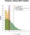 |
Fig. 1 Posterior distributions without SEP violation. Yellow: Posterior distribution for 1 − γ without the implementation of the SEP violation. Green: Absolute value of the simulated posterior for the determination of 1 − γ with Cassini. Red line (dot-dashed): 99.7% C.L. ((1 − γ) = 2.50 × 10⁻⁵). Blue line (dotted): 66.7% C.L. ((1 − γ) = 1.73 × 10⁻⁵). Purple line (dashed): 95% C.L. ((1 − γ) = 2.40 × 10⁻⁵). The prior for (1 − γ) is a uniform prior between 0 and 15 × 10−5. Solid black line: Absolute value of Cassini central value estimation ((1 − γ) = −2.1 × 10⁻⁵). Dashed black line: Upper bound estimation from Cassini at 1σ C.L. |
3.2 Limit on γ and α0 with SEP violation
After considering the results of an exploration of the 1 − γ without SEP violation, we now switch to the full Brans–Dicke formalism with SEP violation as described in Sect. 2.1. We used the method described in Sect. 2.2 for the determination of acceptable values for the parameter α0. Figure 2 shows the posterior of 1 − γ and the deduced α0 from Eq. (3). At 99.7 % C.L., we obtain a limit on ||1 − γ|| of about 2.83 × 10⁻⁵, leading to a constraint on α0 of about 3.76 × 10⁻³. From the constraint on α0 and on γ, one can deduce limits for the Nordtvedt parameter η = γ − 1. As given on Table 1, at 99.7 % C.L., η > −2.83 × 10⁻⁵, at 95 % C.L., η > −2.70 × 10⁻⁵, and at 66.7 % C.L., η > −1.92 × 10⁻⁵. We stress that these constraints are only for η < 0 (see Eq. (6)). Different values of η can be compared with these results (see Table 1) but all are deduced from a direct fit either of the s/c orbit, such as with Genova et al. (2018), or of the Earth–Moon system (Viswanathan et al. 2018).
In Genova et al. (2018), η is obtained during the orbit determination of the s/c Messenger orbiting Mercury. In the global fit, in addition to orbit determination parameters, the PPN parameter β, the Sun oblateness J2, and η are also estimated. PPN γ is fixed to the Bertotti et al. (2003) value.
As discussed in Fienga & Minazzoli (2024), the four parameters are strongly correlated, with or without the use of the Nordtvedt relation,
 (15)
(15)
For comparison, in Table 1, we propose some values found in the literature obtained with very different methods. In particular, we consider the thresholds obtained with Bernus et al. (2022) in the context of the Einstein-dilaton theories, which can be seen as a generalisation of the Brans–Dicke scalar–tensor theories. Indeed, in this case, coupling between matter and the scalar field is introduced and can take either a linear or a non-linear form. In Bernus et al. (2022), limits on the universal coupling α0 have been obtained using planetary ephemerides (INPOP19a) together with constraints for the gaseous and the telluric planets, αG and αT, respectively. The comparison between the limit obtained for α0 in this work and that from Bernus et al. (2022) is not straight-forward, as in our case, we have αG = αT = 0.
4 Discussion
4.1 The equivalence principle
It is interesting to note that the limit obtained for 1 − γ in the BD framework with the SEP violation is larger than that obtained without the SEP violation (see Fig. 1). We interpret this as marginal evidence that, at the level of accuracy of current planetary ephemerides, the effect of the SEP violation is no longer negligible. Indeed, adding the effect increases the correlations between γ and planetary parameters, which, here, comes from the additional correlations that exist between δT and planetary parameters (masses, initial conditions, etc.). This leads to the usual reduction in the accuracy of the estimation of the constraint on the theoretical parameter being tested. Indeed, with a greater number of correlations, more freedom is provided with which to better fit the data; this leads to weaker constraints. For a comprehensive discussion about the general issue of correlations between theoretical and planetary parameters, we refer the reader to Fienga & Minazzoli (2024). Also, because we observe that including the SEP violation leads to slightly more stable solutions for the planetary orbits, we believe that including the SEP violation in alternative theories – that is, η ≠ 0 – is more consistent at the dynamical level than not including it.
Results and comparisons.
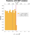 |
Fig. 2 Posterior distribution for 1 − γ and the corresponding values of α0 in the Brans–Dicke framework with the implementation of the SEP violation. Red line (dot-dashed): 99.7% C.L. ((1 − γ) = 2.83 × 10⁻⁵ and α0 = 3.762 × 10⁻³). Blue line (dotted): 66.7% C.L. ((1 − γ) = 1.92 × 10⁻⁵ and α0 = 3.096 × 10⁻³). Purple line (dashed): 95% C.L. ((1 − γ) = 2.70 × 10⁻⁵ and α0 = 3.675 × 10⁻³). The prior for (1 − γ) is a uniform prior between 0 and 15 × 10−5. |
4.2 Conversion in terms of the usual Brans–Dicke parameter ωBD
One can simply convert the constraint on α0 to a constraint on the usual Brans–Dicke parameter ωBD (Will 2014)
 (16)
(16)
Therefore, based on the results given in Table 1, we can derive a 99.7% C.L. with ωBD > 35 382. The limits obtained with the planetary ephemerides in this work are not as stringent as those obtained by Voisin et al. (2020). Indeed, using observations of a pulsar in a triple-star system, Voisin et al. (2020) deduce that ωBD > 130000 although this value depends on the equation of state being assumed for the neutron star, and variation of a few tens of percent is generally found when using different equations of state (Voisin et al. 2020). Hence, constraints from planetary ephemerides are currently less powerful than the best constraints from pulsars. Nevertheless, we anticipate that future spacecraft missions, such as BepiColombo, will significantly improve the constraining power of planetary ephemerides in the near future.
5 Conclusions
In the present paper, we used a recent powerful Bayesian methodolgy developed for a one-parameter theoretical model in order to obtain the latest constraints from planetary ephemerides on the Brans–Dicke theory of gravity. In this context, we find that ‖1 − γ‖ < 1.92 ×10⁻⁵ at the 66.7% C.L., while the previous best Solar System constraints from ranging data of the Cassini spacecraft (Bertotti et al. 2003) on γ led to ‖1 − γ‖ < 4.4 × 10⁻⁵ at 66.7% C.L. At the 99.7% C.L., the new planetary ephemerides constraint reads ‖1 − γ‖ < 2.83 × 10⁻⁵. While this is still inferior to the best constraints from pulsars (Voisin et al. 2020), missions such as BepiColombo should improve this constraint in the near future. We also report marginal evidence suggesting that the effect of the violation of the strong equivalence principle can no longer be assumed to be negligible with the current accuracy of planetary ephemerides.
Acknowledgements
V.M. was funded by CNES (French Space Agency) and UCA EUR Spectrum doctoral fellowship. This work was supported by the French government, through the UCAJEDI Investments in the Future project managed by the National Research Agency (ANR) under reference number ANR-15-IDEX-01. The authors are grateful to the OPAL infrastructure and the Université Côte d’Azur Center for High-Performance Computing for providing resources and support. The authors thank G. Voisin for his useful inputs and discussions. This work was supported by the French group for gravitation and metrology PNGRAM (Programme National Gravitation, Références, Astronomie, Métrologie).
References
- Anderson, J., Keesey, M., Lau, E., Standish, E., & Newhall, X. 1978, Acta Astronautica, 5, 43 [NASA ADS] [CrossRef] [Google Scholar]
- Bernus, L., Minazzoli, O., Fienga, A., et al. 2019, Phys. Rev. Lett., 123, 161103 [Google Scholar]
- Bernus, L., Minazzoli, O., Fienga, A., et al. 2022, Phys. Rev. D, 105, 044057 [NASA ADS] [CrossRef] [Google Scholar]
- Bertotti, B., Farinella, P., & Vokrouhlick, D. 2003, Physics of the Solar System – Dynamics and Evolution, Space Physics, and Spacetime Structure, ASSL, 293 [Google Scholar]
- Di Ruscio, A., Fienga, A., Durante, D., et al. 2020, A&A, 640, A7 [NASA ADS] [CrossRef] [EDP Sciences] [Google Scholar]
- Fienga, A., & Minazzoli, O. 2024, Liv. Rev. Rel., 27, 1 [NASA ADS] [CrossRef] [Google Scholar]
- Fienga, A., Manche, H., Laskar, J., & Gastineau, M. 2008, A&A, 477, 315 [NASA ADS] [CrossRef] [EDP Sciences] [Google Scholar]
- Fienga, A., Laskar, J., Morley, T., et al. 2009, A&A, 507, 1675 [NASA ADS] [CrossRef] [EDP Sciences] [Google Scholar]
- Fienga, A., Laskar, J., Exertier, P., Manche, H., & Gastineau, M. 2015, Celest. Mech. Dyn. Astron., 123, 325 [Google Scholar]
- Fienga, A., Di Ruscio, A., Bernus, L., et al. 2020, A&A, 640, A6 [Google Scholar]
- Fienga, A., Deram, P., Di Ruscio, A., et al. 2021, Notes Scientifiques et Techniques de l’Institut de Mécanique Céleste, 110 [Google Scholar]
- Genova, A., Mazarico, E., Goossens, S., et al. 2018, Nat. Commun., 9, 289 [NASA ADS] [CrossRef] [Google Scholar]
- Mariani, V., Fienga, A., & Minazzoli, O. 2023a, Testing the mass of the graviton with Bayesian planetary numerical ephemerides B-INPOP [Google Scholar]
- Mariani, V., Fienga, A., Minazzoli, O., Gastineau, M., & Laskar, J. 2023b, Phys. Rev. D, 108, 024047 [NASA ADS] [CrossRef] [Google Scholar]
- Minazzoli, O., & Hees, A. 2016, Phys. Rev. D, 94, 064038 [NASA ADS] [CrossRef] [Google Scholar]
- Moyer, T. 2003, Formulation for Observed and Computed Values of Deep Space Network Data Types for Navigation (JPL Deep-Space Communications and Navigation Series), 1st edn. [CrossRef] [Google Scholar]
- Nordtvedt, K. 1968a, Phys. Rev., 169, 1014 [NASA ADS] [CrossRef] [Google Scholar]
- Nordtvedt, K. 1968b, Phys. Rev., 169, 1017 [NASA ADS] [CrossRef] [Google Scholar]
- Soffel, M., Klioner, S. A., Petit, G., et al. 2003, AJ, 126, 2687 [Google Scholar]
- Viswanathan, V., Fienga, A., Minazzoli, O., et al. 2018, MNRAS, 476, 1877 [Google Scholar]
- Voisin, G., Cognard, I., Freire, P. C. C., et al. 2020, A&A, 638, A24 [NASA ADS] [CrossRef] [EDP Sciences] [Google Scholar]
- Will, C. M. 2014, Liv. Rev. Rel., 17, 4 [Google Scholar]
- Will, C. M. 2018, Theory and Experiment in Gravitational Physics, 2nd edn. (Cambridge University Press) [CrossRef] [Google Scholar]
All Tables
All Figures
|
Fig. 1 Posterior distributions without SEP violation. Yellow: Posterior distribution for 1 − γ without the implementation of the SEP violation. Green: Absolute value of the simulated posterior for the determination of 1 − γ with Cassini. Red line (dot-dashed): 99.7% C.L. ((1 − γ) = 2.50 × 10⁻⁵). Blue line (dotted): 66.7% C.L. ((1 − γ) = 1.73 × 10⁻⁵). Purple line (dashed): 95% C.L. ((1 − γ) = 2.40 × 10⁻⁵). The prior for (1 − γ) is a uniform prior between 0 and 15 × 10−5. Solid black line: Absolute value of Cassini central value estimation ((1 − γ) = −2.1 × 10⁻⁵). Dashed black line: Upper bound estimation from Cassini at 1σ C.L. |
| In the text | |
|
Fig. 2 Posterior distribution for 1 − γ and the corresponding values of α0 in the Brans–Dicke framework with the implementation of the SEP violation. Red line (dot-dashed): 99.7% C.L. ((1 − γ) = 2.83 × 10⁻⁵ and α0 = 3.762 × 10⁻³). Blue line (dotted): 66.7% C.L. ((1 − γ) = 1.92 × 10⁻⁵ and α0 = 3.096 × 10⁻³). Purple line (dashed): 95% C.L. ((1 − γ) = 2.70 × 10⁻⁵ and α0 = 3.675 × 10⁻³). The prior for (1 − γ) is a uniform prior between 0 and 15 × 10−5. |
| In the text | |
Current usage metrics show cumulative count of Article Views (full-text article views including HTML views, PDF and ePub downloads, according to the available data) and Abstracts Views on Vision4Press platform.
Data correspond to usage on the plateform after 2015. The current usage metrics is available 48-96 hours after online publication and is updated daily on week days.
Initial download of the metrics may take a while.