| Issue |
A&A
Volume 681, January 2024
|
|
|---|---|---|
| Article Number | A43 | |
| Number of page(s) | 8 | |
| Section | The Sun and the Heliosphere | |
| DOI | https://doi.org/10.1051/0004-6361/202347417 | |
| Published online | 08 January 2024 | |
Wave transformations near a coronal magnetic null point⋆
1
Centre for mathematical Plasma Astrophysics, Department of Mathematics, KU Leuven, Celestijnenlaan 200B, 3001 Leuven, Belgium
e-mail: This email address is being protected from spambots. You need JavaScript enabled to view it.
2
Department of Physics, Indian Institute of Science Education and Research Thiruvananthapuram, 695551 Kerala, India
Received:
10
July
2023
Accepted:
26
October
2023
Abstract
Context. Null points are often invoked in studies of quasi-periodic coronal jets and in connection with periodic signals preceding actual reconnection events. Although the periodicity of these events spans a wide range of periods, most show a 2- to 5-min periodicity compatible with the global p-modes.
Aims We investigate whether magnetohydrodynamics (MHD) waves, in particular, acoustic p-modes, can cause strong current accumulation at the null points. This can in turn drive localized periodic heating in the solar corona.
Methods. To do this, we began with a three-dimensional numerical setup incorporating a gravitationally stratified solar atmosphere and an axially symmetric magnetic field including a coronal magnetic null point. To excite waves, we employed wave drivers mimicking global p-modes. Using our recently developed wave-mode decomposition technique, we investigated the process of mode conversion, mode transmission, and wave reflection at various important layers of the solar atmosphere, such as the Alfvén acoustic equipartition layer and transition region. We examined the energy flux distribution in various MHD modes or in acoustic and magnetic components, as the waves propagate and interact with a magnetic field of null topology. We also examined current accumulation in the surroundings of the null point.
Results. We found that most of the vertical velocity is transmitted through the Alfvén acoustic equipartition layer and maintains an acoustic nature, while a small fraction generates fast waves via the mode conversion process. The fast waves undergo almost total reflection in the transition region due to sharp gradients in density and Alfvén speed. There are only weak signatures of Alfvén wave generation near the transition region through the fast-to-Alfvén mode conversion. Because the slow waves propagate with the local sound speed, they are not much affected by the density gradients in the transition region and undergo secondary mode conversion and transmission at the Alfvén-acoustic equipartition layer surrounding the null point. This leads to fast-wave focusing at the null point. These fast waves have associated perturbations in current density and show oscillatory signatures that are compatible with the second harmonic of the driving frequency. This might result in resistive heating and in an enhanced intensity in the presence of finite resistivity.
Conclusions. We conclude that MHD waves are a potential source for oscillatory current dissipation around the magnetic null point. We conjecture that in addition to oscillatory magnetic reconnection, global p-modes could lead to the formation of various quasi-periodic energetic events.
Key words: Sun: atmosphere / Sun: corona / Sun: magnetic fields / magnetohydrodynamics (MHD) / waves / methods: numerical
Movie associated to Fig. 3 is available at https://www.aanda.org.
© The Authors 2024
 Open Access article, published by EDP Sciences, under the terms of the Creative Commons Attribution License (https://creativecommons.org/licenses/by/4.0), which permits unrestricted use, distribution, and reproduction in any medium, provided the original work is properly cited.
This article is published in open access under the Subscribe to Open model. This email address is being protected from spambots. You need JavaScript enabled to view it. to support open access publication.
1. Introduction
Granular buffeting and turbulent plasma motions on the solar surface excite a wide range of waves that propagate through the solar atmosphere. The solar atmosphere is pervaded by magnetic fields (Spruit 1981; Volkmer et al. 1995; Stangalini et al. 2014). The magnetic field configuration influences the propagation, mode conversion, and dissipation of these waves. These intricate wave-related processes deserve to be studied in idealized setups with specific but representative magnetic field geometries. In an ideal MHD setting, the triplet of slow, Alfvén, and fast waves from uniform plasma settings allows various linear wave transformations.
Khomenko & Collados (2006) investigated the propagation of fast magnetoacoustic waves from the photosphere to the low chromosphere in an azimuthally symmetric flux tube resembling a magnetic sunspot. They observed that depending on the frequency of the incoming fast (acoustic) wave and the angle between wave vector and ambient magnetic field, the wave undergoes partial conversion to a fast (magnetic) wave and partial transmission to slow (acoustic) wave at the Alfvén-acoustic equipartition layer, where sound and Alfvén speeds are equal (Cally 2005, 2006). The fast (magnetic) wave then travels up in the chromosphere and is refracted and completely reflected due to a vertical gradient in phase speed. The 2.5D assumption made by Khomenko & Collados (2006) precluded any fast-to-Alfvén mode conversions and suggested that fast waves are ineffective in heating the atmosphere because they are returned to the photosphere. Popescu Braileanu & Keppens (2021) recently revisited the fast-to-slow mode transmission in 2.5D settings, extended by ambipolar diffusion effects due to the partially ionized chromospheric regions. Rather short-period fast waves that travel across the (inclined) field were found to be dampened before they underwent reflection.
Fast-to-Alfvén mode conversion occurs at or above the turning height for fast waves. This is another key phenomenon of fast-wave propagation through the solar atmosphere. For a uniformly inclined magnetic field, it is shown that this mode conversion is most efficient for values of θ (the angle between the magnetic field vector and the vertical) between 30° −40°, and ϕ (the angle between the magnetic field vector and the wave propagation vector) between 60° −80°(Cally & Goossens 2008; Moradi & Cally 2013). This conversion process drains energy from the reflecting fast wave and changes its phase before it returns. Alfvén waves generated by this conversion process travel upward or downward, depending on the field azimuth, which is the magnetic field orientation to the vertical plane of wave propagation (Khomenko & Cally 2012). Alfvén waves propagating upward encounter steep density gradients in the transition region and are partly reflected (Cranmer & van Ballegooijen 2005). However, a small fraction of Alfvén waves escapes through the transition region, and this has essential implications for coronal heating and solar wind acceleration (Morton et al. 2015).
A null point in the coronal magnetic field configuration is also a common component in MHD models that is invoked to explain the formation of coronal jets. The coronal magnetic field is dominantly frozen into the plasma, but strong currents are detected at the quasi-separatrix layers and are reported to initiate coronal jets (Schmieder 2022). Thus, coronal null points favor the occurrence of jets. In this context, nonlinear MHD simulations investigate the process of induced magnetic reconnection when this magnetic topology is energized, and they often emphasize the null-point role in the formation of coronal jets (McLaughlin et al. 2009). In the process of magnetic reconnection, free magnetic energy is converted into kinetic energy of the plasma, and nonthermal particles are accelerated (Priest & Forbes 2002). Although various observational and simulation studies have suggested that magnetic reconnection causes quasi-periodic coronal jets, several coronal observations proved the presence of a magnetic null topology before coronal jets form (Shibata et al. 1992; Moreno-Insertis et al. 2008; Schmieder et al. 2013). This indicates that magnetic reconnection need not necessarily be the source of quasi-periodic jets. Joshi et al. (2020) compared and discussed coronal jets emerging from an active region using observational data from Solar Dynamic Observatory (SDO)/Atmospheric Imaging Assembly (AIA) and Interface Region Imaging Spectrograph (IRIS). They reported that all six coronal jets in their study showed intensity oscillations before the jet at their base. The oscillation periods ranged between 1.5 to 6 min and were accompanied by smaller jets. Similar periodic intensity oscillations have earlier been reported by Bagashvili et al. (2018) for quiet-region jets. These periodic intensity variations, with periods in the several-minute range, may signal pre-jet conditions, which is yet another motivation for our present study.
We investigate the implications of mode-conversion and mode-transmission processes on the current accumulation and heating in the vicinity of a magnetic null point. To this end, we extend our previous ideal 3D MHD numerical study (Yadav et al. 2022), which introduced a new MHD wave decomposition method and investigated the interaction of waves generated by photospheric vortices with a coronal null, which had an axially symmetric magnetic field setup. This 3D null configuration is a common ingredient in actual solar atmospheric magnetic topologies and introduces a fan surface that collects field lines originating from the null, as well as a (vertical) spine. When a magnetic dipole is nested within a larger-scale single-polarity domain, a magnetic null point naturally emerges. In our previous study, the applied bottom wave driver was a spiral driver. Most of the energy was in the form of Alfvén modes that spread out the fan plane, resulting in current localization at the separatrices (Yadav et al. 2022). In agreement with earlier studies (Galsgaard et al. 2003; McLaughlin & Hood 2004), we found that currents are accumulated at the fan plane that separates regions with different magnetic flux connectivity. The rotational wave driver was motivated by the omnipresent vortex flows, which are seen in both observations and simulations of photospheric dynamics (Brandt et al. 1988; Wedemeyer-Böhm et al. 2012). Another omnipresent ingredient in photospheric layers is the compressive p-modes. We study here the interaction of global p-modes with a null-point configuration with the aim of investigating the role of the p-modes in oscillatory heating processes that are often observed in the vicinity of magnetic null points.
We investigate the details of wave-mode transformations at the Alfvén-acoustic equipartition surface surrounding a null point where the sound speed (cs) is equal to the Alfvén speed (vA). Inspired by actual low plasma beta coronal conditions, most of our simulation domain has low beta values, implying negligible coupling between the three fundamental MHD modes. However, the modes are coupled near the Alfvén-acoustic equipartition layer that surrounds the coronal null region. Numerous numerical studies investigated MHD wave propagation near nulls in great detail over the past decade (Felipe 2012; Santamaria et al. 2015, 2017; Tarr et al. 2017; Tarr & Linton 2019). However, most of these works did not pay much attention to mode conversion surrounding the null point and to the excitation of fast waves there. McLaughlin & Hood (2006) investigated the propagation of fast magnetoacoustic waves through a magnetic null point in a 2D geometry, assuming uniform background pressure and density. They found that waves undergo mode conversion at the Alfvén-acoustic equipartition layer surrounding the null point. Their study inserted fast-mode perturbations from the top boundary and neglected gravitational stratification and 3D effects. In the current study, we generalize this setup to a 3D magnetostatic null with photosphere-to-corona conditions, insert acoustic p-mode power at the bottom layers, verify their conversion to fast (magnetic) waves in the corona, and their ultimate transformations or interactions near a null.
According to the polar diagram for the group velocities of fundamental MHD modes, slow waves roughly follow the magnetic field lines while drifting somewhat from them. As a result, it seems unlikely that a slow wave can reach the magnetic null points. Fast waves, however, can easily approach the null point because they can propagate across the magnetic field lines. Additionally, due to wave refraction, a fast magnetoacoustic wave is drawn to the magnetic null point (McLaughlin & Hood 2004; Nakariakov & Melnikov 2009). Fast magnetoacoustic waves are frequently observed in the range of 1–4 min, and they are usually found to be closely associated with flare energy releases (Liu et al. 2011, 2012; Kumar et al. 2016). Kumar et al. (2017) investigated the impulsive phase of an M-class flare and reported quasi-periodic rapidly propagating fast-mode waves with periods of 120–240 s and simultaneous quasi-periodic bursts with periods ∼70 and ∼140 s, which are compatible with the second harmonic of the fast-wave periodicity. They showed that fast-wave signals are not detected before the flare, but are observed after the flare was initiated at the null point and oscillatory signatures are detected in the SXR flux. Thus, although fast-wave focusing at the null point could be a potential physical mechanism leading to the quasi-periodic enhancement in the intensity at the null point, their origin is unclear so far.
Because fast waves could be generated by mode conversion at the Alfvén-acoustic equipartition layer (Cally 2005, 2006), a fast-mode MHD periodic wave, essentially excited due to mode conversion of acoustic p-modes, might cause quasi-periodic energetic events. To examine the role of the ubiquitous p-modes in this periodic intensity enhancements, we investigate their interaction with a coronal magnetic null point. In our 3D ideal MHD numerical experiment, we use a similar magnetic topology as detected by Joshi et al. (2020) and investigate the linear wave-mode conversion, transmission, and reflection processes at various essential layers in the solar atmosphere. We investigate the role of acoustic p-modes in generating quasi-periodic heating at the null points.
The paper is organized as follows: We recall the numerical setup in Sect. 2. We discuss the results we obtain and their implications in Sect. 3. We finally conclude in Sect. 4.
2. Numerical setup
We used the open-source MPI-AMRVAC1 (Xia et al. 2018; Keppens et al. 2021, 2023) code to perform simulations using the same numerical setup as in Yadav et al. (2022), except for the profile of the velocity driver imposed at the lower boundary for the wave excitation. We refer to Yadav et al. (2022) for more details of the numerical setup and the constant magnetic flux surfaces we selected for the analysis. We recall that we solved the full nonlinear ideal 3D MHD equations, where we solved for the deviations in pressure, density, and magnetic field as compared to a magnetostatic 3D stratified equilibrium that features an axisymmetric null configuration with a dome-spine structure. The stratification reaches from the photosphere to the corona, and its temperature profile is similar to that of a coronal transition region at a height of 2–3 Mm. In part of the analysis below, we examine wave variations that can be quantified on (axisymmetric nested) flux surfaces, where we differentiate a (red and green) flux surface within the dome from a (blue) flux surface outside the dome.
In contrast to the previous work, we now modified the wave-driver profile, but still located it entirely underneath the central part of the dome (the dome has a radius of roughly 12 Mm). We applied a wave driver in the form of a vertical velocity perturbation that oscillates in time with a period of 4 min and that extends in a circular region with a radius of 1 Mm. It was chosen such that it represents global p-modes, and it had the form vz = v0 sin(ωt), where v0 = 20 m s−1 is the amplitude, and ω is the oscillation frequency. The motivation for employing the p-mode driver in this region was twofold. First, we intended to make a direct comparison with our previous study, and we therefore employed the wave driver with the same spatial extent. Second, p-modes are representative of convective phenomena that have typical spatial scales of 1–1.5 Mm. It is important to note that acoustic waves with higher and lower frequencies will have, correspondingly, smaller and larger spatial scales (Yadav et al. 2021). Moreover, we took a smaller amplitude of the driving velocity so that perturbations remained smaller than the background quantities even after the wave propagated through our gravitationally stratified atmosphere. We did this to focus on the linear to the weakly nonlinear regime to enable a direct comparison of our results with our earlier study (Yadav et al. 2022). This weakly nonlinear regime is also relevant for the pre-coronal jet conditions, for which similar periodicities were reported. In comparison to our previous study (Yadav et al. 2022), we took a much smaller amplitude here, such that the MHD wave amplitudes in the higher layer remained on a similar order of magnitude in both cases.
3. Results and discussion
We first discuss the overall evolution of the waves as they travel through our 3D stratified atmosphere, enriched by a magnetic null topology. The central field underneath the dome has a strength of about 150 G near the photosphere, where the plasma beta is above unity. A small high-beta region also surrounds our magnetic null, but most of the domain above 1 Mm is in a low-beta state. In the discussion below, we use our novel model that is based on field-line geometry wave-mode decomposition we introduced in our previous work (Yadav et al. 2022) to calculate the velocity components associated with the three fundamental MHD waves. This allows us to uniquely quantify slow-, Alfvén-, and fast-wave components, which is necessarily most accurate in the low-beta regions. We thereby also compare the results obtained with the rotational driver with those obtained with the p-mode driver.
3.1. Wave-mode conversion, transmission, and reflection
Figure 1 displays various time instants that illustrate the mode-conversion process near the Alfvén-acoustic equipartition layers and at the bottom of the transition region (i.e., about 2 Mm above the mean solar surface). Time evolves from the top row to the bottom row. The left column displays the slow-wave component (acoustic) scaled in terms of  , while the right column displays the fast-wave component (magnetic) scaled in terms of
  , of the perturbation traveling upward, which is essentially caused by the vertical velocity perturbation imposed at the lower boundary that represents global p-modes. The left panel in the top row shows that the perturbation is almost parallel to the background magnetic field in the region of the applied driver and is almost completely transmitted through the equipartition layer with very little mode conversion. The right panel of the top row shows a weak signal resulting from mode conversion in the locations in which the magnetic field is more inclined. At a slightly later stage, at t = 182.01 s, the slow-wave signal grows further, traveling with the local sound speed. However, the wave signal in the right column is negligible. The third row from the top corresponds to the snapshot at t = 250.26 s. The slow wave in the snapshot travels much faster above 2 Mm than below it because the local sound speed increases after the transition region is crossed. On the other hand, the fast wave is almost completely reflected near that height due to the very sharp density and Alfvén speed gradients. The last row corresponds to an instant when the upward-traveling slow waves encounter another Alfvén-acoustic equipartition layer that surrounds the null. The slow waves are then partially transmitted and the mode is partially converted, depending on the attack angle, that is, the angle between the incoming wave vector and the background magnetic field. Because the background magnetic field is dominantly parallel to the incoming wave vector, there is very little mode conversion to a fast wave, as seen in the right panel of the bottom row, and most of the perturbation is transmitted through the Alfvén-acoustic equipartition layer without a change in the acoustic nature of the wave.
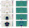 |
Fig. 1. Slow- and fast-wave evolution in a vertical cutting plane through the 3D null spine. Spatial maps of slow- (left column) and fast- (right column) wave amplitudes (in terms of their associated wave energy fluxes, i.e., |


To better appreciate the difference in the wave-mode evolution, we compare the results with our earlier rotational driver with the current vertical driver setup. Figure 2 displays the scaled velocity perturbations associated with all three MHD waves, that is, with the slow wave, fast wave, and Alfvén wave in the left, middle, and right column, respectively, for the rotational driver (top row) and vertical driver (bottom row). With the rotational driver, most wave energy flux ended up in Alfvén waves, with a substantial fraction of energy flux in the slow wave. Fast waves are generated by the mode conversion of slow waves at the Alfvén-acoustic equipartition layers. Fast waves reflect and are trapped below the transition region, with almost no accumulation of fast waves near the null point (Yadav et al. 2022). In sharp contrast, for vertical driving, most flux is in the slow mode, with negligible flux in the Alfvén mode.
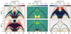 |
Fig. 2. Comparison of the wave transformations between rotational and p-mode drivers. We show maps of slow waves (left column), fast waves (middle column), and Alfvén waves (right column) at one instant close to the end of our time series (i.e., ∼47 min for both simulations). The top panel shows the distribution when applying a rotational driver at the bottom boundary, and the bottom panel corresponds to vertical velocity driving. |
To visualize how the waves behave over the entire 3D region, we show the velocity perturbations in Fig. 3 in a 3D cross-sectional view of the domain. The upper panel corresponds to rotational driving, and the bottom row corresponds to vertical driving. The results are shown for one instant; a movie for the time evolution during the full-time series is available as supplementary material. A few results are immediately clear from this figure. The bottom row confirms that the slow mode is dominant while they excite waves of modest amplitudes in the fast and Alfvén families with the vertical velocity driver. There is negligible power in the fast mode in both cases. Most of the wave power is in the Alfvén mode in the case of the rotational driver, while there is not much Alfvén power in the domain when a vertical velocity driver is used.
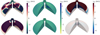 |
Fig. 3. Velocity perturbations of slow, fast, and Alfvén modes. We show a 3D cross-sectional view at the end of our time series for slow (left), fast (middle), and Alfvén wave (right). The top and bottom rows correspond to rotational and vertical driving, respectively. The movie of the wave propagation is available online. |
Finally, we can use the decomposition to quantify the energy fluxes of the three MHD wave types along the three previously discussed flux surfaces using the method described in our earlier work. We only analyze the vertical driver case here, and the rotational counterpart is found in Yadav et al. (2022). Figure 4 compares the wave energy flux distribution among three MHD wave modes (left column) and among acoustic and magnetic components (right column) for three selected constant flux surfaces (the surfaces are those shown in our current Fig. 2). The left column clearly shows that most of the wave energy flux is associated with the slow magnetoacoustic wave, which is expected because our wave driver is in vertical velocity and is almost parallel to the background magnetic field in the layers close to the solar surface. On the green surface, the driver directly acts near the leftmost s = 0 region. There, the velocity perturbation is hence a longitudinal velocity vector corresponding to slow magnetoacoustic waves in low plasma beta regions. These are indicated by the region in between the two vertical yellow lines in the top two rows of this figure. Because the blue surface passes very close to the null point, the signatures of wave-mode conversion are clear there in the obvious transformations that occur at s ≈ 3 Mm. The energy flux available in fast waves increases rapidly, while energy flux available in slow waves decreases. For all surfaces, the energy flux associated with Alfvén waves remains negligible compared to that in the other two wave modes. Similarly, in the right column, most of the energy flux is acoustic flux, which is expected because slow waves are acoustic in nature in the low plasma beta regions. Again, in the case of the blue surface, the magnetic component of energy flux increases and the acoustic component of energy flux decreases close to the null point, which can be attributed to mode conversion.
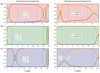 |
Fig. 4. Energy flux comparisons for the three selected flux surfaces. The surfaces are indicated as background colors: red (top row), green (middle row), and blue (bottom row). Left column: Energy fluxes associated with slow, fast, and Alfvén waves. Right column: Acoustic and magnetic fluxes. The vertical lines represent the locations of the Alfvén-acoustic equipartition layer (yellow) and the transition region (turquoise). |
3.2. Current accumulation at the null point
Coronal null points are crucial from an energy perspective because in these locations, the Alfvén speed is zero, and waves traveling with this speed can no longer propagate. Previous studies have shown that fast waves approaching the null point may wrap around it and lead to an increase in current density at the null point (McLaughlin & Hood 2004; McIntosh et al. 2011). To verify this current accumulation in our numerical setup, we calculated the time-averaged (over three wave periods) current density shown in Fig. 5 for a vertical plane y = 0, where the field lines are indicated in red. As expected, this vertical driver now indeed leads to strong current accumulation around the null point, which was absent in the case of the spiral driver (see Fig. 9 of Yadav et al. 2022 for comparison). We did not include resistivity to allow a fair comparison to our previous setup used in Yadav et al. (2022). The current buildup around the magnetic null point suggests the potential for Joule dissipation and subsequent heating. The current accumulation near the region in which the driver is located is mostly due to fast-wave reflection. The current accumulation at ±10 Mm, however, is a boundary condition effect because the fast waves generated near the null point travel and are reflected at the surface.
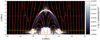 |
Fig. 5. Spatial map of the magnitude of current (time-averaged over three wave periods) shown for a y = 0 slice through the domain. |
Because the periodic wave driver causes the current to accumulate at the null point, we further studied the potential heating signature and modulation in the thermal emission profile. We integrated the square of the absolute value of current in the surrounding region of the null point and plot its variation with time in Fig. 6. This quantity is directly proportional to Ohmic dissipation and gives an indirect estimate of the temporal variation of plasma heating around the null point. These periodic modulations in the magnitude of current around the null might result in periodic variations in plasma temperatures. They can be associated with quasi-periodic pulsations (QPPs) in solar and stellar flares or in similar periodic energetic events. Here, it is important to note that the oscillation frequency of the current magnitude is twice the frequency of the input wave driver. The possible relation between p-modes and the periodicity of QPPs has been of great interest in the past few decades. There is observational evidence that the energy of three-minute oscillations in the active regions is significantly increased before the occurrence of the solar flare, and the associated light curves show pronounced variations with similar periods and their higher harmonics (Sych et al. 2009; Hayes et al. 2019; Kolotkov et al. 2015).
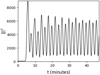 |
Fig. 6. Time evolution of the square of the current density in the region surrounding the null point. |
4. Conclusions
Magnetic null points are one manifestation of the complex topology of magnetic fields in the solar corona. In these locations in space, the magnetic field vanishes. They are regarded as proxies for magnetic reconnection sites and current dissipation. Their inherently 3D nature means that it is difficult to investigate the process of magnetic reconnection and current dissipation around magnetic nulls using observations from one vantage point (Reep & Knizhnik 2019; Cheng et al. 2023). Statistically, eruptive events are encountered more frequently in active regions with null points than in regions without null points (Barnes 2007). Thus, it is crucial to investigate MHD dynamics using dedicated simulations to unravel the physical mechanisms of various processes associated with coronal magnetic null points. To this end, we used our open-source MPI-AMRVAC code to perform simulations of the solar atmosphere ranging from the photosphere to the solar corona, such that the atmosphere is gravitationally stratified and the magnetic field has a complex topology representative of a coronal null point.
In observations, the periodicity of MHD waves is often shown to be linked with the periodicity of quasi-periodic oscillations detected in intensity enhancements at the null point (Foullon et al. 2005; Van Doorsselaere et al. 2011; Su et al. 2012). Nakariakov & Verwichte (2005) attributed it to the influence of external evanescent or leaking parts of the wave oscillation that can reach the null point. Using MHD simulations, Chen & Priest (2006) demonstrated that five-minute solar p-mode oscillations can also lead to periodically triggered reconnection and thus transfer their periodicities in QPPs. Murray et al. (2009), in contrast, investigated the emergence of a buoyant flux tube in a stratified atmosphere permeated by a unipolar magnetic field and reported that periodic reconnection takes place as the system searches for equilibrium. More recently, Li et al. (2023) showed the formation of a null point as a result of the process of flux emergence and investigated the associated reconnecting plasmoid chains and the occurrence of multithermal jets. Thurgood et al. (2017) demonstrated the interconnected nature of magnetic reconnection and MHD waves. They showed that magnetic reconnection at realistic 3D magnetic null points naturally proceeds in an oscillatory fashion and produces MHD waves. Various other mechanisms have been proposed in the literature that can explain the observed periodicity of intensity enhancements at null points (e.g., see the review by McLaughlin et al. 2018). However, there is currently no consensus in the solar physics community on a physical mechanism that can unambiguously explain all quasi-periodic intensity variations at null points. Because their periodicity does approximately coincide with that of the MHD waves that are abundantly detected in the solar corona, we examined the interaction of acoustic p-modes with a coronal null topology and investigated the wave transformations in detail.
To replicate the effect of global p-modes, we employed a vertical wave driver at the bottom boundary acting in the central region around the null spine. Because the background magnetic field is mostly vertical in the wave excitation region, most vertical velocity perturbation travels in slow waves. These slow waves undergo secondary wave mode conversion at the Alfvén acoustic equipartition layer, generating a fast mode that leads to current accumulation at the null point. Fast modes generated at the first equipartition layer are reflected from the sharp density gradients at the transition region and remain trapped below it. These results indirectly indicate that the fast waves that are often observed at the null point have a different source of excitation from the mode conversion at the Alfvén acoustic equipartition layer below the transition layer. We showed that the fast modes are focused at the null point and lead to localized currents. They are not generated below the transition region, however, but in the surrounding surface of the null point where another Alfvén acoustic equipartition condition exists. Moreover, the periodicity of resistive dissipation is compatible with the second harmonic of wave driving, as has often been observed. Thus, we conjecture that although the periodicity of the quasi-periodic intensity enhancement at the null point covers a vast range, it might be determined by the dominant wave period excited at the solar surface. It is worthwhile to mention here that the current accumulation near the region in which the driver is located is mostly due to fast-wave reflection. In contrast, the current accumulation at ±10 Mm is a boundary condition effect because the fast waves generated near the null point travel and are reflected at the surface.
Moreover, QPPs are often shown to exhibit a periodicity that is consistent with higher harmonics of MHD waves (McLaughlin et al. 2009; Threlfall et al. 2012). Analyzing the observations in X-ray, microwave, and extreme ultraviolet bands for the decay phase of an X-class solar flare, Kupriyanova et al. (2019) reported that the second harmonic of the slow magnetoacoustic mode is the most likely explanation for the observed periods of QPPs. However, they were unable to verify the possible mechanism of the intensity enhancements at the periodicity corresponding to the second harmonic. With the model presented here, we clearly demonstrated that the mode conversion of p-modes may lead to the generation of fast modes surrounding the null point. We expect that the current fluctuations would produce intensity enhancement at the second harmonic by joule dissipation, which needs to be confirmed by follow-up resistive MHD simulations that can be used for synthetic views. One limitation of the current model is that we dealt only with the linear regime of the MHD waves so that we could directly compare our results with those from our previous study (Yadav et al. 2022). However, as a future step, it would be interesting to see how the results obtained here are modified in a nonlinear regime, in which we could also include the nonideal terms in our setup, such as thermal conduction and radiative losses.
Movie
Movie 1 associated with Fig. 3 (movie(2)) Access Supplementary Material
Acknowledgments
NY and RK are supported by Internal funds KU Leuven, project C14/19/089 TRACESpace. RK further received funding from the European Research Council (ERC) under the European Union’s Horizon 2020 research and innovation programme (grant agreement no. 833251 PROMINENT ERC-ADG 2018), and FWO grant G0B4521N. NY acknowledges the support provided by DST INSPIRE Fellowship under grant number DST/INSPIRE/04/2021/001207.
References
- Bagashvili, S. R., Shergelashvili, B. M., Japaridze, D. R., et al. 2018, ApJ, 855, L21 [NASA ADS] [CrossRef] [Google Scholar]
- Barnes, G. 2007, ApJ, 670, L53 [Google Scholar]
- Brandt, P. N., Scharmer, G. B., Ferguson, S., et al. 1988, Nature, 335, 238 [NASA ADS] [CrossRef] [Google Scholar]
- Cally, P. S. 2005, MNRAS, 358, 353 [Google Scholar]
- Cally, P. S. 2006, Philos. Trans. R. Soc. London Ser. A, 364, 333 [Google Scholar]
- Cally, P. S., & Goossens, M. 2008, Sol. Phys., 251, 251 [Google Scholar]
- Chen, P. F., & Priest, E. R. 2006, Sol. Phys., 238, 313 [Google Scholar]
- Cheng, X., Priest, E. R., Li, H. T., et al. 2023, Nat. Commun., 14, 2107 [NASA ADS] [CrossRef] [Google Scholar]
- Cranmer, S. R., & van Ballegooijen, A. A. 2005, ApJS, 156, 265 [Google Scholar]
- Felipe, T. 2012, ApJ, 758, 96 [Google Scholar]
- Foullon, C., Verwichte, E., Nakariakov, V. M., & Fletcher, L. 2005, A&A, 440, L59 [NASA ADS] [CrossRef] [EDP Sciences] [Google Scholar]
- Galsgaard, K., Priest, E. R., & Titov, V. S. 2003, J. Geophys. Res. (Space Phys.), 108, 1042 [NASA ADS] [CrossRef] [Google Scholar]
- Hayes, L. A., Gallagher, P. T., Dennis, B. R., et al. 2019, ApJ, 875, 33 [Google Scholar]
- Joshi, R., Chandra, R., Schmieder, B., et al. 2020, A&A, 639, A22 [NASA ADS] [CrossRef] [EDP Sciences] [Google Scholar]
- Keppens, R., Teunissen, J., Xia, C., & Porth, O. 2021, Comput. Math. Appl., 81, 316 [Google Scholar]
- Keppens, R., Popescu Braileanu, B., Zhou, Y., et al. 2023, A&A, 673, A66 [NASA ADS] [CrossRef] [EDP Sciences] [Google Scholar]
- Khomenko, E., & Cally, P. S. 2012, ApJ, 746, 68 [Google Scholar]
- Khomenko, E., & Collados, M. 2006, ApJ, 653, 739 [Google Scholar]
- Kolotkov, D. Y., Nakariakov, V. M., Kupriyanova, E. G., Ratcliffe, H., & Shibasaki, K. 2015, A&A, 574, A53 [NASA ADS] [CrossRef] [EDP Sciences] [Google Scholar]
- Kumar, P., Nakariakov, V. M., & Cho, K.-S. 2016, ApJ, 822, 7 [Google Scholar]
- Kumar, P., Nakariakov, V. M., & Cho, K.-S. 2017, ApJ, 844, 149 [Google Scholar]
- Kupriyanova, E. G., Kashapova, L. K., Van Doorsselaere, T., et al. 2019, MNRAS, 483, 5499 [NASA ADS] [CrossRef] [Google Scholar]
- Li, X., Keppens, R., & Zhou, Y. 2023, ApJ, 947, L17 [NASA ADS] [CrossRef] [Google Scholar]
- Liu, W., Title, A. M., Zhao, J., et al. 2011, ApJ, 736, L13 [NASA ADS] [CrossRef] [Google Scholar]
- Liu, W., Ofman, L., Nitta, N. V., et al. 2012, ApJ, 753, 52 [NASA ADS] [CrossRef] [Google Scholar]
- McIntosh, S. W., de Pontieu, B., Carlsson, M., et al. 2011, Nature, 475, 477 [Google Scholar]
- McLaughlin, J. A., & Hood, A. W. 2004, A&A, 420, 1129 [NASA ADS] [CrossRef] [EDP Sciences] [Google Scholar]
- McLaughlin, J. A., & Hood, A. W. 2006, A&A, 459, 641 [NASA ADS] [CrossRef] [EDP Sciences] [Google Scholar]
- McLaughlin, J. A., De Moortel, I., Hood, A. W., & Brady, C. S. 2009, A&A, 493, 227 [NASA ADS] [CrossRef] [EDP Sciences] [Google Scholar]
- McLaughlin, J. A., Nakariakov, V. M., Dominique, M., Jelínek, P., & Takasao, S. 2018, Space Sci. Rev., 214, 45 [Google Scholar]
- Moradi, H., & Cally, P. S. 2013, J. Phys. Conf. Ser., 440, 012047 [NASA ADS] [CrossRef] [Google Scholar]
- Moreno-Insertis, F., Galsgaard, K., & Ugarte-Urra, I. 2008, ApJ, 673, L211 [Google Scholar]
- Morton, R. J., Tomczyk, S., & Pinto, R. 2015, Nat. Commun., 6, 7813 [Google Scholar]
- Murray, M. J., van Driel-Gesztelyi, L., & Baker, D. 2009, A&A, 494, 329 [NASA ADS] [CrossRef] [EDP Sciences] [Google Scholar]
- Nakariakov, V. M., & Melnikov, V. F. 2009, Space Sci. Rev., 149, 119 [Google Scholar]
- Nakariakov, V. M., & Verwichte, E. 2005, Liv. Rev. Sol. Phys., 2, 3 [Google Scholar]
- Popescu Braileanu, B., & Keppens, R. 2021, A&A, 653, A131 [NASA ADS] [CrossRef] [EDP Sciences] [Google Scholar]
- Priest, E. R., & Forbes, T. G. 2002, A&ARv, 10, 313 [Google Scholar]
- Reep, J. W., & Knizhnik, K. J. 2019, ApJ, 874, 157 [NASA ADS] [CrossRef] [Google Scholar]
- Santamaria, I. C., Khomenko, E., & Collados, M. 2015, A&A, 577, A70 [NASA ADS] [CrossRef] [EDP Sciences] [Google Scholar]
- Santamaria, I. C., Khomenko, E., Collados, M., & de Vicente, A. 2017, A&A, 602, A43 [NASA ADS] [CrossRef] [EDP Sciences] [Google Scholar]
- Schmieder, B. 2022, Front. Astron. Space Sci., 9, 820183 [NASA ADS] [CrossRef] [Google Scholar]
- Schmieder, B., Guo, Y., Moreno-Insertis, F., et al. 2013, A&A, 559, A1 [NASA ADS] [CrossRef] [EDP Sciences] [Google Scholar]
- Shibata, K., Ishido, Y., Acton, L. W., et al. 1992, PASJ, 44, L173 [Google Scholar]
- Spruit, H. C. 1981, A&A, 98, 155 [NASA ADS] [Google Scholar]
- Stangalini, M., Consolini, G., Berrilli, F., De Michelis, P., & Tozzi, R. 2014, A&A, 569, A102 [NASA ADS] [CrossRef] [EDP Sciences] [Google Scholar]
- Su, J. T., Shen, Y. D., Liu, Y., Liu, Y., & Mao, X. J. 2012, ApJ, 755, 113 [NASA ADS] [CrossRef] [Google Scholar]
- Sych, R., Nakariakov, V. M., Karlicky, M., & Anfinogentov, S. 2009, A&A, 505, 791 [NASA ADS] [CrossRef] [EDP Sciences] [Google Scholar]
- Tarr, L. A., & Linton, M. 2019, ApJ, 879, 127 [NASA ADS] [CrossRef] [Google Scholar]
- Tarr, L. A., Linton, M., & Leake, J. 2017, ApJ, 837, 94 [NASA ADS] [CrossRef] [Google Scholar]
- Threlfall, J., Parnell, C. E., De Moortel, I., McClements, K. G., & Arber, T. D. 2012, A&A, 544, A24 [NASA ADS] [CrossRef] [EDP Sciences] [Google Scholar]
- Thurgood, J. O., Pontin, D. I., & McLaughlin, J. A. 2017, ApJ, 844, 2 [Google Scholar]
- Van Doorsselaere, T., De Groof, A., Zender, J., Berghmans, D., & Goossens, M. 2011, ApJ, 740, 90 [NASA ADS] [CrossRef] [Google Scholar]
- Volkmer, R., Kneer, F., & Bendlin, C. 1995, A&A, 304, L1 [NASA ADS] [Google Scholar]
- Wedemeyer-Böhm, S., Scullion, E., Steiner, O., et al. 2012, Nature, 486, 505 [Google Scholar]
- Xia, C., Teunissen, J., El Mellah, I., Chané, E., & Keppens, R. 2018, ApJS, 234, 30 [Google Scholar]
- Yadav, N., Cameron, R. H., & Solanki, S. K. 2021, A&A, 652, A43 [NASA ADS] [CrossRef] [EDP Sciences] [Google Scholar]
- Yadav, N., Keppens, R., & Popescu Braileanu, B. 2022, A&A, 660, A21 [NASA ADS] [CrossRef] [EDP Sciences] [Google Scholar]
All Figures
|
Fig. 1. Slow- and fast-wave evolution in a vertical cutting plane through the 3D null spine. Spatial maps of slow- (left column) and fast- (right column) wave amplitudes (in terms of their associated wave energy fluxes, i.e., |
| In the text | |
|
Fig. 2. Comparison of the wave transformations between rotational and p-mode drivers. We show maps of slow waves (left column), fast waves (middle column), and Alfvén waves (right column) at one instant close to the end of our time series (i.e., ∼47 min for both simulations). The top panel shows the distribution when applying a rotational driver at the bottom boundary, and the bottom panel corresponds to vertical velocity driving. |
| In the text | |
|
Fig. 3. Velocity perturbations of slow, fast, and Alfvén modes. We show a 3D cross-sectional view at the end of our time series for slow (left), fast (middle), and Alfvén wave (right). The top and bottom rows correspond to rotational and vertical driving, respectively. The movie of the wave propagation is available online. |
| In the text | |
|
Fig. 4. Energy flux comparisons for the three selected flux surfaces. The surfaces are indicated as background colors: red (top row), green (middle row), and blue (bottom row). Left column: Energy fluxes associated with slow, fast, and Alfvén waves. Right column: Acoustic and magnetic fluxes. The vertical lines represent the locations of the Alfvén-acoustic equipartition layer (yellow) and the transition region (turquoise). |
| In the text | |
|
Fig. 5. Spatial map of the magnitude of current (time-averaged over three wave periods) shown for a y = 0 slice through the domain. |
| In the text | |
|
Fig. 6. Time evolution of the square of the current density in the region surrounding the null point. |
| In the text | |
Current usage metrics show cumulative count of Article Views (full-text article views including HTML views, PDF and ePub downloads, according to the available data) and Abstracts Views on Vision4Press platform.
Data correspond to usage on the plateform after 2015. The current usage metrics is available 48-96 hours after online publication and is updated daily on week days.
Initial download of the metrics may take a while.