| Issue |
A&A
Volume 681, January 2024
|
|
|---|---|---|
| Article Number | A102 | |
| Number of page(s) | 11 | |
| Section | Astronomical instrumentation | |
| DOI | https://doi.org/10.1051/0004-6361/202346902 | |
| Published online | 23 January 2024 | |
Eigenbases for a force-constrained position control of adaptive shell mirrors
1
ESO Headquarters Karl-Schwarzschild-Str. 2,
85748
Garching bei München,
Germany
e-mail: This email address is being protected from spambots. You need JavaScript enabled to view it.
2
Space ODT – Optical Deblurring Technologies Ltd,
Porto,
Portugal
Received:
15
May
2023
Accepted:
3
August
2023
Abstract
Context. The deployment of meter-scale (hitherto pre-focal) adaptive deformable mirrors finds some prominent examples in the leading ground-based visible to near-infrared facilities (e.g. the Very Large Telescope (VLT), the Large Binocular Telescope (LBT), or the Magellan Telescope) and is being adopted by several others (e.g. the Multiple Mirror Telescope (MMT) or Subaru). Furthermore, two out of the three giant segmented-mirror telescopes now under design will feature them. In all these cases, the proprietary technology is based on voice-coils and is limited in force, stroke, and velocity.
Aims. Because of the nature of their purpose, that is, adaptive wave-front correction, any kind of optimality relies on the control of a subset of principal wave-front components or eigenmodes, for short, a basis of functions in a mathematical sense. Here we provide algorithmic procedures for generating such eigenbases, also called Karhunen–Loève (KL) modes, that integrate force limitations in their definitions whilst maintaining standard orthonormality, statistical independence, and deformable mirror span.
Methods. The double-diagonalisation method was revisited to build KL modes ranked by the force applied on the actuators.
Results. We analysed this new KL basis for von Kármán turbulence statistics and present the fitting error and the distribution of positions and forces. We further illustrate their use in the case of the quaternary mirror control for the European Extremely Large Telescope, and we include the outer actuator minioning and force policy constraints.
Key words: instrumentation: adaptive optics / telescopes / methods: analytical
© The Authors 2024
 Open Access article, published by EDP Sciences, under the terms of the Creative Commons Attribution License (https://creativecommons.org/licenses/by/4.0), which permits unrestricted use, distribution, and reproduction in any medium, provided the original work is properly cited.
This article is published in open access under the Subscribe to Open model. This email address is being protected from spambots. You need JavaScript enabled to view it. to support open access publication.
1 Introduction
Adaptive shell (hitherto pre-focal) deformable mirrors (DM; Salinari et al. 1994) bring adaptive optics (AO) into the core of the optical path of a telescope. Unlike classical post-focal instrument-proprietary AO, these adaptive telescopes promise to reduce the number of reflecting surfaces leading to improve near-IR (NIR) observations, larger corrected fields, more compact optical designs, and so on.
Notable examples are the deformable secondary at the Multiple Mirror Telescope (MMT) Brusa et al. (2003), the Very Large Telescope Adaptive Optics Facility (VLT-AOF) Arsenault et al. (2006), and the adaptive secondaries of the Large Binocular Telescope (LBT) Riccardi et al. (2010) and Magellan telescopes Close et al. (2010), all based on the Microgate technology. Future giant segmented-mirror telescopes such as the European Extremely Large Telescope (ELT) and the Giant Magellan Telescope (GMT) will feature adaptive secondaries based on voice-coil technology. As we show below, the developments made here will therefore cater to any of these systems.
The shells surface is deformed by controlling actuator positions recurring to an inner closed loop at frame rates that are orders of magnitude higher than typical AO frame-rates, using position sensors (e.g. capacitive sensors). These dynamic details are unimportant for the analysis that ensues because from an AO point of view, they occur much beyond the bandwidths relevant for our analysis. However, the budget of local forces applied to the location of the actuators along the z-axis orthogonal to the surface is limited to a few Newton. Other limitations in terms of stroke and velocity also apply, but they fall outside of the modal basis optimisation that we intend to outline here because i) they concern amplitude, which cannot be encoded in a basis, and ii) they concern velocity, which is a time dimension parallel to the space dimension covered here.
Classical DMs are controlled by minimising one quantity (either voltages or currents) that directly drive the local displacement of the DM actuators. Unlike the latter, the fast inner position-control loop in adaptive shells means that their response is not passive, but active. The commands sent to the DM thus achieve a different nature: they become z position setpoints that are kept in place by the inner control loop. Despite this, the local deformations (whether passive or active) can still be represented by a steady-state influence function that describes the bi-dimensional optical-path-difference (OPD) deformation in response to a unitary command.
We present an evolution of the double-diagonalization method (Gendron 1995) that is employed to build a modal basis for wave-front (WF) reconstruction in AO. Our purpose is to revisit the generation of control bases that conserve key properties. The first property is that the bases correspond to the principal components of the atmospheric turbulence. The second property is that they are statistically independent. The third property is that they are orthonormal in phase space with respect to the primary aperture. The fourth property is that they are fully defined in the space spanned by the deformable mirror. To these properties, the control of thin adaptive shells adds constraints in terms of force, which we factor in the generation of the control basis itself whilst keeping the above properties intact.
Without loss of generality, the presentation that follows is illustrated for (and motivated by) the case of the European Extremely Large Telescope (ELT) pre-focal quaternary deformable mirror (the M4) Vernet et al. (2019, ?). We consider an interface to the DM where the command vector is the vector of actuator mechanical position setpoints.
To do this, we revisit the Karhunen–Loeve (KL) modal basis generation through double-diagonalisation in Sect. 3 and then expand it to force minimisation in Sect. 4.
2 KL modal expansion
The KL modal expansion of space- and time-indexed processes is one of the most frequently used statistical techniques for the feature extraction of continuous stochastic processes. In its discrete formulation, it is simply empirical orthogonal function (EOF) analysis or principal component analysis (PCA) Fontanella & Ippoliti (2012). Hence, both KL expansion and EOF are useful for efficiently reducing the dimension of large degree-of-freedom data-sets. In its simplest description, it is the solution of the covariance eigenvalue equation.
We outline the steps for synthesising (but also to analysing) a basis set of functions (or modes) to describe the wavefront on a given telescope pupil, over which the modal expansion writes
 (1)
(1)
where b⊤ is the transpose vector of modal coefficients, and ℬ(r) are the basis functions (modes) indexed by the bi-dimensional variable r. It is useful to define an inner product between two bi-dimensional functions f1(r) and f2(r),
 (2)
(2)
where the binary aperture function Ω(r) is zero-one valued for points outside or inside the pupil, respectively. The KL modes are eigenfunctions and therefore respect two properties: the first one is the orthonormality with respect to Ω(r)
 (3)
(3)
and the second one is the statistical independence
 (4)
(4)
where δij is the Kronecker symbol, and 〈⋅〉 represents the ensemble average. From these equations, we obtain the two-dimensional KL integral equation
 (5)
(5)
Eigendecomposition of 〈ϕ(r)ϕ(r)〉
The KL modes can instead be computed numerically for any pupil type, form, or shape, with or without central obstruction. In this case, we compute the eigenvectors of the phase covariance function whose columns express the KL modes on the chosen underlying basis.
Adopting a discrete, point-wise description of the phase (also called zonal expansion), we determine the phase covariance matrix Cϕ = 〈ϕ(r)ϕ(r)〉 = 〈ϕϕ⊤〉 by summing over all the layers that were sampled by the values of the covariance function Cl(ρ) at i, j ∊ Ω. We compute  , which is shorthand notation for a square matrix of the distances between all the intercepts within the considered aperture (whose shape can be any desired shape),
![Mathematical equation: ${{\bf{C}}_\phi }[i,j] = \sum\limits_l {{C_l}} \left( {\rho = \left| {{{\bf{r}}_i} - {{\bf{r}}_j}} \right|} \right)\quad \forall \quad {{\bf{r}}_i},{{\bf{r}}_j} \in {{\rm{\Omega }}_l},$](/articles/aa/full_html/2024/01/aa46902-23/aa46902-23-eq7.png) (6)
(6)
where
 (7)
(7)
if ρ>0, and
 (8)
(8)
otherwise Conan et al. (2000); Sasiela (1994). L0 is the outer scale of turbulence, here assumed constant over all layers, r0(l) is Fried’s parameter, Γ(⋅) is the gamma function, and K5/6(⋅) is a modified Bessel function of the third order.
An example is provided in Fig. 1. The figure depicts commonly accepted KL modes such as slightly bent tilt modes and a family of Zernike-resembling modes computed from the eigen-decomposition of the piston-removed spatial phase covariance matrix shown in Fig. 2.
Alternative methods that care to provide an orthonormal basis on arbitrary pupil shapes use for example Gram–Schmidt minimisation (Upton & Ellerbroek 2004), but they fall short of a basis retaining all the key features for AO control (listed in the introduction).
Furthermore, it is convenient to express the basis functions within the space spanned by the deformable-mirror (DM) influence functions (IFs). This step is necessary to build a basis that is relevant for AO control. It leads not to one, but to two eigenvalue-determination problems, as is explained next.
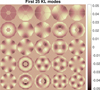 |
Fig. 1 Face-on representation of the first 25 KL modes obtained from the eigenmodes of the piston-removed phase covariance matrix in Fig. 2. The first mode corresponds to a numerical leftover of the piston. |
3 Original double-diagonalisation method
The developments covered here were first presented in Gendron (1995) with the purpose of realising the so-called optimal modal gain integrator (OMGI), a technique whereby a set of (spatial) control modes are optimally weighted to obtain the lowest wave-front residual. Some mathematical aspects presented in Lai et al. (2000) were used as the starting point of our work. The method is called double-diagonalisation because it requires two steps involving the calculation of eigenmodes of some quantity in some space.
The concept behind the generation of one such KL basis is the following: the generation of the principal components of the atmosphere (stochastic process) is expressed as a linear combination of the DM principal components (geometric steady-state modes).
Mathematically, we seek the basis B of modes that respects
 (9)
(9)
with C is a statistical covariance matrix (from turbulence), and Δ a geometric cross-product matrix of DM IFs (sometimes also called geometric covariance matrix) to ensure orthonormality between the modes. Both are symmetric and positive definite.
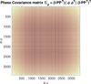 |
Fig. 2 Piston-removed zonal spatial covariance matrix using lexicographic indexing for a pupil shown in Fig. 1. The equation in the title corresponds to the development of 〈‖ϕ − ϕP‖2〉, where the piston mode is ϕP = P ⋅ P⊤ ⋅ ϕ. |
3.1 Definition of DM related variables
The vector space spanned by the DM is given by the steady-state IFs representing the most complete basis of the DM. The OPD is the shape of the WF after reflection by the deformable mirror. Any valid OPD deformation of the DM can be decomposed uniquely in the IF space,
 (10)
(10)
where pi is the ith actuator command setpoints, and hi is the ith bi-dimensional influence function.
From now on and for compactness, we write the equations in the form of matrix operations whenever possible (the dot operator representing the matrix multiplication), and when we define a matrix, we append the explicit dimensions as follows: M[dima, dimb]. Hence the matrix representation of Eq. (10) becomes
 (11)
(11)
where ϕ[np] is the vector of the np valid OPD numerical points within the pupil, and p[nact] is the vector of the actuator positions (throughout this paper, the position of an actuator denotes the mechanical displacement of the shell surface in the centre of the actuator along the z-axis). We consider in the nact set all actuators, regardless of whether within or outside of the pupil. H[np, nact] is the matrix that collects the IFs as vectors on the valid pupil points in its columns. The two variables ϕ and p are expressed in meters.
We define for later use a handy geometric IFs cross-product matrix Δ, which also appears in Eq. (9) and is given by
 (12)
(12)
In the classical method, it is common practice to select a number of valid actuators nsel defined by some reasonable criterion. In this case, the influence matrix is limited to the selected actuators (H[np, nsel]), and Δ[nsel, nsel] is assumed to be invertible.
To any vector p corresponds a vector of forces f[nact] that is expressed as a function of a stiffness matrix K[nact, nact] (expressed in newton-meter),
 (13)
(13)
In the case of M4, the matrix K is a block diagonal matrix in which each block is equal to the stiffness matrix for a shell (all six shells are carbon copies of each other). This is common knowledge, and the method developed here is general enough to cover cases of non-segmented shells.
The least-squares solution for the best fit in terms of DM positions pfit to an input OPD ϕ can be written in a general form with the Tikhonov regularisation matrix V:
 (14)
(14)
In the classical method of a least-squares fit with actuator selection, in Eq. (14), V = 0, and Δ is invertible.
3.2 Specific modes and seed basis
The first step in the definition of a useful modal basis for control in AO is to define specific modes (SpM) that explicitly appear in the basis. The simplest example is piston and tip-tilt modes, but it can be any modes that are to either be controlled or discarded from the reconstruction.
We define nspm, the number of SpMs, and ϕspm[np, nspm], the exact pupil-bounded OPD shape to fit. We use the notation of Ferreira et al. (2018) to write the best fit (in positions space) τ[nsel, nspm] to the OPD of SpMs ϕspm,
 (15)
(15)
This defines the SpM. Its complementary space H⊥ on which we build the orthonormal seed basis SB[nsel, nsel − nspm] is defined by subtracting the projection of each IF on the SpM,
 (16)
(16)
which can be expressed in terms of a generator G[nsel, nsel] of modified IFs,
 (17)
(17)
where G is given by Ferreira et al. (2018)
 (18)
(18)
and is readily obtained by plugging Eq. (15) into Eq. (16) and further developing terms. The seed basis is defined by
 (19)
(19)
where D and Λ are the eigenvectors and diagonal matrix, respectively, of the eigenvalues of the cross product of H⊥,
 (20)
(20)
where we use some abuse of notation svd(⋅) to represent the singular-value decomposition (SVD), which formally provides three matrices, the product of which is the one shown.
We note that from Eq. (20), D is a collection of eigenvectors expressed in components of G (modified IFs). Hence, to obtain SB, expressed in actuator space (original IFs), a change of basis from G to actuators is performed by multiplication by G in front of Eq. (19). Then, using the definition and unitary nature of D, it is straightforward to show that SB is an orthonormal basis and therefore verifies (H.SB)⊤.H.SB = I. We caution that this way of computing DM eigenmodes uses a particular property (invertibility) of the cross product Δ and will no longer hold when force minimisation is considered. This is explained in Sect. 4.2.
3.3 KL modes
The two properties of KLs we are interested in are statistical independence for turbulence correction and orthonormality in OPD space. We define the covariance matrix Cp as the covariance of the best-fit positions (Eq. (14) with V = 0) for atmospheric turbulence (Kolmogorov or von Kármán) statistics,
 (21)
(21)
The ensemble average is done over independent realisations of turbulence phase ϕ. The matrix Cp has been derived in Gendron (1995) and Lai et al. (2000), and we rewrite the derivation in a slightly different way in Appendix A. The different writing supports the generalisation to a force-optimised basis.
The KL modes are the eigenmodes A of Cp expressed in the seed basis in order to satisfy the two properties. The matrix KL[nact, nact − nspm] represents the actuators position setpoints encapsulating the KL shapes,
 (22)
(22)
where A is obtained from the SVD of Cp after a change of basis to SB,
 (23)
(23)
Working versions used in classical double-diagonalisation are publicly available in Matlab and IDL (and maybe other codes). An example is 00MA0 (Conan & Correia 2014).
The diagonal matrix S gives the spectrum, root mean square (RMS) of the OPD, of the turbulent phase projected on the KLs, and we have
 (24)
(24)
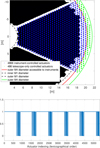 |
Fig. 3 Top: ELT quaternary mirror (M4) geometry projected on the primary mirror (M1) coordinates and overlaid on the M1 pupil. Enlargement of one of the six independent sectors. Bottom: 5352 actuators column-wise indexed by lexicographical order. 1 indexes the blue dots (inner actuators), and 0 indexes the green dots (outer actuator). |
Complete basis
The complete basis is the concatenation of the SpM and the KL modes,
![Mathematical equation: ${\bf{B}} = [\tau \mid {\bf{KL}}].$](/articles/aa/full_html/2024/01/aa46902-23/aa46902-23-eq26.png) (25)
(25)
This matrix is commonly called in adaptive-optics jargon the modes-to-commands (M2C) matrix and it is all that is needed to perform AO modal control.
4 Double diagonalisation and force minimisation
In the preceding section, only the selected actuators nsel inside or very near the pupil were considered. In this case, Δ is invertible, and an orthonormal basis can always be found. In most of the AO systems, this is sufficient to define the command of the DM (an extrapolation at border actuators is sometimes applied).
For adaptive shell mirrors, the situation is different, and the DM with its actuator grid may be significantly larger than the pupil. For example, the ELT M4 presents an overall shell size of 2.40 m, while the optical pupil (for the centre of the field) has a size of 2.25 m. The diameter is 7% larger and represents about three rings of actuators (see Fig. 3).
In the particular case of M4, we need to control outer actuators with little or no influence on the phase in the pupil, and this despite the extrapolation imposed on the outermost actuators that follows from the classical methods. We consider now H[np, nact] defined for all actuators. Concretely, this means that Δ is no longer invertible (because it is ill conditioned), and hence, non-independent sets of modes can be obtained. Some computations such as inversions become pseudo-inversions, and diagonalisations involve the selection of valid eigenvectors. As for the method in this section, we always ensured that we sought an orthonormal basis (for the SpMs, the seed basis, or the KLs), not only to satisfy the original properties, but also as a guarantee that the resulting bases are independent.
For instance, for a basis B expressed in positions space, we define the orthonormality criterion CO as
 (26)
(26)
which we consider to be satisfied when it is of the order of the expected computer precision. A similar criterion is applied to check the diagonality of the statistical covariance matrix.
The concept of the method that follows is to compute the SpMs, seed basis, and KLs in force space (instead of position). However, we found that SpMs such as often-cases tilt modes appear associated with the lowest values of the stiffness matrix. In other words, low-order modes (or equivalently, low spatial-frequency modes) require the least force (lower by orders of magnitude when compared to higher-order modes). In the implementations made leading to the results of this paper, we found that expressing the basis in terms of force setpoints leads to numerical instabilities when projecting on low-order SpMs (e.g. tip and tilt). For this reason, we proceeded in three steps: the first step consists of finding the best OPD fit (expressed in positions setpoints) to SpMs by weighted least-squares projection on the space spanned by the DM IFs. The second step is determining the seed basis by diagonalisation in force-like space of the sub-space orthogonal to the SpMs. Then, express the resulting seed basis in position space. The third step is computing the KL basis as in the classical method (in position space), but with an adaptation to take the ill-conditioned Δ into account.
4.1 Specific modes: WF fitting with force regularisation
One natural way to determine the SpMs is to compute the positions using a regression with Tikhonov regularisation using the forces as a penalty term. We used Eq. (14) with Γ ≠ 0 and proportional to the stiffness matrix K,
 (27)
(27)
This is equivalent to minimising
 (28)
(28)
The solution minimises the fitting error while keeping the forces sufficiently low. α is the only parameter that is tuned. All actuators are considered valid. We can rewrite Eq. (15) and express τα, the best fit of the SpMs minimising forces, as
 (29)
(29)
where α needs to be adjusted until the two error sources in Eq. (28) reach acceptable values. Typical values in the case of M4 are α = 10−15 for low-order modes (piston, tip-tilt, differential piston modes, etc.) and must be adapted case by case. We suggest in any case to make a sanity check of the positions and forces obtained. We also realised that cropping the influence function to save memory may affect the optimum α values significantly.
4.2 First diagonalisation: A seed basis from expressing OPD as a function of force
The classical way of computing the first diagonalisation is equivalent to analysing OPD as a function of DM actuator position setpoints. The DM eigenmodes thus obtained are ranked in position setpoint amplitudes.
We now instead compute the diagonalisation of IFs expressed as a function of force (or a quantity close to force). To do this, we performed the following change of basis:
 (30)
(30)
where Fβ[nact, nact] is related to the inverse of the stiffness matrix K, allowing the expression of the OPD as a function of force setpoints applied on the actuators instead of position setpoints,
 (31)
(31)
This is equivalent to expressing the DM IFs not as a function of actuator position setpoint, but force setpoints,
 (32)
(32)
For β = ∞, the change of basis is simply from IFs as a function of positions (H) to IFs as a function of forces (HF(β = ∞)). We can verify that
 (33)
(33)
The parameter β has been introduced to damp large positions of actuators at the outer edge of the shells that occur under some conditions when the shell is completely free outside the pupil. In this sense, Hβ are the IFs as a function of a quantity that is slightly modified forces that keep track of the position information. A typical value is β = 10−5. This value has to be tuned as a function of the overall stroke budget of the DM. A high value of β would just leave the IFs unchanged (modulo a multiplicative factor), while intermediate non-small values may give rise to a non-invertible basis Fβ.
We define Gβ and ∆β by simply replacing H by HF in Eqs. (12) and (18). The generator GF writes in force space
 (34)
(34)
If we followed the classical method, we would rewrite Eq. (20) and compute the DM eigenmodes by making the SVD of the IFs cross product. While it is easy to show that the eigenvectors of a matrix (H) are also eigenvectors of the cross product (H⊤ ⋅ H), the inverse proposition is generally not true, and in particular, in our case, the matrix ∆β is highly ill conditioned. We therefore compute the new DM eigenmodes by computing the SVD of the (modified) IFs directly. This is a much larger matrix than the ∆β, but it is much better conditioned.
To compute the seed basis, we perform the SVD of the modified IFs with the same intention as in Eq. (20), but without going through the cross-product step,
 (35)
(35)
The final form of the seed basis is equal to the normalised eigenmodes with the change of basis Fβ to return to position space,
 (36)
(36)
In contrast to Eq. (19), a number of non-zero eigenmodes must be selected in the pseudo-inversion of SF. The number of modes nm are chosen in a reasonable way, such that the basis is orthogonal (hence criterion of Eq. (26) is satisfied). This reasonable number is in general very close to the optimum number of selected actuators of the classical method, so nm ≈ nsel − nspm.
The seed basis computed in this section is ready to be used for the next step of the method for KL computation. The properties of this basis, satisfying orthogonality in OPD space and force minimisation with ranking like the stiffness modes, may also be used for other purposes and to generate other types of bases. In particular, other conditions, such as continuity conditions (e.g. minioning), are possible if the K matrix is adapted or other terms are added to Eq. (31).
4.3 Second diagonalisation: KL modes
The next step is to compute the covariance matrix in the seed basis SBF. Because Δ is not invertible, we cannot use the equivalent of Eq. (21) (which in turn relies on Eq. (A.4)). We define the cross product of the SBF basis (which is diagonal in this particular case, but we keep it for generality),
 (37)
(37)
When we write the vector m of the modal coefficients in the SB explicitly, we obtain
 (38)
(38)
After a development similar to Eq. (2.28) of Gendron (1995), we obtain the expression of the covariance matrix in the basis SBβ,
 (39)
(39)
Plugging Eq. (37) into Eq. (39), we can easily find Eq. (23) as we intended for the cases when Δ−1 exists.
In the case of an orthonormal basis, this equation becomes
 (40)
(40)
As in Sect. 3.3, we diagonalise the covariance matrix and express the KL basis in DM position setpoint space,
 (41)
(41)
from which the KL modes are obtained as
 (42)
(42)
4.4 Complete basis
The final force-optimised orthonormal basis BF is obtained by concatenating the SpMs and the KL modes,
![Mathematical equation: ${{\bf{B}}_F} = \left[ {{\tau _\alpha }\mid {\bf{K}}{{\bf{L}}_F}} \right].$](/articles/aa/full_html/2024/01/aa46902-23/aa46902-23-eq44.png) (43)
(43)
5 Assessing the efficiency and suitability of any basis
We aim to analyse the performance in terms of fitting error, actuator position excursion, and forces applied to actuators for a Von Karman turbulence with a Fried parameter r0 = 0.1 and an outer scale L0 = 30.
5.1 Fitting error
We rewrite Eq. (39) in its general form for any basis M (not necessarily orthonormal),
 (44)
(44)
We use this equation to evaluate the following bases: the first basis is the classical KL basis with optimised positions. The second basis is the KL basis with optimised forces (two cases: β = 0 and β = 10−5). The third basis is the seed basis SB corresponding to the DM eigenmodes minimising positions. The fourth basis SBβ is composed of the DM eigenmodes minimising forces (β = 10−5). The fifth basis is the stiffness modal basis composed of the eigenmodes of the K matrix reduced to a selection of 4300 actuators, with forces set to zero for the outer actuators.
In the following, we assume that the piston is always the first mode of the basis. The total RMS error RMSturb contained in turbulence is computed by integrating the numerical 2D map WVK created from Eq. (B.1), and this was used to compute the modes,
 (45)
(45)
We define the RMS of the sum of the projection of turbulence on the modes M from mode a to b,
 (46)
(46)
The fitting error corresponding to an effective number q of corrected modes is given by
 (47)
(47)
5.2 Distribution of positions and forces
For adaptive shell mirrors, the two quantities of interest for ensuring the good functioning and integrity of the system are the actuator mechanical positions and the forces applied to them. The control system will apply maximum threshold values on these two quantities. With the analytical development presented here, we can statistically evaluate the variance of these quantities in the hypothesis of a perfect fit of the turbulence by the modes. A more thorough estimation including the wave-front sensor and the WF reconstruction algorithm will require a full end-to-end simulation and goes beyond the scope of this paper. Section 6 presents some examples of an optimisation of modal bases with respect to positions and forces.
The statistical covariance of positions for a given number of modes q is computed from the modal covariance Cm,1:q and the modal basis M1:q , restricted to q modes,
 (48)
(48)
The RMS of the actuator positions is given by
 (49)
(49)
The RMS of Forces applied to actuators is given by
 (50)
(50)
6 Application to the European Extremely Large Telescope wavefront control
6.1 European Extremely Large Telescope pre-focal deformable mirror
The ELT M4 features a total of 5352 actuators, 4866 of which are available for instrument-led adaptive control. The outer 486 are kept for telescope-only control and are used to maintain overall stability. Figure 3 provides the geometry and positions of the (inner and outer) actuators overlaid on the primary aperture (Ml) of the telescope, whose segmented nature is not explicitly depicted here.
In this section, we evaluate the performance of a DM based on the IFs and the stiffness matrix Κ in a semi-analytical way.
6.2 Nominal modal basis
We call nominal basis the modal basis that is obtained by applying the method in Sect. 4 to the 5352 actuators that are used as a set of independent degrees of freedom.
6.2.1 Fitting efficiency
One of the properties expected from a modal basis is the efficiency to correct atmospheric turbulence with a minimum number of modes. This is important for instance when using OMGI (Gendron 1995). We plot in Fig. 4 the efficiency RMSeff,q for different bases. This shows that the choice of a basis matters: the best basis is the KL basis because by definition, the KLs are statically independent. The worst basis is the minimum position DM eigenbasis. The reason for this certainly is that no regularisation was used to derive this basis. The minimum-force eigenbasis differs from the KLs only in the case of low-order correction. Otherwise, it is as efficient as KLs for more than 1000 corrected modes. The reason is that force-minimisation is similar to a Kolmogorov regularisation where high spatial frequencies are damped.
One important question that arises for KLs is whether there is a penalty from force minimisation rather than the classical position minimisation. Figure 5 compares the fitting efficiency of the classical minimum position KL basis to the minimum force KL basis (β = 10−5 and β = ∞). The three cases perform equally well. The difference is a larger fitting error of a few nanometers at most for the position-optimised basis. Moreover, the damping parameter β has a negligible impact on the fitting error.
This shows that minimising for forces does not impact the fitting performance.
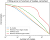 |
Fig. 4 Fitting error as a function of modes for different considered bases. |
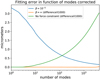 |
Fig. 5 Fitting error for classical KLs and force-optimised KLs. The green and orange curves show the fitting error difference with respect to the blue curve. |
6.2.2 Statistics on position and force
The safety checks on shell mirrors usually impose maximum values for actuator celerity, position amplitude, and force amplitude at any given time. Typical values for M4 are a few tens of microns for maximum positions stroke and a maximum force of about 1.5 N. A full analysis of the effect of these limits would require studying a full stroke budget and is reserved for a later work. In this section, we compute the RMS of positions and forces based on the hypothesis that phase screens following Van Karman statistics are projected on the KL modes. We analyse the effect of the algorithm choice on the distribution of the statistics. With this tool, we can compare bases. We qualify a basis as valid when both position and force RMS are taking reasonable values.
Figure 6 compares the RMS of positions for 4000 corrected modes and for the classical case (no force constraint = minimised position) and for two β settings for the force-optimised case. Six groups of actuators are visible as identified in Fig. 3, each with two zones: there is a rather flat part identical to all cases, which corresponds to the correction of the phase in the pupil. The shape of the curve corresponding to actuators outside the pupil differs and is influenced by the parameters of the algorithm.
Positions clearly tend to zero in the zone for the classical basis (no force constraint). For the force-optimised case without damping (β = ∞), the positions tend to have large and outstanding amplitudes outside the pupil. When we varied the damping parameter (β = 10−5 in Fig. 6), a compromise in positions was possible and we were able to limit the excursion of positions while having little influence on the force distribution, as shown in the next figure.
Figure 7 shows that the case without a force constraint (hence when positions are forced to be small) generates very strong forces on actuators outside the pupil. For the force-optimised cases, the forces are well contained and are weaker outside than inside the pupil. The green and orange curves are almost the same and demonstrate that it is interesting to apply the damping factor β to limit the position excursions while preserving optimum force distribution. These results give an idea of the trade-off that can be made for the optimal control in positions and forces of an adaptive shell mirror.
To illustrate the dependence of the force on spatial frequency, we show in Fig. 8 the maximum RMS of the force as a function of the number of corrected modes for the force-optimised KL basis with β = 10−5. This plot shows that up to about 700 modes, the forces are quite weak. In a regime up to 4200 modes, the dependence is almost linear with the number of modes. After 4200 corrected modes, the forces increase abruptly.
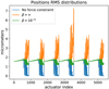 |
Fig. 6 Position distribution for force-optimised KLs with different β parameters. No force-constraint stands for original double -diagonalisation method with position minimisation. The assumption for the number of corrected modes is 4000. |
6.3 Minioning of outer shell actuators
The preceding section covered the nominal case in which all degrees of freedom (the 5352 actuators for M4) are directly controlled by the user. In most AO systems with an adaptive shell, the interface only permits accessing a limited number of degrees of freedom, for example 4866 inner actuators in the case of M4 (see Fig. 3). This excludes the three outer rings of actuators that are reserved for the internal M4 control. The positions of these actuators are determined as linear combinations of commands sent to the remaining (inner) actuators. This extrapolation policy is represented by a linear algorithm that is referred to as the minioning process. In the following, we outline the outer actuator minioning using zero-force policy. The recent report by Riccardi (2021) provides a more thorough account of different available options.
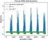 |
Fig. 7 Force distribution for force-optimised KLs with different β parameter and no force constraint. The assumption for the number of corrected modes is 4000. |
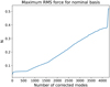 |
Fig. 8 Maximum force RMS as a function of the number of corrected modes for the force-optimised KL basis with β = 10−5. |
6.3.1 Zero-force policy on outer actuators
The zero-force policy on the outer M4 actuators consists of the following: the outer positions are adjusted such that the forces applied on them are rigorously zero while the inner actuators do not move. We compute the forces as
 (51)
(51)
where the forces and positions are explicitly decomposed into inner and outer actuators. The outer actuators are minioned by applying a zero-force to them, that is, f0 = 0. Solving for  , that is, the forces to apply to the inner actuators, we find
 (52)
(52)
and
 (53)
(53)
for outer actuator setpoints, ensuring that a zero-force policy is followed. From Eq. (53), we can write the minioning matrix M as
 (54)
(54)
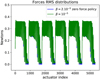 |
Fig. 9 Force distribution for force-optimised KLs with zero-force policy compared to the nominal case. The assumption for number of corrected modes is 4000. |
6.3.2 Modal basis computation with minioning
To account for the effect of the outer actuators on the OPD in the pupil, we define a modified influence matrix Hm[nact, ni], a reduced stiffness matrix Km [ni, ni], and a covariance matrix ![Mathematical equation: ${\bf{C}}_h^m\left[ {{n_i},{n_i}} \right]$](/articles/aa/full_html/2024/01/aa46902-23/aa46902-23-eq57.png) with the following definitions:
with the following definitions:
 (55)
(55)
In the case of the zero-force policy in Eq. (54), we can retrieve the result of Riccardi (2021) for the reduced stiffness matrix,
 (56)
(56)
The modal basis with minioning is obtained with the same calculations as in Sect. 4, but we replace H by Hm, K by Km, and Ch by  to obtain the full basis (Eq. (43)), which we call
 ![Mathematical equation: ${\bf{B}}_F^m\left[ {{n_i},{n_{{\rm{modes}}}}} \right]$](/articles/aa/full_html/2024/01/aa46902-23/aa46902-23-eq61.png) . It is expressed in the 4866 inner actuators and can be used for the control.
. It is expressed in the 4866 inner actuators and can be used for the control.
For the statistical analysis of the performance of the basis, we must express the basis on all actuators and execute the calculations of Sect. 5,
 (57)
(57)
We apply this zero-force policy and repeat the calculations of the basis and the statistical analysis. The damping parameter need to be slightly adjusted (β = 2 × 10⁻⁵) for the zero-force policy case. Figure 9 presents the force distribution with the zero-force policy basis compared to the nominal one. The force distributions are globally very similar, except when the forces are null by design. The difference is more visible for the positions, as shown in Fig. 10. The excursion of outer actuators for the zero-force policy is higher by about 15%, but still with values below the mean value over the pupil. This shows that in the case of the selection of 4866 actuators of M4, the zero-force policy does not lead to any significant deterioration of forces and positions statistics.
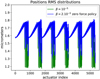 |
Fig. 10 Position distribution for force-optimised KLs with zero-force policy compared to the nominal case. The assumption for the number of corrected modes is 4000. |
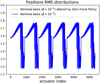 |
Fig. 11 Position distribution for a nominal basis alteration with zero-force policy compared to the nominal basis. The assumption for the number of corrected modes is 4000. There are 4866 inner actuators. |
6.3.3 Alternative: A posteriori modification of the nominal basis
Although the inner actuator setpoints are not affected by the zero-force policy, strictly speaking, the same is not true with the OPD induced by outer actuators. This justifies that in the general case, the method in Sect. 6.3.2 is used.
However, in the particular case of M4, the OPD induced by outer actuators is rather small. In this case, we can compute the nominal basis and alter it by applying the minioning, as in the following equation:
![Mathematical equation: ${\bf{B}}_F^{\,\bmod \,} = {\bf{M}} \cdot {{\bf{B}}_F}[i,:].$](/articles/aa/full_html/2024/01/aa46902-23/aa46902-23-eq63.png) (58)
(58)
Application of Eq. (58) mostly preserves the position and force statistics and only slightly affects the mode orthonormality (Co ≈ 0.01). This means that we can alternatively compute the KL basis (from Sect. 4 on 5352 actuators without enforcing any specific policy) without any minioning whatsoever and apply it to the basis a posteriori. The effect on positions and forces is shown in Figs. 11 and 12. We can verify that the forces indeed reach zero on the outer actuators. A slight increase of forces on inner actuators near the border is visible in detail. The positions are barely changed, which demonstrates that the nominal basis is very close to a zero-force policy.
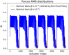 |
Fig. 12 Force distribution for a nominal basis alteration with zero-force policy compared to the nominal basis. The assumption for the number of corrected modes is 4000. There are 4866 inner actuators. |
7 Conclusion
This paper provides the mathematical foundations underpinning the generation of a set of bi-dimensional deformation modes suitable for the optimal control of force-constrained adaptive shell mirrors using the KL formalism. The latter was revisited using the double-diagonalisation method to compute the atmospheric turbulence (stochastic process) eigenfunctions expressed as a linear combination of the DM principal components (geometric force-dependent mechanical deformations). The use of force instead of actuator position control is the novelty we introduced. We developed the means for generating the bases orthogonal to specific modes (e.g. tip-tilt) and the subtleties of how to create them to minimise forces and avoid large positions.
The analysis conducted here confirmed that the new basis minimises force, as was expected by construction. Although the bi-dimensional modal deformations may be different from the classical calculation, the fitting error is by no means degraded (Fig. 5). We also showed how to balance force and mechanical excursion (i.e. position) by introducing regularisation. This acts as a damping parameter to maintain both force and position at reasonable values.
The formalism we used is suitable for vetting any control basis an instrument wishes to use in terms of correction efficiency, force, and mechanical excursion. This is an important contribution leading to the assessment of acceptable control bases when another than the one developed here is to be adopted.
Furthermore, our developments are capable of handling different force policies on actuators, as is commonly done with adaptive shell mirrors. This is so as long as they can be expressed as linear penalties in either position or force. We illustrated the application to a first-generation instrument on the ELT in the absence of any constraint policy or with a zero-force policy (Fig. 10). The assessment of the impact of different policies now under consideration for the ELT-M4 will be the subject of a forthcoming paper.
Acknowledgements
We warmly thank Cédric Taïssir Héritier for his help in the integration of the modal basis generation algorithms in the OOPAO code, available at https://github.com/cheritier/OOPAO.
Appendix A Covariance matrix Cp expressed in actuator position setpoint space
Eqs 21 and 23 show how the covariance matrix is used in the classical method. The method will be slightly different in the force-minimisation case, where Δ is non-invertible (when all actuators are selected).
The atmospheric statistics is taken into account by computing the covariance matrix of the projection h of the IFs on turbulent phase screens ϕ , like in Lai et al. (2000),
 (A.1)
(A.1)
The covariance matrix is
 (A.2)
(A.2)
where Cϕ[np, np] is the covariance matrix of the turbulent phase. For the classical method, the step from Ch to Cp, that is, from projection coefficients to DM position setpoints, was to our knowledge not explicitly described in Lai et al. (2000). Because any modes, and especially the KL modes, are ultimately expressed in Position setpoints, Cp is definitely the matrix to use in Eq. 23.
The expression of Cp is derived here. From Eq. 14 (with Γ = 0 when Δ is invertible), we have
 (A.3)
(A.3)
and using Eq. 21, we obtain
 (A.4)
(A.4)
Plugging Eq. A.2 into Eq. A.4 effectively means computing
 (A.5)
(A.5)
that is, the least-squares projection of the phase-covariance function in the space spanned by the DM IFs.
Using the Wiener-Khinchine theorem, we can compute the covariance function more efficiently in the Fourier space by noting
 (A.6)
(A.6)
where Wϕ is the 2D phase spatial power-spectral density indexed by κ = (κx, κy), and ͒ denotes Fourier-transformed variables. This property is reformulated in Appendix B as a set of computer-efficient matrix operations.
Appendix B Optimised algorithm for computing Ch for von Karman turbulence
In the expression of Ch, the covariance matrix Cϕ[np, np] appears. For an ELT with a typical IF resolution of 5cm, we have np ≈ 5 × 10⁵. This makes the matrix impractical to use. One solution of this problem was proposed in Lai et al. (2000), where each element of Ch was computed in a double integration in the direct space using the relation between covariance matrix and the structure function. We used a method in the Fourier space that was proposed by Gendron (1995). We present this method and show how it can be written in a matrix form that can be parallelised efficiently.
The Fourier transform (FT) of the covariance matrix of phase points is equal to the FT of the power spectrum of phase points (Wiener-Khintchine theorem),
 (B.1)
(B.1)
where κ is the 2D vector of spatial frequencies and its module κ = |κ|.
We define nf as the number of points in the Fourier domain. For a Nyquist sampling, we have nf = (2 × dim)2 at least, where dim is the linear dimension of the smallest array containing a pupil.
We define fmax = 0.5dim/diameter as the maximum spatial frequency that can be computed numerically. WvK(k) is a bi-dimensional function.
With the goal of expressing the math in matrix form, we define a vector Wi[nf] obtained from reshaping the matrix WvK(k) in a vector.
In the same way, we define ![Mathematical equation: ${\bf{\hat H}}\left[ {{n_f},{n_{act}}} \right]$](/articles/aa/full_html/2024/01/aa46902-23/aa46902-23-eq71.png) as the matrix form of the collection of vectors describing the Fourier transform of the IFs. We define also the matrix D[nf, nact] whose columns are the replication of nact times the vector W multiplied by some normalisation factor,
as the matrix form of the collection of vectors describing the Fourier transform of the IFs. We define also the matrix D[nf, nact] whose columns are the replication of nact times the vector W multiplied by some normalisation factor,
 (B.2)
(B.2)
After some developments using the Parseval theorem (see e.g. Ellerbroek (2002)), we can rewrite Eq. A.2 using the expressions in the Fourier domain (where ○ is the element-wise matrix multiplication, and MH is the hermitian transpose of a matrix),
 (B.3)
(B.3)
where (:) represents matrix derasterisation into a vector format. This matrix equation can easily be parallelised by block and by taking advantage of the fact that it is symmetric.
References
- Arsenault, R., Biasi, R., Gallieni, D., et al. 2006, SPIE Conf. Ser., 6272, 62720V [NASA ADS] [Google Scholar]
- Brusa, G., Riccardi, A., Wildi, F. P., et al. 2003, in Astronomical Adaptive Optics Systems and Applications, 5169 eds. R. K. Tyson, & M. Lloyd-Hart, International Society for Optics and Photonics (SPIE), 26 [Google Scholar]
- Close, L. M., Gasho, V., Kopon, D., et al. 2010, SPIE Conf. Ser., 7736, 773605 [NASA ADS] [Google Scholar]
- Conan, R., & Correia, C. 2014, SPIE Conf. Ser., 9148, 6 [Google Scholar]
- Conan, R., Borgnino, J., Ziad, A., & Martin, F. 2000, J. Opt. Soc. Am. A, 17, 1807 [NASA ADS] [CrossRef] [Google Scholar]
- Ellerbroek, B. L. 2002, J. Opt. Soc. Am. A, 19, 1803 [NASA ADS] [CrossRef] [Google Scholar]
- Ferreira, F., Gendron, E., Rousset, G., & Gratadour, D. 2018, A&A, 616, A102 [NASA ADS] [CrossRef] [EDP Sciences] [Google Scholar]
- Fontanella, L., & Ippoliti, L. 2012, in Handbook of Statistics, 30, Time Series Analysis: Methods and Applications, eds. T. Subba Rao, S. Subba Rao, & C. Rao (Elsevier), 497 [CrossRef] [Google Scholar]
- Gendron, E. 1995, PhD thesis, Paris [Google Scholar]
- Lai, O., Jr., P. J. S., & Gendron, E. 2000, in Adaptive Optical Systems Technology, 4007, ed. P. L. Wizinowich, International Society for Optics and Photonics (SPIE), 620 [Google Scholar]
- Riccardi, A. 2021, arXiv e-prints [arXiv:2101.04801] [Google Scholar]
- Riccardi, A., Xompero, M., Briguglio, R., et al. 2010, SPIE Conf. Ser., 7736, 77362C [Google Scholar]
- Salinari, P., Del Vecchio, C., & Biliotti, V. 1994, in European Southern Observatory Conference and Workshop Proceedings, 48, 247 [NASA ADS] [Google Scholar]
- Sasiela, R. J. 1994, Electromagnetic Wave Propagation in Turbulence (Springer Berlin, Heidelberg) [CrossRef] [Google Scholar]
- Upton, R., & Ellerbroek, B. 2004, Opt. Lett., 29, 2840 [NASA ADS] [CrossRef] [Google Scholar]
- Vernet, E., Cirasuolo, M., Cayrel, M., et al. 2019, The Messenger, 178, 3 [NASA ADS] [Google Scholar]
All Figures
|
Fig. 1 Face-on representation of the first 25 KL modes obtained from the eigenmodes of the piston-removed phase covariance matrix in Fig. 2. The first mode corresponds to a numerical leftover of the piston. |
| In the text | |
|
Fig. 2 Piston-removed zonal spatial covariance matrix using lexicographic indexing for a pupil shown in Fig. 1. The equation in the title corresponds to the development of 〈‖ϕ − ϕP‖2〉, where the piston mode is ϕP = P ⋅ P⊤ ⋅ ϕ. |
| In the text | |
|
Fig. 3 Top: ELT quaternary mirror (M4) geometry projected on the primary mirror (M1) coordinates and overlaid on the M1 pupil. Enlargement of one of the six independent sectors. Bottom: 5352 actuators column-wise indexed by lexicographical order. 1 indexes the blue dots (inner actuators), and 0 indexes the green dots (outer actuator). |
| In the text | |
|
Fig. 4 Fitting error as a function of modes for different considered bases. |
| In the text | |
|
Fig. 5 Fitting error for classical KLs and force-optimised KLs. The green and orange curves show the fitting error difference with respect to the blue curve. |
| In the text | |
|
Fig. 6 Position distribution for force-optimised KLs with different β parameters. No force-constraint stands for original double -diagonalisation method with position minimisation. The assumption for the number of corrected modes is 4000. |
| In the text | |
|
Fig. 7 Force distribution for force-optimised KLs with different β parameter and no force constraint. The assumption for the number of corrected modes is 4000. |
| In the text | |
|
Fig. 8 Maximum force RMS as a function of the number of corrected modes for the force-optimised KL basis with β = 10−5. |
| In the text | |
|
Fig. 9 Force distribution for force-optimised KLs with zero-force policy compared to the nominal case. The assumption for number of corrected modes is 4000. |
| In the text | |
|
Fig. 10 Position distribution for force-optimised KLs with zero-force policy compared to the nominal case. The assumption for the number of corrected modes is 4000. |
| In the text | |
|
Fig. 11 Position distribution for a nominal basis alteration with zero-force policy compared to the nominal basis. The assumption for the number of corrected modes is 4000. There are 4866 inner actuators. |
| In the text | |
|
Fig. 12 Force distribution for a nominal basis alteration with zero-force policy compared to the nominal basis. The assumption for the number of corrected modes is 4000. There are 4866 inner actuators. |
| In the text | |
Current usage metrics show cumulative count of Article Views (full-text article views including HTML views, PDF and ePub downloads, according to the available data) and Abstracts Views on Vision4Press platform.
Data correspond to usage on the plateform after 2015. The current usage metrics is available 48-96 hours after online publication and is updated daily on week days.
Initial download of the metrics may take a while.