| Issue |
A&A
Volume 681, January 2024
|
|
|---|---|---|
| Article Number | A123 | |
| Number of page(s) | 11 | |
| Section | Cosmology (including clusters of galaxies) | |
| DOI | https://doi.org/10.1051/0004-6361/202346734 | |
| Published online | 23 January 2024 | |
Fast emulation of cosmological density fields based on dimensionality reduction and supervised machine learning
1
Departamento de Física, Faculdade de Ciências, Universidade de Lisboa, Campo Grande, 1749-016 Lisboa, Portugal
e-mail: This email address is being protected from spambots. You need JavaScript enabled to view it.
2
Instituto de Astrofísica e Ciências do Espacço, Faculdade de Ciências, Universidade de Lisboa, Campo Grande, 1749-016 Lisboa, Portugal
3
Donald Bren School of Information and Computer Sciences, University of California, Irvine, CA 92697, USA
4
CENTRA, Faculdade de Ciências, Universidade de Lisboa, 1749-016 Lisboa, Portugal
5
Departamento de Física, ETSI Navales, Universidad Politécnica de Madrid, Avda. de la Memoria 4, 28040 Madrid, Spain
Received:
24
April
2023
Accepted:
21
August
2023
Abstract
N-body simulation is the most powerful method for studying the nonlinear evolution of large-scale structures. However, these simulations require a great deal of computational resources, making their direct adoption unfeasible in scenarios that require broad explorations of parameter spaces. In this work we show that it is possible to perform fast dark matter density field emulations with competitive accuracy using simple machine learning approaches. We built an emulator based on dimensionality reduction and machine learning regression combining simple principal component analysis and supervised learning methods. For the estimations with a single free parameter we trained on the dark matter density parameter, Ωm, while for emulations with two free parameters we trained on a range of Ωm and redshift. The method first adopts a projection of a grid of simulations on a given basis. Then, a machine learning regression is trained on this projected grid. Finally, new density cubes for different cosmological parameters can be estimated without relying directly on new N-body simulations by predicting and de-projecting the basis coefficients. We show that the proposed emulator can generate density cubes at nonlinear cosmological scales with density distributions within a few percent compared to the corresponding N-body simulations. The method enables gains of three orders of magnitude in CPU run times compared to performing a full N-body simulation while reproducing the power spectrum and bispectrum within ∼1% and ∼3%, respectively, for the single free parameter emulation and ∼5% and ∼15% for two free parameters. This can significantly accelerate the generation of density cubes for a wide variety of cosmological models, opening doors to previously unfeasible applications, for example parameter and model inferences at full survey scales, such as the ESA/NASA Euclid mission.
Key words: large-scale structure of Universe / cosmology: miscellaneous / methods: statistical / methods: numerical
© The Authors 2024
 Open Access article, published by EDP Sciences, under the terms of the Creative Commons Attribution License (https://creativecommons.org/licenses/by/4.0), which permits unrestricted use, distribution, and reproduction in any medium, provided the original work is properly cited.
This article is published in open access under the Subscribe to Open model. This email address is being protected from spambots. You need JavaScript enabled to view it. to support open access publication.
1. Introduction
Numerical N-body simulation is arguably the most powerful method to describe the formation and evolution of cosmological structure, especially at late times when the growth of perturbations, driven by gravitational collapse, becomes highly nonlinear. These simulations provide high-accuracy predictions on how the dark matter (DM) density and velocity fields evolve, allowing the identification of model signatures and observables that can be compared against observations. This process often requires the generation of a very large number of computationally intensive simulation runs, posing a prohibitive bottleneck on the number of simulated models that can be explored in the preparation and scientific exploitation of modern cosmological surveys. This penalizes model inference studies, specially using Bayesian methods considering the shear data volume of modern sky surveys such as ESA/Gaia (Gaia Collaboration 2016, 2023) and ESA/Euclid (Laureijs et al. 2011; Euclid Collaboration 2022), and time-resolved surveys such as the Zwicky Transient Facility (Bellm & Kulkarni 2017) and LSST/Rubinkllk (Ivezić et al. 2019).
One typical way to address these types of challenges is through the adoption of simulation emulators. These emulators try to reproduce the output of a simulator by the adoption of multiple regression methodologies (e.g., O’Hagan & Kingman 1978). Gaussian processes, for instance, have been used in such scenarios (e.g., Currin et al. 1988, 1991). More recently, attention has been shifted to the machine learning (ML) approach, where deep models populate most of the density field emulation landscape.
Emulation of dark matter density fields with deep learning techniques such as the Generative Adversarial Networks (GANs) or Variational Auto-Encoders (VAEs) methods have been proposed, in 2D (e.g., Rodríguez et al. 2018; Ullmo et al. 2021) and 3D (e.g., Perraudin et al. 2019). These methods show that it is possible to use deep learning to emulate DM density fields using the Lagrangian approach (e.g., He et al. 2019; Giusarma et al. 2023; Alves de Oliveira et al. 2020; Kodi Ramanah et al. 2020; Jamieson et al. 2023), instead of the less general Eulerian approach. The emerging picture is that deep learning models tend to efficiently emulate DM fields, but generally require large training sets. Their accuracy starts to degrade below scales k ≃ 1 h Mpc−1, that is, slightly inside the strong nonlinear regime of structure formation. Other works (e.g., Conceição et al. 2021, 2022) focused on the emulation and resolution enhancement of N-body simulations using these methods with minimal computational resources.
Although the deep learning approach enables the decrease in time and computational resources needed to obtain an output similar to that of an N-body simulation, it still remains a reasonably complex approach that is often difficult to interpret. Since the N-body density fields usually consist of extremely large arrays that contain millions of matter density values with a fair degree of nonlinear behavior, it is compelling to think that only deep models should be able to handle such data. However, considering that we are dealing with nonrandom data with a high degree of symmetry brought by the cosmological principle, it should be possible to take advantage of the redundancy in this data, compressing it in a more compact basis. Using this reduced data representation, it becomes more feasible to apply simpler machine learning models, decreasing further the amount of computational resources and time needed to obtain the outputs, and hopefully increasing the interpretability of the models.
In this work we propose a methodology that aims to achieve these goals. Our methodology first adopts a simple data projection method, principal component analysis (PCA; Pearson 1901; Hotelling 1933; Jollife 2002), to project the N-body training data into a smaller basis of coefficients called Principal Components (PCs), and then uses the transformed representation as an input to a set of simple and interpretable supervised learning methods: random forests (RF; Breiman 2001), extremely randomized trees (ERTs; Geurts et al. 2006), shallow neural networks (NNs; McCulloch & Pitts 1943) and support vector machines (SVMs; Cortes & Vapnik 1995).
We tested our methodology in two different scenarios. In the first we performed the emulations using the dark matter density (Ωm) as a single free parameter. In the second scenario we slightly increased our dataset and included the redshift z as an additional free parameter, enabling us to test the generalization capacity of our models under higher-dimensional contexts. To gauge the performance of the trained models and of our proposed methodology in general, we compare the power spectrum and bispectrum of our emulations with that of an N-body simulation generated for the same cosmology and initial conditions. In this way, we ensure that our emulated density fields have statistical properties as close to those of the true simulation as possible, on large and small scales.
In this paper we present our proposed methodology and the adopted comparison metrics in Sect. 2. We show the results of its application to emulate N-body simulation density fields in Sect. 3. Then, we present a brief discussion of the computational efficiency of our method in Sect. 4. Finally, we present our conclusions in Sect. 5.
2. Methodology
A consequence of the highly redundant amount of information present within the large-scale structure of the Universe is that this information can be highly compressible. Accordingly, the density field emulator design described in this section is based first on the application of a dimensionality reduction method and then on a supervised machine learning method. These methods require the construction of a training (and test) set of N-body simulations and evaluation metrics that we also describe in this section.
2.1. The density field emulator
2.1.1. PCA projection
We started from a library of k density fields, each created from an independent N-body simulation with parameters Dk. Each cube of size n3 of this library is rearranged into a row of a matrix Mk × n3, with k rows and n3 columns. The first step in our methodology was to solve a data compression problem: how to find a sparser representation Sk × l of the matrix M, with l ⋘ n and l ≤ k. We applied PCA, which is a very simple and well-established methodology adopted in multiple contexts in astronomy (e.g., Steiner et al. 2009; Ishida & de Souza 2011; Krone-Martins & Moitinho 2014; Euclid Collaboration 2021; Conceição et al. 2021, 2022) to perform this compression. We note, though, that although we adopted PCA here for simplicity, any other invertible dimensionality reduction or compression method could be used. To perform the PCA, we adopted a singular value decomposition. It decomposes the M matrix in three matrices M = UZVT, where U is an unitary k × k matrix, Z is a diagonal matrix with the singular values, and V is a n3 × k matrix containing the eigenvectors of the covariance matrix in each column, which are the principal directions. The principal components (e.g., MV or equivalently UZ) are obtained by projecting the data in the principal directions. The crucial step when performing the dimensionality reduction is to select the first l columns of U and the left-right l × l block of Z. Their product gives us our Sk × l matrix with the first l principal components, capturing most of the data variance. The reconstruction or decompression can be performed with the first l PCs by multiplying S by the transpose of the matrix V, VT.
2.1.2. Supervised learning regression
The second step of our methodology is to solve a regression problem, that is, to find a map f := D → S. Thus, given any set i of cosmological parameters Di, it is possible to estimate the compressed field Si, which after decompression generates an estimation of the density field Mi as if we had executed a full N-body simulation with the parameters Di. To construct this map, we studied four supervised machine learning algorithms in this work: ERT, RF, NN and SVM. Our motivation to use multiple methods is to compare the emulation yields obtained with them in this first exploratory study, since they could, in principle, present better results in different subdomains of the parameter space and in different scales of the density field. That could justify, in a future study, the construction of more precise ensembles (e.g., Mendes-Moreira et al. 2012).
The adoption of supervised learning methods in astronomy has a long history (e.g., Djorgovski et al. 2022). Neural networks (McCulloch & Pitts 1943) and support vector machines (Cortes & Vapnik 1995) are classical methods that have been successfully used in multiple contexts. For instance, before the recent boom in citations to computer science works in astronomical papers (Veneri et al. 2022), mostly due to the spread of deep learning approaches, NNs had already been used for almost four decades in astronomy, in optimization (Jeffrey & Rosner 1986), in heliophysics (Koons & Gorney 1990), adaptive optics (Angel et al. 1990; Sandler et al. 1991), star–galaxy separation (Odewahn et al. 1992), and galaxy classification (Storrie-Lombardi et al. 1992). Support vector machines, on the other hand, started to be used almost exclusively in extragalactic contexts in the 2000s (e.g., Zhang et al. 2002; Wadadekar 2005; Tsalmantza et al. 2007; Huertas-Company et al. 2008; Krone-Martins et al. 2008; Bailer-Jones et al. 2008), but they were also adopted in the classification of transients (Mahabal et al. 2008), stellar classification (e.g., Smith et al. 2010), interstellar medium structure (Beaumont et al. 2011), and heliophysics (e.g., Alipour et al. 2012), among others.
Random Forests (Ho 1995; Breiman 2001) started to be used in astronomy in the early 2000s. Like SVMs, they were first used in an extragalactic context to search for quasars (Breiman et al. 2003) and supernovae (Bailey et al. 2007), to identify high-energy sources (Scaringi et al. 2008), and to perform photometric redshift estimation (Carliles et al. 2010), but they later found other applications such as variable star classification (Richards et al. 2011; Dubath et al. 2011), feature selection for stellar membership analysis (Sarro et al. 2014), anomaly detection (Nun et al. 2014), and young stellar object classification including missing data (Ducourant et al. 2017). Finally, the last method adopted here, extremely randomized trees (Geurts et al. 2006), is a supervised learning method that is a variant of the more commonly used RF. Although not as widely adopted in astronomy as the other methods, in the past decade ERTs have been successfully used in the context of stellar astrophysical parameter determination (Bailer-Jones et al. 2013; Delchambre 2018), quasar selection (Graham et al. 2014), prediction of galaxy properties from dark matter halo simulations (Kamdar et al. 2016), and the discovery of new gravitationally lensed quasars (Krone-Martins et al. 2018; Delchambre et al. 2019). Like RFs, ERTs are based on ensembles of decision trees, but they split the trees differently: RFs split trees deterministically, while the ERT splits are chosen entirely at random (Geurts et al. 2006).
2.1.3. Algorithm optimization
As with most machine learning methods, supervised learning algorithms depend on hyper-parameters that can be optimized. For each method, balancing hyper-parameters can be important to improve the speed and performance of the method. To optimize them, we explored each method’s hyper-parameter space with different optimization schemes. We chose to experiment with the standard grid-search approach (e.g., Lecun et al. 1998; Bergstra & Bengio 2012), bootstrap aggregating (e.g., Breiman 1996), and k-fold cross-validation (K-CV; e.g., Hastie et al. 2009) optimization methods. Each optimization method provides a different optimal model. To discriminate between them, we compared the best emulation from each method with the corresponding ground truth test simulation using the cosmological power spectrum (see Sect. 2.4). For this, we define the power spectrum distance ratio metric as
 (1)
(1)
where n is the power spectrum vector size,  and
and  are respectively the estimated and simulated power spectrum of the ith wave mode, ki. Consequently, we take as the best performing optimization method the one providing the smallest D.
The application of these methods to the different supervised learning variants of our emulator involves optimizations over different sets of hyper-parameters. Our choice of hyper-parameters and methodology, in each case, was as follows.
For the RF method, the hyper-parameter optimization was on the number of trees in the ensemble (ntree), the minimum number of observations allowed in the terminal leaves of the trees (nodesize), and the number of independent variables randomly sampled as candidates for each split (mtry). Therefore, the optimization of the last parameter is only possible for regression problems with more than one independent variable (i.e., in the case of emulations in Ωm and z). To perform the search over this hyper-parameter space, we first performed a simple grid-search over the number of trees for the values ntree = (500, 1000, 2000), fixed the best performing value, and proceeded to optimize the remaining hyper-parameters, experimenting with both bootstrap and k-fold cross-validation. This procedure was implemented using the e1071 package (Meyer et al. 2021).
For the ERTs, our optimization approach is similar to the RF case, except that instead of optimizing nodesize, we optimized the number of random splits considered at each partitioning node of the tree (numRandomCuts). Then the optimization proceeded in similar way to that of RF. First, by fixing ntree with a grid-search over the same possibilities, followed by a search over mtry and numRandomCuts and experimenting with the same optimization schemes. This procedure was implemented using the caret package (Kuhn 2008).
For the NNs we decided to use a single-layer network as our aim is to study the simplest possible architectures. We optimized the parameter size, corresponding to the number of nodes in the single hidden layer, and the parameter decay, corresponding to a regularization constant in the weight decay formula, which constrains the number of free parameters (weights) in the NN model.
Finally, for the SVMs we first performed a grid-search over the different kernel possibilities, with the remaining hyper-parameters set to their default values. After finding the optimal kernel, we optimized the standard SVM hyper-parameters cost and gamma.
2.2. Training and test datasets
One advantage of our emulation method is that it is a simple and generalizable approach to the emulation of N-body density fields. To demonstrate the flexibility of the method, we decided to make all computations on a simple computer system (a quad-core Intel core i5 with 16Gb of RAM and no discrete GPUs) running Linux. We therefore planned our set of N-body simulation runs to use for the training of our emulator, with size and resolution specifications capable of resolving a range of nonlinear evolving cosmological scales in the chosen platform.
Our simulations were generated for a family of cosmological models based on the flat cold dark matter (CDM), Λ-CDM cosmology with Hubble parameter h = 0.7 and dark matter density parameter Ωdm = Ωm = 1 − ΩΛ, where Ωm is the total matter parameter and ΩΛ is the energy density parameter associated with the cosmological constant. In this way the energy density of radiation is neglected and baryons are treated in the simulations as collisionless dark matter. The initial conditions matter power spectrum was modeled with the CDM BBKS transfer function with a shape parameter given by Γ = Ωm h (Bardeen et al. 1986; Sugiyama 1995) and a normalization controlled by the σ8 parameter, which is the square root of the variance of the smoothed overdensity field on scales of 8 h−1 Mpc at present. The primordial power spectrum index of scalar perturbations was set to ns = 1. The simulation runs were generated with the Hydra public code (Couchman et al. 1995) that implements an adaptive mesh refinement AP3M method to compute gravitational forces and evolves a set of CDM mass particles in serial mode. We used the cosmic initial conditions generator provided in the Hydra code package to generate fields for 1603 particles of dark matter in a cubic volume with comoving length L = 100 h−1 Mpc on the side. In physical coordinates the simulation’s gravitational softening was held fixed to 25 h−1 kpc up to z = 1, and scaled as 50(1 + z)−1 h−1 kpc above this redshift. With this choice of parameters and force resolution, our simulations could in principle resolve scales, in high-density regions, within a minimum and maximum wave mode of about kmin ≃ 0.06 h Mpc−1 and kmax ≃ 30 h Mpc−1, respectively. All our simulation runs share the same initial conditions seed and start from an initial snapshot realization at z = 49 that is evolved until z = 0.
Our training dataset consists of 23 simulations with Ωm taking values in the interval Ωm ∈ [0.05, 0.6] with a regular separation equal to ΔΩm = 0.025. All other parameters were held fixed, with the exception of the primordial shape parameter that varied according to Γ = Ωm h. For each of these runs we store ten snapshots (cubic volumes) containing particle positions and velocities at each redshift. Our test dataset consists of a single simulation with Ωm = 0.31 and the same parameter setup, to be used as the ground truth. Before using all these runs with our emulation pipeline we first needed to sample the dark matter densities on a regular cubic grid for all snapshots. Hydra is a particle-based code that follows volume elements (the particles) using a Lagrangean description, so it does not provide densities directly. To convert these into a Eulerian grid of densities, we adopted a mass-assignment scheme that treats dark matter as smoothed particle hydrodynamics (SPH; Lucy 1977; Monaghan 1992) particles. For this, we used the darkdens code in Hydra to compute smoothing lengths, and a fast SPH grid method based on the mapping algorithm in da Silva et al. (2001) and Ramos et al. (2012). For the purpose of this work, we adopted a regular grid with 1283 voxels inside the simulation volume, which is grid choice that limits the resolution in our emulations to a maximum wave mode of about kmax ≃ 3 h Mpc−1. Finally, our simulation training set is therefore a template of simulations cubes, all with 1283 voxels, spanning a range of 23 values of Ωm and 10 values of z (which amounts to a total of 230 simulation cubes). In practice, we work with different subsets of these data for the cases of emulations with one or two free parameters, as described below.
2.3. Emulation pipeline
The first step in our emulation pipeline is to project our training dataset with PCA. We concatenate simulation arrays as vectors containing the base-10 logarithm of the density cubes. The vectors are then put in a matrix form before applying the PCA method with the data re-scaled and centered.
For emulations with a single free parameter at a fixed redshift (i.e., with Ωm), this procedure leads to 23 PCs for each simulation. We chose to preserve the total number of PCs in order to maintain the total amount of information of each simulation. After the PCA was implemented we obtained a new training dataset, with 23 PCs for each of the 23 simulations, represented in a 23 × 23 matrix. Once the training data was projected in its principle component representation we used the PCs to build and optimize the supervised learning algorithms. Since the density fields are represented by PCs, and our aim was to estimate the field itself, the training was performed using the PCs as dependent variables and Ωm as independent variables. To achieve this, we created a 23 iteration loop where in each iteration our algorithms build a regression model accounting for that specific PC and the same constant set of Ωm values. For the case of the NNs, the data was re-scaled to the Alipour et al. (2012) range to reduce the chances of getting stuck in local minima. After obtaining the new PCs, the final estimated cube was obtained by de-projecting them onto the original representation using the inverse de-projection operations:
 (2)
(2)
where S, L, s, and c, are the scores, loadings, scaling, and centering matrices and vectors, respectively.
For emulations with two parameters, the main difference with the one free parameter case is the size of the training dataset. To incorporate the training in redshift for the chosen computer platform, we decided to use only four redshifts, z = [0, 0.25, 0.75, 1] from our initial dataset. This translated into including four of the ten generated N-body snapshots in the training dataset, for each of the 23 simulations. For each of these redshifts we kept the same 23 Ωm density cubes we had in the case of regressions with a single parameter, Ωm. Our training dataset therefore had 23 × 4 = 92 simulation cubes, and we kept the cube with Ωm = 0.31 and z = 0.5 to compare emulation results against the corresponding simulation ground truth. The whole pipeline took a significantly longer time to run in this case: our dataset was significantly larger as it involved working on the basis of 92 PCs, instead of only 23 for the single free parameter emulation. Once again we chose to maintain all of the 92 PCs to perform the ML regressions, so in this case our training dataset was contained in a 23 × 92 matrix. We note that in this case we were making predictions using z and Ωm, while in the case of the Ωm single free parameter emulations we only used 23 simulations for training at each redshift.
Our emulation pipeline was fully written in the R programming language (R Core Team 2021). This includes the module of PCA decomposition, implementation of the different supervised regression algorithms, optimization with the grid-search, bootstrap, aggregating, and k-fold cross-validation methods, and finally density cube emulations using up to two free parameters.
2.4. Evaluation statistics
To assess the performance of our emulation method, we compare in Sect. 3 the power spectrum and bispectrum of our emulated volumes with those of the ground truth simulations. The power spectrum statistic is also used as part of our optimization of the method, as described in Sect. 2.1.3.
The power spectrum is the Fourier transform of the two-point correlation function
 (3)
(3)
where V is the box volume and
 (4)
(4)
is the power spectrum. For a Gaussian distribution of densities, P(k, z) provides a complete statistical description of the density field. However, the density field in N-body simulations in not Gaussian due to the nonlinear growth of cosmic structure. We compute the nonlinear power spectrum of the emulations and ground truth simulations with the public version of the powmes code (Colombi et al. 2009).
To measure departures from non-Gaussianity, we also computed the bispectrum of the density cubes. The bispectrum is associated with the Fourier transform of the three-point correlation function and, as a higher-order correlation function, it is sensitive to the nonlinear growth of cosmic structure. It is usually defined as B (see, e.g., Sefusatti et al. 2006)
 (5)
(5)
where δD, the Kronecker delta function, imposes a triangular relation between wave-mode vectors, k1 + k2 = −k3. Here we adopt a configuration of wave modes where k1 and k2 have fixed magnitudes, k1 = |k1| = 0.5 h Mpc−1 and k2 = |k2| = 0.6 h Mpc−1, and k3 = |k3| varies with the angle θ between k1 and k2. Our choice of wave-mode amplitudes differs from that in Kodi Ramanah et al. (2020) and Giusarma et al. (2023) because our simulation’s boxsize is smaller. This improves the statistics of our bispectrum determinations on the scales being probed by galaxy clustering surveys. Nevertheless, we checked that our bispectrum results agree with those in Kodi Ramanah et al. (2020) and Giusarma et al. (2023) for their choice of wave modes k1 = |k1| = 0.15 h Mpc−1 and k2 = |k2| = 0.25 h Mpc−1. In this work we use the Pylians3 public software1 to compute the bispectra presented in Sect. 3.
3. Results
In this section we present our main results. We show how each of our estimated density fields compares against the simulated density field using their power spectra and bispectra as comparison metrics. For the single free parameter case, we present the results concerning the implementation of our pipeline at four different redshifts.
3.1. The single free parameter case
For emulations with a single free parameter, we first show a visual comparison of one of our emulations (the best performing one) with the actual ground truth simulation in Fig. 1, where it is possible to see a remarkable similarity between the two representations. This figure shows the base-10 logarithm of the overdensity fields for the ground truth simulation (top left) and the NN emulation with one free parameter (top right). The overdensities are in units of the mean background density ⟨ρ⟩, that is, they are voxel overdensities Δ = ρ/⟨ρ⟩. The bottom panel shows the relative difference between the density of these cubes, (ρGT − ρNN)/ρGT.
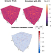 |
Fig. 1. Visual representation of the ground truth simulation (top left) against our NN emulation (top right), and the difference between them (bottom) at redshift z = 0. The mapped quantities are (top) the base-10 logarithm of the overdensity field Δ = ρ/⟨ρ⟩, where ⟨ρ⟩ is the mean background density, and (bottom) the fractional difference between the densities in sense ground truth density field ρGT minus the NN emulation ρNN. |
Moving now toward a more quantitative description, we show in Fig. 2 the distribution of the base-10 logarithm of the voxel overdensities Δ in the emulated and ground truth volumes represented in Fig. 1. The distributions (in the top panel) are clearly non-Gaussian and their ratios (in the bottom panel) indicate that the emulator performs best in the range of densities that are more frequent in the simulated volume. This result confirms expectations because the tails of the distributions are rare over- and underdensities (in high-density structures or deep voids) that are also underrepresented in the training dataset. Nevertheless, the agreement between the distributions is remarkable, especially if we take into account that this emulation was done with a training dataset with only 23 density cubes and a NN geometry with a single hidden layer. The differences are typically below 2.5% in the range 0.01⟨Δ⟩100. Outside this range, where densities correspond to voxels inside collapsed halos and deep voids, the agreement between distributions is still better than 5%.
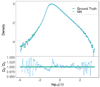 |
Fig. 2. Comparison of the NN emulation against the ground truth simulation using the logarithmic overdensity distribution. Top panel: distribution of the base-10 logarithm of voxel overdensities in the ground truth simulation and emulation volume represented in Fig. 1. Bottom panel: ratio of the distribution functions displayed in the top panel. The ratio Δ = ρ/⟨ρ⟩ is the overdensity contrast. |
Figure 3 shows the power spectrum from emulations with one free parameter, Ωm = 0.31, at fixed redshifts, z = 0 (top left), z = 0.5 (top right), z = 1 (bottom left), and z = 10 (bottom right). In each plot the top panel shows the power spectra of the ground truth simulation and our emulator implementations, featuring ERTs, NNs, RF, and SVMs as supervised learning algorithms. The bottom panel in each plot shows the ratio of the power spectrum of different emulator methods to the ground truth power spectrum.
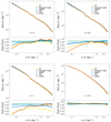 |
Fig. 3. Power spectrum emulations at redshifts z = 0 (top left), z = 0.5 (top right), z = 1 (bottom left), and z = 10 (bottom right) for model regressions with a single parameter, Ωm = 0.31. The top panel of each plot shows the power spectra obtained with our different emulation variants, extremely randomized trees (ET), neural networks (NN), Random Forests (RF), and support vector machines (SVM). The bottom panel in each plot shows the ratio of the power in each emulation to the power in the ground truth N-body simulation (PE(k) = Estimated; PS(k) = Simulated). |
Overall, the NN is our best performing algorithm; it achieves an accuracy above 99% at all redshifts and for most of the k domain. Random Forests manages to show similar accuracy at all redshifts except at z = 1 where performance decreases slightly, but still achieves ratios above the 96% level at all k. The other algorithms have somewhat worse performance, particularly at z = 0.5 and z = 1. At z = 10 all algorithms show a strong agreement with the power spectrum of the ground truth simulation. This agrees with expectations because most of the resolved scales in our simulations are still evolving linearly at that epoch, and therefore strong underrepresented over- and underdensities do not have enough time to form by that redshift. In light of this argument one could expect larger power spectrum deviations as redshift decreases because progressively larger nonlinearities develop at low z. Our results seem to contradict this trend at redshift z = 0.5 and below, because the different power spectrum ratios in Fig. 3, generally, tend to approach 1 as redshift decreases. This apparent contradiction can still be understood as a consequence of the level of representation (amount) of nonlinearities in the training set if we take into consideration the dynamics of the ΛCDM model at z < 1. Below this redshift, the cosmological constant reverts the Hubble expansion rate from a decelerated phase, due to matter domination, into an accelerated expansion. As larger over- and underdensities develop inside our probed volume, their number is better represented in the training set below this redshift than at higher-z (where structure grows in a decelerating matter-dominated universe).
Another interesting feature of our results is the decrease in power spectrum ratios at small k, that is, at large scales. This trend is common to all algorithms, and again can be interpreted as a lack of independent modes in the training dataset.
Figure 4 presents the results from our bispectrum analysis. As before, the figure shows bispectra and bispetra ratios at redshifts z = 0 (top left), z = 0.5 (top right), z = 1 (bottom left), and z = 10 (bottom right), for the Ωm = 0.31 cosmology. On the x-axis, θ is the angle between the wave modes k1 and k2 of our bispectra configuration (see Sect. 2.4). The relative performance of the algorithms is similar to the power spectrum results. The NN tends to be the best performing algorithm, followed closely by the RF implementation, whereas the other algorithms show lower performance. Our results also show that at the extremes of the θ domain the different algorithms also tend to underperform, especially at large θ. The level of disagreement between emulated and ground truth bispectra is also greater than in the case of the power spectrum. The larger deviations from the ground truth are a consequence of the larger uncertainties, generally, associated with the measurement of tree-point, and other higher-order, correlation functions from a finite volume. On the other hand, the larger deviations at large θ are linked to the choice of our bispectrum configuration, where k1 = 0.5 h Mpc−1 and k2 = 0.6 h Mpc−1 were set to scales that are closer to the lower end of the k domain in our simulations, and therefore correspond to larger scales that are less represented in our training set.
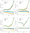 |
Fig. 4. Bipectrum emulations at redshifts z = 0 (top left), z = 0.5 (top right), z = 1 (bottom left), and z = 10 (bottom right) for model regressions with a single parameter, Ωm = 0.31. The top panel of each plot shows bispectra for our different emulation variants, extremely randomized trees (ET), neural networks (NN), Random Forests (RF), and support vector machines (SVM). The bottom panel in each plot shows the bispectra ratios from emulations, BE(θ), and the BS(θ) the ground truth simulation. |
3.2. The two free parameters case
In an attempt to expand the cosmological parameter space of our emulation method and test it under higher-dimensional settings, we included the redshift as an additional free parameter in our emulation pipeline. Here we present results for emulations at Ωm = 0.31 and z = 0.5.
Figure 5 shows the power spectrum (top panel) and power spectrum ratios (bottom panel) of our emulator variants (ET, NN, RF, SVM) versus the ground truth simulations. As expected, there is a general decrease in performance of the algorithms due to the increased dimensionality of the problem. NN is no longer the best performing algorithm, with errors reaching 25% at around k = 0.6 h Mpc−1. The RF and NN algorithms both overestimate the power spectrum in the range around 0.1 h Mpc−1 ≤ k ≤ 2 h Mpc−1, while SVM and ET consistently underestimate it.
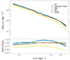 |
Fig. 5. Power spectra of the estimated density field using the four algorithms (ET, NN, RF, SVM) on the two free parameters dataset (Ωm,z) at Ωm = 0.31 and z = 0.5. Top panel: power spectra curves. Bottom panel: power spectra ratio (PE(k) = Estimated; PS(k) = Simulated). |
For our emulation setup with two free parameters, the SVM is by far the best performing algorithm. It achieves an accuracy of more than 95% for 0.3 h Mpc−1 ≤ k ≤ 2 h Mpc−1, decreasing to about 90% at the high-k (small-scale) extreme and ∼85% at the low-k (large-scale) extreme. This suggests an advantage of this algorithm for applications in multi-dimensional datasets, in particular, due to its adoption of nonlinear kernels before the hyper-plane segregation.
The degradation of results with the increase in dimension of the emulation problem is a consequence of the curse of dimensionality (Bellman et al. 1957) that affects most optimization methods, and thus also supervised learning methods. This problem translates the need of increasing the size of the training set exponentially when adding dimensions in the feature space so that a similar performance to the lower-dimensional can be maintained. In this work our choice of computer platform limits the augmentation of the training set for emulations with two parameters to a factor of only four times the size of the training set of our one free parameter case. To maintain the high degree of accuracy of the single parameter case, we should further increase the size of the training dataset.
Our bispectrum results for emulations with two free parameters are shown in Fig. 6. As before, the top panels show bispectra curves, whereas the bottom panel shows bispectra ratios (BE(k) = Estimated, BS(k) = Simulated bispectra). A striking feature is that all algorithms except ET overestimate the bispectrum, something that does not happen in the one parameter emulation scenario. Since ET is the only algorithm that considers only one of the independent variables, redshift or Ωm, the other algorithms may be overestimating the bispectrum due to a degeneracy between the two parameters. The self-similarity of cosmological structure induced by gravity-only simulations leads to some degree of degeneracy between the redshift epoch and Ωm for a given scale of observation. A snapshot at high redshift with a given Ωm displays a distribution of densities similar to a lower-redshift snapshot with a lower Ωm. This is an approximate argument that does not take into consideration the impact of Ωm on the epoch of transition from matter to cosmological constant domination (which happens at different z for different Ωm), but generally applies to simulation snapshots away from these transition redshifts.
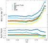 |
Fig. 6. Bispectra of the estimated density field using the four algorithms(ET, NN, RF, SVM) on the two free parameters (Ωm, z) at Ωm = 0.31 and z = 0.5. Top panel: bispectra curves. Bottom panel: bispectra ratio (BE(θ) = Estimated; BS(θ) = Simulated). |
These results further indicate that SVMs are the best method among those studied in this work since, as we can see, even when considering higher-order correlations it still out-performs the other algorithms. It is the only algorithm able to maintain an accuracy above 85% for the entire θ domain.
4. Discussion
In this section we discuss some of our key findings. We first discuss the computational efficiency of our methods, as measured by CPU run times. Subsequently, we analyze the algorithms employed in our investigation, providing a detailed assessment of their performance and potential for application in related research. Finally, we conclude by outlining possible avenues for improvements in our approach.
4.1. Efficiency
In Table 1 we present the CPU run times for the best performing algorithms in both emulation cases considered in this work. These cases correspond first to considering Ωm as a single free parameter (first row of the table) and then to using both Ωm and z as free parameters (second row). For the single free parameter case, we present the results trained with the dataset of 23 simulation snapshots at z = 0. The run times shown in the table correspond to both the PC estimation and to the de-projection into the final emulated density field, and we also present the sum of the two as the “Total emulation time” column.
CPU run times for the emulation step our proposed N-body density field emulation pipeline.
In terms of pure computational efficiency, the outcomes of our emulation pipeline seem highly satisfactory, particularly when considering that an N-body simulation of a similar scale requires 84 min to complete using the same system used for our emulation experiments. As exemplified in Table 1, the total emulation times for the single parameter scenario and two free parameters scenario were on the order of 0.8 and 4.5 s, respectively. This represents a substantial improvement in efficiency as our proposed approach is three orders of magnitude faster than the corresponding N-body simulation run time.
4.2. Algorithms
The supervised learning algorithms used in this study warrant some discussion, as some noteworthy observations can be made.
First, our results indicate that the RF algorithm was successful at reproducing the statistical properties of the density fields, particularly the non-Gaussian features, as evidenced by the bispectrum results in Fig. 4 for the single free parameter case. However, the opposite behavior is observed in the two free parameters scenario, where RF significantly underperforms in comparison to the other methods. In contrast, the ERT algorithm yields consistently disappointing results across both parametric contexts, emerging as one of the poorest performers, which we find surprising given its conceptual similarity to RF.
Second, the NN and SVM algorithms stand out as both demonstrate superior performance in their respective contexts. NN yields the best results for the one-dimensional N-body regression case, as depicted in Figs. 3 and 4. Meanwhile, SVM outperforms all the other methods in the multi-dimensional regression context. Considering that our current cosmological models incorporate multiple parameters beyond those examined in this first study (e.g., Hubble constant, baryonic matter density, power spectrum normalization, spectral index), SVM seems to be a promising method in the more realistic high-dimensional context.
However, these results do not yet allow for definitive conclusions regarding the potential of these supervised algorithms. It is important to keep in mind that our hyper-parameter optimization process may not have achieved a global minimum in the regression error metrics and the algorithm cost functions. As our simple search was restricted to a constrained and finite range of hyper-parameter values, there is a possibility that the algorithms were confined to a local minimum, with further potential for improvement through a better and larger exploration of the hyper-parameter space. Nonetheless, our findings offer some indications of the potential of the analyzed algorithms.
4.3. Future prospects
There are several potential avenues to improve or extend the methods used in this study. Some of these improvements could be implemented without significant modifications to the existing pipeline. For example, one option would be to expand the parameter space to include additional cosmological parameters such as the Hubble constant or spectral index. Naturally, this would also require an increase in the training set to sample the parameter space. Alternatively, the dark matter density fields could be emulated with the inclusion of hydrodynamics, which would similarly require a substantial increase in training data. While hydrodynamics are known to introduce highly nonlinear effects that may be difficult to reproduce, the overall structure of the pipeline should remain very similar, perhaps only requiring the adoption of more advanced dimensionality reduction methods.
On the other hand, methods similar to those proposed here could also be coupled directly within N-body codes, perhaps to accelerate certain aspects of the simulation, such as certain scales of the simulation. This would naturally require more extensive modification to the pipeline and of the N-body codes.
Finally, an interesting application of our proposed methods that we are currently investigating involves attempting to emulate the hydrodynamics directly from dark matter-only simulations. This requires some fundamental changes to the proposed pipeline, but this exciting prospect would enable the production of emulated hydrodynamical N-body density fields with computational overheads constrained purely by the computational requirements of gravity simulations, which are naturally significantly smaller than those also considering hydrodynamics.
5. Conclusions
In this work we presented a methodology for fast and accurate emulations of full N-body dark matter density fields based on dimensionality reduction and supervised learning. In this first study, we applied our methodology in 1283 density cells in a box of 100 h−1 Mpc, using cosmological parameters as free parameters. We adopted four supervised machine learning methods, namely random forests, extremely randomized trees, support vector machines, and neural networks, in two different emulation scenarios using dark matter density and redshifts as free parameters.
In the first scenario we performed emulations solely based on Ωm. The proposed emulation pipeline was able to accurately reproduce the power spectrum of the corresponding simulated field with less than a 1% difference for k > 0.3h Mpc−1 at all redshifts. Furthermore, we achieved similar results when reproducing the bispectrum for all θ values, with less than a 3% difference for z = 0 and less than a 2% difference for the remaining redshifts. Our method was trained using 23 N-body simulations within the Ωm range of [0.05, 0.6] with a step size of ΔΩm = 0.025, and we evaluated the emulations using Ωm = 0.31 in this scenario.
In the second scenario, the emulator was extended to include redshift as a free parameter, thus slightly increasing the parameter space dimensionality. The emulator was able to achieve good results using a support vector machine, with the power spectrum being reproduced to less than a 5% difference for 0.3h Mpc−1 ≤ k ≤ 2 h Mpc−1 and the bispectrum to less than a 15% difference for all θ. For this scenario our emulator was trained on simulations with the same Ωm range as the previous scenario, but at four different redshift snapshots (z = 0, z = 0.25, z = 1, z = 10), resulting in a four-fold increase in the size of the training dataset. We evaluated the emulations against a simulation with Ωm = 0.31 at redshift z = 0.5.
In both scenarios, our dark matter density field emulation strategy presented percent-level accuracy compared to the original N-body simulation while requiring a significantly smaller amount of CPU resources: the emulations of the full density field can be performed in ∼0.8 s when using Ωm as a free parameter, and in ∼4.5 s when using Ωm and the redshift as free parameters, corresponding to three orders of magnitude improvement compared to the time required to perform a full N-body simulation at the same scale. This scale of computational efficiency with the preservation of accuracy in the resulting density field can open doors to a multitude of exciting studies that require a large exploration of the parameter space and that are hardly feasible with direct N-body simulations, including the possible adoption of density fields directly within cosmological parameter inference pipelines and the exploration of alternative cosmological and dark matter models.
Acknowledgments
This work was partially supported by the Portuguese Fundação para a Ciência e a Tecnologia (FCT) through the Portuguese Strategic Programmes and the following Projects and Research Contracts: EXPL/FIS-AST/1368/2021, PTDC/FIS-AST/0054/2021, UIDB/FIS/00099/2020, UID/FIS/00099/2019, CERN/FIS-PAR/0037/2019, PTDC/FIS-OUT/29048/2017, PTDC/FIS-AST/31546/2017, IF/01135/2015, and SFRH/BPD/74697/2010. A.K.M. additionally acknowledges the support of the Caltech Division of Physics, Mathematics and Astronomy for hosting research leaves during 2017–2018 and 2019, when some of the ideas and codes underlying this work were initially developed. Finally, the authors thank Arlindo Trindade for useful discussions and Rafael S. de Souza for the useful comments during the defense of the Master thesis of M.C. and which also helped to improve this work.
References
- Alipour, N., Safari, H., & Innes, D. E. 2012, ApJ, 746, 12 [NASA ADS] [CrossRef] [Google Scholar]
- Alves de Oliveira, R., Li, Y., Villaescusa-Navarro, F., Ho, S., & Spergel, D. N. 2020, ArXiv e-prints [arXiv:2012.00240] [Google Scholar]
- Angel, J. R. P., Wizinowich, P., Lloyd-Hart, M., & Sandler, D. 1990, Nature, 348, 221 [NASA ADS] [CrossRef] [Google Scholar]
- Bailer-Jones, C. A. L., Smith, K. W., Tiede, C., Sordo, R., & Vallenari, A. 2008, MNRAS, 391, 1838 [NASA ADS] [CrossRef] [Google Scholar]
- Bailer-Jones, C. A. L., Andrae, R., Arcay, B., et al. 2013, A&A, 559, A74 [NASA ADS] [CrossRef] [EDP Sciences] [Google Scholar]
- Bailey, S., Aragon, C., Romano, R., et al. 2007, ApJ, 665, 1246 [NASA ADS] [CrossRef] [Google Scholar]
- Bardeen, J. M., Bond, J. R., Kaiser, N., & Szalay, A. S. 1986, ApJ, 304, 15 [Google Scholar]
- Beaumont, C. N., Williams, J. P., & Goodman, A. A. 2011, ApJ, 741, 14 [NASA ADS] [CrossRef] [Google Scholar]
- Bellm, E., & Kulkarni, S. 2017, Nat. Astron., 1, 0071 [NASA ADS] [CrossRef] [Google Scholar]
- Bellman, R., Bellman, R., & Corporation, R. 1957, Dynamic Programming, Rand Corporation Research Study (Princeton: Princeton University Press) [Google Scholar]
- Bergstra, J., & Bengio, Y. 2012, J. Mach. Learn. Res., 13, 281 [Google Scholar]
- Breiman, L. 1996, Mach. Learn., 24, 123 [Google Scholar]
- Breiman, L. 2001, Mach. Learn., 45, 5 [Google Scholar]
- Breiman, L., Last, M., & Rice, J. 2003, in Statistical Challenges in Astronomy, eds. E. D. Feigelson, & G. J. Babu, 243 [CrossRef] [Google Scholar]
- Carliles, S., Budavári, T., Heinis, S., Priebe, C., & Szalay, A. S. 2010, ApJ, 712, 511 [NASA ADS] [CrossRef] [Google Scholar]
- Colombi, S., Jaffe, A., Novikov, D., & Pichon, C. 2009, MNRAS, 393, 511 [NASA ADS] [CrossRef] [Google Scholar]
- Conceição, M., Krone-Martins, A., & da Silva, A. 2021, in 2021 IEEE 17th International Conference on eScience (eScience), 225 [CrossRef] [Google Scholar]
- Conceição, M., Krone-Martins, A., & Da Silva, A. 2022, in 2022 IEEE 18th International Conference on e-Science (e-Science), 395 [CrossRef] [Google Scholar]
- Cortes, C., & Vapnik, V. 1995, Mach. Learn., 20, 273 [Google Scholar]
- Couchman, H. M. P., Thomas, P. A., & Pearce, F. R. 1995, ApJ, 452, 797 [NASA ADS] [CrossRef] [Google Scholar]
- Currin, C., Mitchell, T., Morris, M., & Ylvisaker, D. 1988, ORNL Tech. Rep., ORNL-6498, TRN: US200318%%70 [Google Scholar]
- Currin, C., Mitchell, T., Morris, M., & Ylvisaker, D. 1991, J. Am. Stat. Assoc., 86, 953 [CrossRef] [Google Scholar]
- da Silva, A. C., Barbosa, D., Liddle, A. R., & Thomas, P. A. 2001, MNRAS, 326, 155 [NASA ADS] [CrossRef] [Google Scholar]
- Delchambre, L. 2018, MNRAS, 473, 1785 [NASA ADS] [CrossRef] [Google Scholar]
- Delchambre, L., Krone-Martins, A., Wertz, O., et al. 2019, A&A, 622, A165 [NASA ADS] [CrossRef] [EDP Sciences] [Google Scholar]
- Djorgovski, S. G., Mahabal, A. A., Graham, M. J., Polsterer, K., & Krone-Martins, A. 2022, ArXiv e-prints [arXiv:2212.01493] [Google Scholar]
- Dubath, P., Rimoldini, L., Süveges, M., et al. 2011, MNRAS, 414, 2602 [Google Scholar]
- Ducourant, C., Teixeira, R., Krone-Martins, A., et al. 2017, A&A, 597, A90 [NASA ADS] [CrossRef] [EDP Sciences] [Google Scholar]
- Euclid Collaboration (Knabenhans, M., et al.) 2021, MNRAS, 505, 2840 [NASA ADS] [CrossRef] [Google Scholar]
- Euclid Collaboration (Scaramella, R., et al.) 2022, A&A, 662, A112 [NASA ADS] [CrossRef] [EDP Sciences] [Google Scholar]
- Gaia Collaboration (Prusti, T., et al.) 2016, A&A, 595, A1 [NASA ADS] [CrossRef] [EDP Sciences] [Google Scholar]
- Gaia Collaboration (Vallenari, A., et al.) 2023, A&A, 674, A1 [NASA ADS] [CrossRef] [EDP Sciences] [Google Scholar]
- Geurts, P., Ernst, D., & Wehenkel, L. 2006, Mach. Learn., 63, 3 [Google Scholar]
- Giusarma, E., Reyes Hurtado, M., Villaescusa-Navarro, F., et al. 2023, ApJ, 950, 11 [Google Scholar]
- Graham, M. J., Djorgovski, S. G., Drake, A. J., et al. 2014, MNRAS, 439, 703 [NASA ADS] [CrossRef] [Google Scholar]
- Hastie, T., Tibshirani, R., & Friedman, J. 2009, The Elements of Statistical Learning: Data Mining, Inference, and Prediction, Springer Series in Statistics (Berlin: Springer) [Google Scholar]
- He, S., Li, Y., Feng, Y., et al. 2019, Proc. Natl. Acad. Sci., 116, 13825 [NASA ADS] [CrossRef] [Google Scholar]
- Ho, T. K. 1995, Proceedings of the Third International Conference on Document Analysis and Recognition (Volume 1), ICDAR ’95 (Washington: IEEE Computer Society), 278 [Google Scholar]
- Hotelling, H. 1933, J. Educ. Psych., 24, 417 [CrossRef] [Google Scholar]
- Huertas-Company, M., Rouan, D., Tasca, L., Soucail, G., & Le Fèvre, O. 2008, A&A, 478, 971 [NASA ADS] [CrossRef] [EDP Sciences] [Google Scholar]
- Ishida, E. E. O., & de Souza, R. S. 2011, A&A, 527, A49 [NASA ADS] [CrossRef] [EDP Sciences] [Google Scholar]
- Ivezić, Ž., Kahn, S. M., Tyson, J. A., et al. 2019, ApJ, 873, 111 [Google Scholar]
- Jamieson, D., Li, Y., Alves de Oliveira, R., et al. 2023, ApJ, 952, 145 [NASA ADS] [CrossRef] [Google Scholar]
- Jeffrey, W., & Rosner, R. 1986, ApJ, 310, 473 [NASA ADS] [CrossRef] [Google Scholar]
- Jollife, I. T. 2002, Principal Component Analysis (Belin: Springer-Verlag) [Google Scholar]
- Kamdar, H. M., Turk, M. J., & Brunner, R. J. 2016, MNRAS, 455, 642 [NASA ADS] [CrossRef] [Google Scholar]
- Kodi Ramanah, D., Charnock, T., Villaescusa-Navarro, F., & Wandelt, B. D. 2020, MNRAS, 495, 4227 [NASA ADS] [CrossRef] [Google Scholar]
- Koons, H. C., & Gorney, D. J. 1990, EOS Trans., 71, 677 [NASA ADS] [CrossRef] [Google Scholar]
- Krone-Martins, A., & Moitinho, A. 2014, A&A, 561, A57 [NASA ADS] [CrossRef] [EDP Sciences] [Google Scholar]
- Krone-Martins, A., Ducourant, C., & Teixeira, R. 2008, in Classification and Discovery in Large Astronomical Surveys, ed. C. A. L. Bailer-Jones, AIP Conf. Ser., 1082, 151 [NASA ADS] [CrossRef] [Google Scholar]
- Krone-Martins, A., Delchambre, L., Wertz, O., et al. 2018, A&A, 616, L11 [NASA ADS] [CrossRef] [EDP Sciences] [Google Scholar]
- Kuhn, M. 2008, J. Stat. Softw. Articles, 28, 1 [Google Scholar]
- Laureijs, R., Amiaux, J., Arduini, S., et al. 2011, ArXiv e-prints [arXiv:1110.3193] [Google Scholar]
- Lecun, Y., Bottou, L., Bengio, Y., & Haffner, P. 1998, Proc. IEEE, 86, 2278 [Google Scholar]
- Lucy, L. B. 1977, AJ, 82, 1013 [NASA ADS] [CrossRef] [Google Scholar]
- Mahabal, A., Djorgovski, S. G., Williams, R., et al. 2008, in Classification and Discovery in Large Astronomical Surveys, ed. C. A. L. Bailer-Jones, AIP Conf. Ser., 1082, 287 [NASA ADS] [CrossRef] [Google Scholar]
- McCulloch, W., & Pitts, W. 1943, Bull. Math. Biophys., 5, 115 [CrossRef] [Google Scholar]
- Mendes-Moreira, J., Soares, C., Jorge, A. M., & Sousa, J. F. D. 2012, ACM Comput. Surv., 45, 10 [CrossRef] [Google Scholar]
- Meyer, D., Dimitriadou, E., Hornik, K., Weingessel, A., & Leisch, F. 2021, e1071: Misc Functions of the Department of Statistics, Probability Theory Group (Formerly: E1071), TU Wien, R package version 1.7-8 [Google Scholar]
- Monaghan, J. J. 1992, ARA&A, 30, 543 [NASA ADS] [CrossRef] [Google Scholar]
- Nun, I., Pichara, K., Protopapas, P., & Kim, D.-W. 2014, ApJ, 793, 23 [Google Scholar]
- Odewahn, S. C., Stockwell, E. B., Pennington, R. L., Humphreys, R. M., & Zumach, W. A. 1992, AJ, 103, 318 [NASA ADS] [CrossRef] [Google Scholar]
- O’Hagan, A., & Kingman, J. F. C. 1978, J. R. Stat. Soc. Ser. B (Methodol.), 40, 1 [Google Scholar]
- Pearson, K. 1901, Phil. Mag., 2, 559 [CrossRef] [Google Scholar]
- Perraudin, N., Srivastava, A., Lucchi, A., et al. 2019, Comput. Astrophys. Cosmol., 6, 5 [Google Scholar]
- Ramos, E. P. R. G., da Silva, A. J. C., & Liu, G.-C. 2012, ApJ, 757, 44 [NASA ADS] [CrossRef] [Google Scholar]
- R Core Team 2021, R: A Language and Environment for Statistical Computing (Vienna, Austria: R Foundation for Statistical Computing) [Google Scholar]
- Richards, J. W., Starr, D. L., Butler, N. R., et al. 2011, ApJ, 733, 10 [NASA ADS] [CrossRef] [Google Scholar]
- Rodríguez, A. C., Kacprzak, T., Lucchi, A., et al. 2018, Comput. Astrophys. Cosmol., 5, 4 [Google Scholar]
- Sandler, D. G., Barrett, T. K., Palmer, D. A., Fugate, R. Q., & Wild, W. J. 1991, Nature, 351, 300 [NASA ADS] [CrossRef] [Google Scholar]
- Sarro, L. M., Bouy, H., Berihuete, A., et al. 2014, A&A, 563, A45 [NASA ADS] [CrossRef] [EDP Sciences] [Google Scholar]
- Scaringi, S., Bird, A. J., Clark, D. J., et al. 2008, in Classification and Discovery in Large Astronomical Surveys, ed. C. A. L. Bailer-Jones, AIP Conf. Ser., 1082, 307 [NASA ADS] [CrossRef] [Google Scholar]
- Sefusatti, E., Crocce, M., Pueblas, S., & Scoccimarro, R. 2006, Phys. Rev. D, 74, 023522 [NASA ADS] [CrossRef] [Google Scholar]
- Smith, K. W., Bailer-Jones, C. A. L., Klement, R. J., & Xue, X. X. 2010, A&A, 522, A88 [NASA ADS] [CrossRef] [EDP Sciences] [Google Scholar]
- Steiner, J. E., Menezes, R. B., Ricci, T. V., & Oliveira, A. S. 2009, MNRAS, 395, 64 [NASA ADS] [CrossRef] [Google Scholar]
- Storrie-Lombardi, M. C., Lahav, O., Sodre, L., Jr., & Storrie-Lombardi, L., Jr. 1992, MNRAS, 259, 8P [NASA ADS] [CrossRef] [Google Scholar]
- Sugiyama, N. 1995, ApJS, 100, 281 [NASA ADS] [CrossRef] [Google Scholar]
- Tsalmantza, P., Kontizas, M., Bailer-Jones, C. A. L., et al. 2007, A&A, 470, 761 [NASA ADS] [CrossRef] [EDP Sciences] [Google Scholar]
- Ullmo, M., Decelle, A., & Aghanim, N. 2021, A&A, 651, A46 [NASA ADS] [CrossRef] [EDP Sciences] [Google Scholar]
- Veneri, M. D., de Souza, R. S., Krone-Martins, A., et al. 2022, Res. Notes Am. Astron. Soc., 6, 113 [Google Scholar]
- Wadadekar, Y. 2005, PASP, 117, 79 [NASA ADS] [CrossRef] [Google Scholar]
- Zhang, Y., Cui, C., & Zhao, Y. 2002, in Astronomical Data Analysis II, eds. J. L. Starck, & F. D. Murtagh, SPIE Conf. Ser., 4847, 371 [NASA ADS] [Google Scholar]
All Tables
CPU run times for the emulation step our proposed N-body density field emulation pipeline.
All Figures
|
Fig. 1. Visual representation of the ground truth simulation (top left) against our NN emulation (top right), and the difference between them (bottom) at redshift z = 0. The mapped quantities are (top) the base-10 logarithm of the overdensity field Δ = ρ/⟨ρ⟩, where ⟨ρ⟩ is the mean background density, and (bottom) the fractional difference between the densities in sense ground truth density field ρGT minus the NN emulation ρNN. |
| In the text | |
|
Fig. 2. Comparison of the NN emulation against the ground truth simulation using the logarithmic overdensity distribution. Top panel: distribution of the base-10 logarithm of voxel overdensities in the ground truth simulation and emulation volume represented in Fig. 1. Bottom panel: ratio of the distribution functions displayed in the top panel. The ratio Δ = ρ/⟨ρ⟩ is the overdensity contrast. |
| In the text | |
|
Fig. 3. Power spectrum emulations at redshifts z = 0 (top left), z = 0.5 (top right), z = 1 (bottom left), and z = 10 (bottom right) for model regressions with a single parameter, Ωm = 0.31. The top panel of each plot shows the power spectra obtained with our different emulation variants, extremely randomized trees (ET), neural networks (NN), Random Forests (RF), and support vector machines (SVM). The bottom panel in each plot shows the ratio of the power in each emulation to the power in the ground truth N-body simulation (PE(k) = Estimated; PS(k) = Simulated). |
| In the text | |
|
Fig. 4. Bipectrum emulations at redshifts z = 0 (top left), z = 0.5 (top right), z = 1 (bottom left), and z = 10 (bottom right) for model regressions with a single parameter, Ωm = 0.31. The top panel of each plot shows bispectra for our different emulation variants, extremely randomized trees (ET), neural networks (NN), Random Forests (RF), and support vector machines (SVM). The bottom panel in each plot shows the bispectra ratios from emulations, BE(θ), and the BS(θ) the ground truth simulation. |
| In the text | |
|
Fig. 5. Power spectra of the estimated density field using the four algorithms (ET, NN, RF, SVM) on the two free parameters dataset (Ωm,z) at Ωm = 0.31 and z = 0.5. Top panel: power spectra curves. Bottom panel: power spectra ratio (PE(k) = Estimated; PS(k) = Simulated). |
| In the text | |
|
Fig. 6. Bispectra of the estimated density field using the four algorithms(ET, NN, RF, SVM) on the two free parameters (Ωm, z) at Ωm = 0.31 and z = 0.5. Top panel: bispectra curves. Bottom panel: bispectra ratio (BE(θ) = Estimated; BS(θ) = Simulated). |
| In the text | |
Current usage metrics show cumulative count of Article Views (full-text article views including HTML views, PDF and ePub downloads, according to the available data) and Abstracts Views on Vision4Press platform.
Data correspond to usage on the plateform after 2015. The current usage metrics is available 48-96 hours after online publication and is updated daily on week days.
Initial download of the metrics may take a while.