| Issue |
A&A
Volume 681, January 2024
|
|
|---|---|---|
| Article Number | A72 | |
| Number of page(s) | 12 | |
| Section | Galactic structure, stellar clusters and populations | |
| DOI | https://doi.org/10.1051/0004-6361/202345871 | |
| Published online | 17 January 2024 | |
Uncovering a new group of T Tauri stars in the Taurus-Auriga molecular complex from Gaia and GALEX data⋆
1
AEGORA Research Group – Joint Center for Ultraviolet Astronomy, Universidad Complutense de Madrid, Plaza de Ciencias 3, 28040 Madrid, Spain
e-mail: This email address is being protected from spambots. You need JavaScript enabled to view it.
2
Departamento de Fisica de la Tierra y Astrofisica, Fac. de CC. Matemáticas, Plaza de Ciencias 3, 28040 Madrid, Spain
3
Departamento de Estadística e Investigación Operativa, Fac. de CC. Matemáticas, Plaza de Ciencias 3, 28040 Madrid, Spain
Received:
9
January
2023
Accepted:
23
October
2023
Abstract
Context. Determining a complete census of young stars in any star forming region is a challenge even for the nearest and best-observed molecular clouds, such as Taurus-Auriga (TAMC). Deep surveys at infrared (IR) and X-ray wavelengths and astrometric surveys using Gaia DR2 and DR3 have been carried out to detect the sparse population and constrain the low-mass end of the initial mass function. These compilations have resulted in lists of more than 500 sources, including reliable members of the association and candidates. The astrometric information provided by the Gaia mission has proven to be of fundamental importance in evaluating these candidates.
Aims. In the present work, we examine the list of 63 candidate T Tauri star (TTS) in the TAMC identified by their ultraviolet (UV) and IR colours measured from data obtained by the Galaxy Evolution Explorer all sky survey (GALEX-AIS) and the Two Microns All Sky Survey (2MASS), respectively. These sources have not been included in previous studies and the objectives of this work are twofold: to evaluate whether or not they are pre-main sequence (PMS) stars and to evaluate the true potentials of the UV-IR colour–colour diagram to detect PMS stars in wide fields.
Methods. We retrieved the kinematic properties and the parallax of these sources from the Gaia DR3 catalogue and used them to evaluate their membership probability. We tested several classification algorithms to search for the kinematical groups, but made the final classification with k-means++ algorithms. We evaluated membership probability by applying logistic regression. In addition, we used spectroscopic information available in the archive of the Large Sky Area Multi Object Fiber Spectroscopic Telescope (LAMOST) to ascertain their PMS nature when available.
Results. About 20% of the candidates share the kinematics of the TAMC members. Among them, HD 281691 is a G8-type field star located in front of the cloud and HO Aur is likely a halo star given the very low metallicity provided by Gaia. The remaining sources included three known PMS stars (HD 30171, V600 Aur and J04590305+3003004), two previously unknown accreting M-type stars (J04510713+1708468 and J05240794+2542438), and five additional sources that are very likely PMS stars. Most of these new sources are concentrated at low galactic latitudes over the Auriga-Perseus region.
Key words: stars: variables: T Tauri / Herbig Ae/Be / Galaxy: stellar content / surveys / stars: low-mass
Full Table 2 is available at the CDS via anonymous ftp to https://cdsarc.cds.unistra.fr (130.79.128.5) or via https://cdsarc.cds.unistra.fr/viz-bin/cat/J/A+A/681/A72
© The Authors 2024
 Open Access article, published by EDP Sciences, under the terms of the Creative Commons Attribution License (https://creativecommons.org/licenses/by/4.0), which permits unrestricted use, distribution, and reproduction in any medium, provided the original work is properly cited.
This article is published in open access under the Subscribe to Open model. This email address is being protected from spambots. You need JavaScript enabled to view it. to support open access publication.
1. Introduction
Accurate determination of the low-mass end of the initial mass function (IMF) is challenging but is required in order to understand the efficiency of star formation and to constrain the significance of the low-mass leftovers in the evolution of galaxies over cosmic scales. There have been systematic attempts to produce a complete census of this “hidden” population in the solar neighborhood, where the sensitivity for this investigation is optimal (see e.g., Luhman 2018, and references therein). The nearest stellar nurseries are located within 200 pc, in a rim of molecular clouds that includes prominent star forming regions, such as Taurus-Auriga, Lupus, Chamaleon, Ophiuchus, and Sco-Cen. As a result, the Solar System is in a favorable location within the Galaxy to investigate the formation of loose stellar associations and determine the low-mass end of their IMF.
The Taurus-Auriga molecular complex (TAMC) is the best-studied region in the area. The TAMC is part of the prominent ridge of molecular gas observed toward the anticenter of the Galaxy; large-scale maps of the region date back to the CO survey carried with the Columbia millimeter-wave telescope by Ungerechts & Thaddeus (1987). The TAMC roughly extends over 20° ×20° in the sky (see Fig. 1) and is composed of several filaments and cores (Goldsmith et al. 2008; Garufi et al. 2021; Roccatagliata et al. 2020; Long et al. 2019). There are more than 500 sources sparsely distributed over the complex that could be pre-main sequence (PMS) stars (see Luhman 2023 for a recent accounting). The very young population (age ≤ 1 Myr) is well identified by its significant near-infrared (NIR) excess, its proximity to the parent molecular gas, and the presence of jets of molecular outflows; however, the census of the most evolved sources, in particular, the so-called weak-line T Tauri stars (WTTSs), remains to be completed, especially at the very low-mass end towards the brown dwarf frontier.
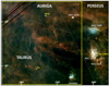 |
Fig. 1. Map of the dust distribution in the Taurus, Auriga, Perseus star forming complexes obtained by the Far Infrared Surveyor on board the AKARI satellite. The location of the main young associations is indicated as well as that of T Tau and AB Aur, two prominent pre-main sequence stars in the region. The yellow frame marks the area surveyed by GALEX and searched for young stars by GdC2015. |
The release of the Gaia data release 2 (DR2) catalog (Gaia Collaboration 2018) enabled for the first time an unbiased search for WTTSs in the region based on the kinematical properties of the stars. The Gaia survey is magnitude limited to G ≃ 21 and is therefore sensitive to the low-mass stellar population (late M types) in the TAMC, which is located at ∼140 pc. Galli et al. (2019) generated a compilation of all the possible T Tauri stars (TTSs) in the region including both confirmed spectroscopic sources and possible candidates, which were identified by the surveys carried out with the Spitzer infrared telescope (Luhman et al. 2010), the Sloan Digital Sky Survey, and the 2-Microns All Sky Survey (Luhman et al. 2017). Using a Hierarchical Mode Association Clustering (HMAC) algorithm, these authors classified these sources into 21 distinct kinematical groups. A recent re-evaluation based on Gaia DR3 (Gaia Collaboration 2023) data resulted in a grand total of 532 adopted members distributed over 13 kinematical groups (Luhman 2023). This kinematical search does not provide a complete census of the young stars in the region because young stars with peculiar proper motions, such as stars ejected in close encounters or stars in multiple systems, will be rejected as outliers by the classification algorithms. Also, no information on their youth or evolutionary state can be obtained in this manner. An additional problem is the scarce and uncertain information provided by Gaia DR3 on the radial velocity of these stars, which makes accurate determination of the three components of the LSR velocity (U, V, W) difficult for a large fraction of the sources.
The most common and successful ways to search for WTTSs in molecular clouds are based on their strong magnetic activity, which results in an enhancement of the atmospheric flux: coronal emission at X-ray wavelengths, the radiation from the transition region at ultraviolet (UV) wavelengths, and the chromospheric radiation measurable at UV but also at optical wavelengths. The first catalogs of TTSs were built from stars displaying enhanced chromospheric emission at the Hα line (see e.g., Herbig & Kameswara Rao 1972). Many WTTS candidates were identified in the TAMC from the ROSAT all-sky X-ray survey (Neuhaeuser et al. 1995), and subsequent observations (especially of the Li I absorption) proved that many were indeed WTTSs. The release of the “all sky UV survey” carried out by the Galaxy Evolution Explorer (GALEX) enabled the search for TTSs by their UV excess; a list of 63 new TTS candidates was elaborated by comparing the UV color and the IR color excesses in the TAMC (Gómez de Castro et al. 2015, hereafter GdC2015). Gaia was launched in December 2013 and its subsequent data releases came much later than the publication of this list; therefore, neither parallax nor kinematical information was available at the time to narrow down this large list of candidates. The purpose of the present research is to carry out such an analysis in order to identify the bona fide TTSs in the sample. For this purpose, we use the Gaia DR3 parallax and kinematical information as well as spectra from the spectroscopic survey carried out by the Large Sky Area Multi-Object Fiber Spectroscopic Telescope (LAMOST) when available in order to determine the spectral type and the Li I equivalent width.
This article is structured as follows. In Sect. 2, the characteristics of the GdC2015 sources are described. Sources with Gaia DR3 parallaxes incompatible with TAMC membership are disregarded, reducing the working sample of viable candidates to 13 sources. In Sect. 3, the membership probability of these candidates is evaluated using Gaia DR3 data. In the process, a list of trusted TTSs in the TAMC for kinematical studies is produced; this compilation is significantly shorter than that produced by Luhman (2023). In Sect. 4, we present an analysis of LAMOST spectra; two new accreting late M-type stars are identified in the GdC2015 sample. Finally, a short discussion (Sect. 5) on the radial velocity distribution of the TTSs and the coupling with the molecular gas is included. We provide a short summary of our findings in Sect. 6. Technicalities concerning the error analysis of the samples are compiled in the appendix to facilitate a comprehensive reading of the work.
2. UV candidates to T Tauri stars in the Taurus-Auriga region
The GALEX All Sky Survey (AIS; Martin et al. 2005) provided the first unbiased view of the TAMC at UV wavelengths. Though the area was not mapped completely, because of GALEX sensitivity constraints, 380 sq. deg. in the sky (equivalent to 197 GALEX fields) were imaged and as many as ∼163 000 UV sources were detected in the near ultraviolet (NUV) band (see GdC2015). Through a comparison of UV and IR colours, 63 new candidate TTSs were identified; their location is shown in the top panel of Fig. 2 and their UV-IR colours in the bottom panel.
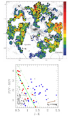 |
Fig. 2. Candidate TTSs in the TAMC from GdC2015. Top panel: location of the TTSs and candidates on the sky overlaid on the density of GALEX NUV sources, in galactic coordinates; stellar densities are color coded. The density of molecular gas is outlined from the 2MASS extinction map by Lombardi et al. (2010). Bottom panel: color–color diagram used for the selection of the TTSs candidates in GdC2015. Candidates are marked with black crosses, and known CTTSs and WTTSs from the qualification sample are represented by blue squares and red circles, respectively. The regression line marking the location of the WTTSs in the diagram is plotted (solid green line) as well as the uncertainty band from the fit (dashed green lines); most of the TTS candidates to be analyzed in this work are within this strip. |
These 63 sources were selected using a qualification sample of TTSs that was generated from two sets of sources: [1] the 31 known TTSs detected in the GALEX AIS survey of the TAMC and [2] the 21 TTSs observed with the International Ultraviolet Explorer (IUE) in the low dispersion mode with high-signal-to-noise ratio spectra (see Table 1 in GdC2015); synthetic GALEX photometry was calculated from the IUE spectra for these sources using the conversion proposed by Morrissey et al. (2007). 2MASS photometry was available for all the sources in the qualification sample. All these stars are marked with blue squares (if classical TTSs (CTTSs) and red circles (if weak-line TTSs (WTTSs)) in the bottom panel of Fig. 2. The 63 candidates to be evaluated in this work appear as crosses in the plot.
We note that the WTTSs define a clear regression line with the hardest UV colours being observed in the sources displaying the smallest J − K color. However, CTTSs are scattered in the diagram. Most of the candidates studied in this work were identified in the WTTSs strip (see Fig. 2, bottom panel) close to the location of reddened massive cool stars and many are located close to the Galactic plane (see Fig. 2, top panel). Therefore, further observables, such as distance or kinematics, are needed to confirm the PMS nature of these sources. We searched for and found Gaia DR3 counterparts for all candidates using a 2 arcsec search radius, employing the cross match services provided by the Centre de Données Stellaires (CDS).
In Fig. 3, we display the projected location on the plane of the sky of all sources within 1200 pc. Only 13 among them have parallaxes compatible with TAMC membership; that is, 5 mas−9 mas, according to Roccatagliata et al. (2020). Seven among them are concentrated in the north of the region, close to the Galactic plane, but are separated in two distance groups at ∼110 pc and ∼160 pc.
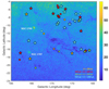 |
Fig. 3. Density of Gaia sources in the TAMC. The densities are color coded in stars per 6 arcmin2 (see lateral bar). The shadow produced by the TAMC filaments over the stellar background is readily identified. The two over-dense regions are: the open cluster NGC 1747 located at 550 pc and the asterism or apparent concentration of stars (Cantat-Gaudin & Anders 2020) named NGC 1746. The locations of the GdC2015 candidates with Gaia counterparts within 1200 pc are marked with circles and asterisks, and are color coded by distance. Asterisks represent sources with high-quality Gaia measurements (RUWE ≤ 1.4) and circles denote sources with RUWE larger than this threshold. |
3. Kinematical properties of the candidates
In addition to distance, stellar kinematics needs to be analyzed. This was done in two steps. First, we studied the kinematics of known and trusted TTSs in the TAMC with high-quality Gaia measurements1. We identified kinematical groups within this sample using the k-means++ algorithm and then evaluated the probability for each of the 13 candidates to be a kinematical member. Only trusted PMS sources with high-quality astrometric data are considered for this qualification sample. The Gaia Data Processing and Analysis Consortium states that a value of the renormalized unit weight error (RUWE) ≤ 1.4 is indicative of a good astrometric solution. Therefore, only Gaia observations with RUWE ≤ 1.4 were considered for the qualification of the kinematics of the TTSs in the TAMC. As an aside, we note that, according to Stassun & Torres (2021), RUWE values even slightly above 1.0 may signal unresolved binaries in Gaia data.
3.1. Kinematics of known TTSs in the TAMC
The initial sample of trustworthy TTSs in the TAMC was taken from Joncour et al. (2017); more recent catalogs are available, such as Galli et al. (2019) and Luhman (2023), but together with bona fide TTSs these catalogs include candidate TTSs from various surveys. The Joncour et al. (2017) compilation includes 338 sources and is mainly based on the mid-infrared (MIR) survey of the TAMC that was carried out with the Spitzer telescope to perform a census of the disc population in the region. This census was completed with Hα data for the few TTSs that were not detected (Luhman et al. 2010). Only 274 sources of the Joncour et al. (2017) catalogue have a Gaia DR3 counterpart and only 170 have measurements with RUWE ≤ 1.4.
Thus, our initial qualification sample consisted of these 170 TTS with high-quality astrometric measurements; however, after cross-checking Gaia parallaxes, three sources were found to not belong to the TAMC and were therefore discarded (see Table 1). The final qualification sample consists of 92 CTTSs and 75 WTTSs (see Table 2).
Sources misclassified as TTSs in the TAMC.
Qualification sample for the kinematics of the TTSs in the TAMC.
We converted Gaia proper motions in the ICRS system into the Galactic system using the procedure described in the Gaia EDR3 documentation2. In Fig. 4, these proper motions are overlaid on the map obtained by the Plank mission of the area where the distribution of the warm dust and the orientation of the magnetic field are shown (Planck Collaboration XLII 2016). The motion of the TTSs is very coherent, as expected in a young association that still keeps memory of the motion of the parent molecular cloud; the young gravitationally bound open cluster contains hundreds of members of similar age and composition; however, the kinematical memory of this common origin will be lost over time due to the interaction with the large-scale gravitational field of the Galaxy. As pointed out back in the early 1990s (Gomez de Castro & Pudritz 1992) the TTSs move roughly perpendicularly to the direction of the magnetic field traced by the polarization of the dust.
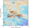 |
Fig. 4. Proper motions (velocity projected in the plane of the sky) of the known TTSs in the TAMC with high-quality astrometric measurements (RUWE < 1.4). CTTSs and WTTSs are represented with blue and red arrows, respectively. We note that the motion of the stars is not parallel to the filaments and is approximately perpendicular to the direction of the magnetic field. |
There are mild differences between WTTSs and CTTSs. This is best shown by the μb/μl ratio (see Figs. 4 and 5); while CTTSs have a single-peak distribution with a smooth tail to small ratios, the WTTSs display a double-peaked distribution. As CTTSs are younger stars, it is expected that they are better coupled to the gas and retain a common kinematics. This effect is also observed in the spatial distribution of the accreting TTSs and the WTTSs; CTTSs are located close to the molecular cloud, while WTTSs are more sparsely distributed (Luhman et al. 2010). Two outliers are detected: the CTTS, LkHα 332 (2MASS J04420777+2523118) and the WTTS 2MASS J04555288+3006523; LkHα 332 is located 11.3 arcsec from V1000 Tau, another TTS.
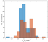 |
Fig. 5. Histogram of the distribution of the ratio μb/μlcos(b) obtained for the known CTTSs (blue) and WTTSs (red) in the TMC. |
3.1.1. k-cluster analysis
The TAMC occupies a large area in the sky and several kinematic groups have been identified within the association (see e.g., Galli et al. 2019; Luhman 2023). In the present work, we used the k-means++ clustering algorithm to determine which groups of stars in our qualification sample could be kinematically related. Given their young age, kinematically coherent sources may have been born out of the same gas cloudlet within the TAMC. k-means++ is an unsupervised machine-learning algorithm that performs a centroid-based analysis using iterative refinement (Lloyd 2006; Arthur & Vassilvitskii 2007). In our case, we carried out a multiparametric analysis that included both positional information (parallax) and kinematic information (the projections of the proper motion along the Galactic coordinates); that is, our data set has three parameters. The k-means++ algorithm is not based on density, as in DBSCAN or OPTICS, but is partitional, and so every object in the sample is assigned to one cluster only. This algorithm implicitly assumes that clusters are convex and isotropic and it performs best when applied to a mixture of Gaussian distributions with the same variances but perhaps different means. This mathematical precondition is a good match to the physical context of the TAMC sample when parallaxes and proper motions are considered. As our analysis does not include the coordinates of the sources, but parallaxes and proper motions instead, the actual distributions of the data are rather isotropic and normally distributed.
We generated a three-dimensional vector for each of the 167 TTSs (92 CTTSs and 75 WTTSs). An initial set of k points (centroids) was defined in this three-dimensional space and k clusters were created by associating every vector with the nearest centroid. In a second step, a new centroid was computed for each cluster by calculating the mean among the vectors. Later, the association of each vector to a given cluster was re-evaluated for the new centroid. The process was repeated until convergence was reached.
Here, we used the k-means++ algorithm as implemented by the Python library Scikit-learn (Pedregosa et al. 2011). Before applying the k-means++ algorithm, we scaled the data set using Z-score normalization: we found the mean and standard deviation for each set of variables used in the analysis, subtracted the relevant mean from each value, and then divided by its corresponding standard deviation. Although the variables may originally have different variances, Z-score normalization standardizes variances and avoids placing more weight on variables with smaller variance when applying k-means++. Distance assignment between the data points in our sample assumed a Euclidean metric (other metrics gave consistent results) and we used the elbow method to determine the optimal value of clusters, k, that minimized the sum of the distances of all data points to their respective cluster centres. Test analyses using OPTICS on the same data set led to similar results.
This procedure was applied to the list of bona fide TTSs (Table 2); but in order to take into account the associated uncertainties and their correlations, we generated 104 instances of the sample as explained in Appendix A and for each synthetic instance, we determined the clusters through the k-means++ algorithm. In almost all the cases, our clustering analysis produced two statistically significant clusters, which are represented in Fig. 6. Sources in the first group are located at an average distance of 160 pc, while those in the second group are found at 130 pc. This clean classification in two groups differs from the results of the previous works by Galli et al. (2019) and Luhman (2023). Galli et al. (2019) used Hierarchical Association Clustering Mode (HACM), which is a nonparametric statistical approach used for clustering analysis. HACM finds the modes of a kernel-based estimate of the density of points in the working space and groups the data points associated with the same modes into one cluster with arbitrary shape. Clustering by mode identification requires only the space and the bandwidth of the kernel to be defined. In particular, Galli et al. (2019) made use of a five-dimensional space consisting in the equatorial coordinates of the sources, their proper motions in equatorial coordinates, and the parallax (α, δ, μδ, μαcosδ, π). The algorithm identifies 21 clusters hierarchically linked in the dendrogram, with only 4 of them having more than ten sources. This result is natural, because the coordinates are taken into account and the stellar population is sparsely distributed in the TAMC; therefore, stars with similar proper motions and parallaxes located in different areas are identified as independent groups. Luhman (2023) followed a different approach. These authors analyzed Gaia astrometry in terms of proper-motion offsets, which are defined as the differences between the observed proper motion of the star and the motion expected at the celestial coordinates and parallactic distance of the star for a specified space velocity. This procedure is set to minimize the projection effects given the large extent of the TAMC and the offsets are calculated with respect to the expected LSR velocity given in terms of the velocity vector (U, V, W)=(−16, −12, −9) km s−1, which according to Luhman (2018) approximates the median velocity of Taurus members. Luhman (2023) identified nine groups in this manner (see their Fig. 1 and Table 6). These groups do not coincide with those found by Galli et al. (2019), but some of the levels in the hierarchy defined by Galli et al. (2019) contain some of these groups. In our work, the classification is made with a k-means++ clustering algorithm, which does not provide a hierarchical classification, or a dendrogram suitable for comparison with Galli et al. (2019). Moreover, the analysis in Sect. 3.1, as well as previous works (Gomez de Castro & Pudritz 1992), show that galactic coordinates are better suited for the kinematical analysis of the region (see Fig. 4). Proper motions are converted from equatorial to galactic coordinates and the cluster analysis is carried in a three-dimensional space, including these proper motions and the parallax (μb, μlcosb, π). The number of groups identified by the algorithm is reduced to two (groups 0 and 1), with a clear difference between them in both proper-motion space and distance. Groups L1544 and L1517 in Luhman (2023) belong to group 0 and 1 in this work, respectively. However, the many groups identified by Luhman (2023) in the center of the TAMC belong to one of the two underlying groups identified in this work. Our method does not assume a common LSR velocity for the full TAMC, as in Luhman (2023), and does not require knowledge of the radial velocity of the stars in order to evaluate the differences in the (U, V, W), because there are very few sources with accurate determinations of the radial velocity (see Galli et al. 2019). We simply use high-quality data from Gaia DR3 and the properties of the TAMC analyzed in this work, in order to choose optimal dynamical tracers for the classification. This strategy has proven to be very efficient in the description of the region.
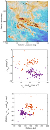 |
Fig. 6. Location of the two groups identified by the decision tree algorithm. Top: source locations. Middle: proper motions of the sources in Galactic coordinates. Bottom: inclination of the proper motion with respect to the Galactic plane versus distance. The two groups are identified by orange squares (group 0) and violet circles (group 1). |
3.2. Kinematics of the TTS candidates and membership probability
Above, we discuss the kinematics in the TAMC based on the sample of 167 “bona fide” TTSs. In this section, we use the kinematic classification – performed in Sect. 3.1 – to assign a membership probability (to each of the two groups) to each of the 13 TTS candidates. To this end, we built a logistic regression model using the Scikit-learn package (Pedregosa et al. 2011). A detailed explanation of this method, with an application to astrophysics, is provided in Beitia-Antero et al. (2018); in the present work, we only provide a simple explanation of the methodology as a guide to the reader for our particular case.
We work with a qualification sample of N = 167 stars (the “bona fide” TTS), which are classified into two groups based on their values of (μl*, μb, π) as explained in the previous section. This classification therefore depends on three features and is binary (groups k = {1, 0}). In this case, the logistic regression model gives the probability that a given star xi belongs to Group 1, and the probability of belonging to Group 0 is the complement to this latter:
 (1)
(1)
where βm are the logistic regression parameters fitted using the qualification sample; these have a median value of β0 = 17.052, β1 = −0.085, β2 = 0.616, β3 = −1.575 (see Appendix B for more details on how these parameters were computed, taking into account the associated errors on proper motions and parallax). We analyzed the confusion matrix and only one star is misclassified. This choice of parameters (proper motions in galactic coordinates and parallax) therefore leads to good separation of the groups.
Having trained the logistic regression model, we applied it to the sample of TTS candidates, and following the methodology explained in Appendix B, we took into account the errors in the measurements and computed a median probability of belonging to each of the two groups; these probabilities are shown in Table 3. The locations of the candidates in the proper motion–distance diagram are shown in Fig. 7. Only sources No. 3 (J04423721+3401492) and No. 12 (V600 Aur) display properties very different from those of the qualification sample. We want to highlight that we even computed membership probability for those sources with astrometric measurements of moderate quality, namely J04290082+3152597 (RUWE: 1.413), J05000310+3001074 (RUWE: 1.615), and J05005485+3229168 (RUWE: 1.773), and poor quality: J04455129+1555496 (RUWE: 4.6815).
Classification of the 13 TTS candidates after applying the logistic regression model with variables (π, μlgalcosbgal, μlgal).
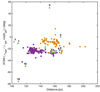 |
Fig. 7. As in the bottom panel of Fig. 6. The locations of the 13 candidate TTSs examined in this work are indicated and labeled according to their entry in Table 3. The candidates are marked according to their RUWE value: green diamonds (RUWE ≤ 1.4) and black dartboards (RUWE > 1.4). |
4. Spectral information on the candidates
In addition to the kinematical information, Gaia DR3 provides data on the effective temperature, surface gravity, and metallicity for 7 of the 13 candidate sources (see Table 4). These data are also indicated in the table and are compatible with the candidates being late-type stars, as expected for the TAMC stellar population.
Stellar properties.
A peculiar source is HO Aur. The metallicity derived by Gaia for this source is very low (−3.9707), and given the high quality of the measurements (RUWE < 1.4), we feel inclined to rely on the data provided by the mission and tentatively identify HO Aur as a Population II field star.
LAMOST spectra are available for a few sources and are compatible with the effective temperatures derived by Gaia. In particular, the spectra of J04510713+1708468 and J05240794+2542438 are compatible with late M spectral type and display strong TiO bands. We downloaded the spectra from the Vizier server and measured the TiO-5 index (Cruz & Reid 2002) for these sources, obtaining values of 1.28 and 0.85, respectively, which confirms their M-type classification. The spectra also display a strong Na I absorption feature at 8183/8199 Å (see Fig. 8), which is gravity sensitive (Martín et al. 2010). Unfortunately, the spectral resolution is too low to cross-check the effective gravity determined by Gaia for these sources. The spectra also show Li I absorption at 6708 Å but again, equivalent widths are very uncertain and it is therefore difficult to provide an age estimate of the sources.
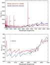 |
Fig. 8. LAMOST spectrum of the two newly identified accreting brown dwarfs in the TAMC. Top: LAMOST spectrum; the Balmer series and the TiO bands are readily identified. Bottom: zoom onto the Li I feature. |
The most noticeable characteristics of the spectra of these stars are the prominent emission lines, in particular the Balmer series and the Ca II doublet (see Fig. 8). This indicates that the two M dwarfs are young and possibly accreting (see Basri 2000, and references therein). This is consistent with the method used by GdC2015 to search for TTSs candidates, where sources were selected based on their UV excess: 2MASS J04510713+1708468 has FUV − NUV = 1 and J − K = 0.9, and 2MASS J05240794+2542438 has FUV − NUV = 1.4 and J − K = 0.97.
HD 281691 is a G8 star located in front of the TAMC at a distance of 108.7 pc according to the Gaia parallax, and its proper motions are significantly different from those of the TTSs in the system. HD 281691 has a nearby companion located at a projected distance of 6.78 arcsec (738 AU; Janson et al. 2013) and is often included in surveys for debris disk (Meshkat et al. 2017). The IR excess from the disk and the UV emission from the active star resulted in its detection by the GdC2015 survey.
HD 30171 (J04455129+1555496) was detected as a TTS candidate in the GdC2015 survey and has been known to be a WTTS since the early searches for Li I absorption of the X-ray sources detected by the ROSAT satellite in TAMC (Wichmann et al. 2000). As such, it is included in the catalogue used for qualification of the TTS sample (Joncour et al. 2017) and is a clear member of Group 2.
V600 Aur is an active X-ray source that was included in the sample studied by Xing (2010) for the determination of the Li I equivalent width (see Table 1 in the article, [LH98] 173). Its rapid rotation period (2.201 days) and high Li I abundance support both its PMS nature and TAMC membership. We note that, though its kinematics deviates apparently from that of the TAMC members, this may be caused by the low quality of the Gaia measurements (RUWE = 3.529).
J04590305+3003004 and J05000310+3001074 are included in the Catalogue of Stars in the Northern Milky Way Having Hα in Emission (Kohoutek & Wehmeyer 1999) and display infrared excess emission (Luhman 2023). Recently, J04590305+3003004 was reported as a 8.8 Myr old dipper star, a subgroup among the young stellar objects whose members exhibit dimming variability in their light curves (drops in brightness by 10%−50%), which is attributed to the occultation of the star by the circumstellar disk material (Capistrant et al. 2022).
Little or no information is available for J04290082+3152597, J04423721+3401492, J04595003+3049082, J05005485+3229168, and J05050770+2923477. According to the work presented here, two of these are very good candidate members of the sparse young stellar population of the TAMC. However, the kinematics of J04423721+3401492 differs significantly from that of the TAMC members and the quality of the Gaia measurements is quite good (RUWE = 1.482).
In summary, 3 of the 13 candidates identified in the GdC2015 survey are known PMS stars, namely HD 30171, V600 Aur, and J04590305+3003004. Another two are not TTSs associated with the TAMC; HD 281691 is a field G8-type star located in front of the TAMC with a nearby companion at a projected distance of 738 AU, and HO Aur has too low a metallicity to belong to the TAMC. The remaining sources (excluding J04423721+3401492) are very reliable candidates, and two of them in particular have been confirmed as new late-type TTSs based on their LAMOST spectrum: J04510713+1708468 and J05240794+2542438.
5. Discussion: Dynamical coupling between the TAMC and the TTSs in the region
The radial velocity of the TTSs also provides important information that can be used to determine the coupling between the molecular gas in the TAMC and the young stellar population (see e.g., Gomez de Castro & Pudritz 1992). This determination is relevant for two purposes. First, it indicates the degree of dynamical relaxation of the young stellar association. Also, if the coupling is strong, this information can be used to estimate the motion of the molecular gas in the plane of the sky, which would be unfeasible otherwise; if the dynamical coupling between the gas and the stars is strong (if the radial velocities are similar), then the motion of the clouds in the plane of the sky can be inferred from the stellar motion and the 3D velocity vector of the molecular gas can be restored.
There have been several attempts to examine this coupling; in particular by Galli et al. (2019) based on Gaia DR2 data. These latter authors selected several TTSs (28) and compared their radial velocity with that of the molecular gas in the nearest area within the complex (see Fig. 15 in Galli et al. 2019). There is a well-known velocity gradient in the TAMC that is observed in the 12CO and 13CO maps (Goldsmith et al. 2008; Narayanan et al. 2008); the radial (VLSR) velocity decreases from 8.5 to 5.5 km s−1 roughly as Galactic longitude increases (see Figs. 7–16 in Narayanan et al. 2008). Galli et al. (2019) attempted to look for traces of this gradient in the stellar radial velocity, with uncertain results. In their work, they selected the TTSs with good radial velocity measurements from Gaia DR2 and extracted from the 13CO data cubes the velocity of the nearby (in projection) molecular gas (the beam size of the radio maps is 45″ and the Nyquist-samplex pixel ∼20″). They found that stars near L1495, B213, and B216 (which are at lgal ∼ 170°) have larger VLSR than stars at L1536 (lgal ∼ 175°), but the correlation is not good beyond these two extreme groups. Moreover, the uncertainties of the 13CO VLSR measurements are high given the large broadening of the 13CO profiles and the extent of the area within the beam. In summary, though the attempt is to be commended, the results are inconclusive.
A simpler, statistical approach may help to examine the star–gas coupling. There are about 6.2 million stars with galactic coordinates (lgal ∈ [164° ,185° ], bgal ∈ [ − 24° , − 4° ]) in the Gaia DR3 survey. This number reduces to 697 990 if only sources with accurate radial velocity (relative error < 10%) are included. Among them, only 20 806 are located at a distance compatible with TAMC membership. We evaluated the radial velocity distribution (VLSR) for these field stars and compared it with that obtained for the TTSs with high-quality Gaia DR3 radial velocity measurements (66 TTSs, of which 40 are WTTSs and 26 are CTTSs). The velocity distribution of the field stars in the area is very broad with a slight asymmetry towards blueward-shifted velocities; however, the velocity distribution of the TTSs (both WTTSs and CTTSs) peaks at redward-shifted velocities of ∼2.5 km s−1 (see Fig. 9). The Kolmogorov–Smirnov test rejects the null hypothesis (both distributions are the same); the p-value is 1.32 × 10⁻¹². Therefore, as expected, the TTSs also differ from field stars in radial velocity. The relevant issue for the sake of this discussion is that the peak frequency of the velocity of TTSs is smaller than the VLSR of the TAMC, and therefore the TTSs as a whole seem to be already dynamically decoupled from the cloud.
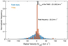 |
Fig. 9. Histogram of the frequencies of the distribution of stars in the TAMC field in terms of VLSR. The distribution of field stars is compared with that of the bona fide TTSs. |
Unfortunately, the statistics are too poor to look for differences between CTTSs and WTTSs. In spite of the apparent slight bias of the CTTSs towards a higher VLSR as suggested by the results shown in Fig. 10, the Kolmogorov–Smirnov test clearly indicates that the CTTS and WTTS distributions are independent samples of the same underlying distribution with a p-value of 0.998.
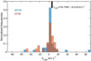 |
Fig. 10. Histogram of the frequencies of the distribution of TTS stars in terms of VLSR. The distribution of the CTTSs is compared with that of the WTTSs. |
6. Summary
In this work, Gaia DR3 astrometric data were used to review the list of candidate TTSs selected by GdC2015 on the basis of their UV and IR colours. From the initial compilation of 63 sources, we find that only 10 (16%) are reliable members (shared kinematics and location with well-known members of the association). Most of these sources are located at low galactic latitudes, in the Auriga-Perseus area. Gaia spectroscopic information shows that one of the candidates in the GdC2015 list, HO Aur, is a very low-metallicity population II star and cannot be a member of this young association. The rest of the sources are very likely TTSs; in particular, we identify two of them as accreting late-type dwarfs based on their LAMOST spectra: 2MASS J04510713+1708468 and 2MASS J05240794+2542438.
This work also provided some additional results. First, it provides a clean, reliable list of TTSs for astrometric studies. In addition, the analysis of the radial velocity (VLSR) of the TTSs in comparison to those of the field stars and the molecular cloud shows that the association has clearly distinct kinematics and that the TTSs are no longer coupled to the molecular gas in the TAMC. As the sample is dominated by WTTSs, this suggests that the decoupling is already significant 10 − 100 Myr after star formation begun.
Acknowledgments
This work has been partially financed by the Ministry of Science and Innovation through grants: ESP2017-87813-R and PID2020-116726RB-I00. This research has made use of the SIMBAD database, operated at CDS, Strasbourg, France and the computational facilities of the Joint Center for Ultraviolet Astronomy in the campus of the Universidad Complutense de Madrid. L.B.-A. acknowledges the receipt of a Margarita Salas postdoctoral fellowship from Universidad Complutense de Madrid (CT31/21), funded by the “Ministerio de Universidades” with Next Generation EU funds. This work has made use of data from the European Space Agency (ESA) mission Gaia (https://www.cosmos.esa.int/gaia), processed by the Gaia Data Processing and Analysis Consortium (DPAC, https://www.cosmos.esa.int/web/gaia/dpac/consortium). Funding for the DPAC has been provided by national institutions, in particular the institutions participating in the Gaia Multilateral Agreement.
References
- Arthur, D., & Vassilvitskii, S. 2007, Proceedings of the Eighteenth Annual ACM-SIAM Symposium on Discrete Algorithms (Philadelphia: Society for Industrial and Applied Mathematics), 1027 [Google Scholar]
- Basri, G. 2000, ARA&A, 38, 485 [NASA ADS] [CrossRef] [Google Scholar]
- Beitia-Antero, L., Yáñez, J., & de Castro, A. I. G. 2018, Exp. Astron., 45, 379 [NASA ADS] [CrossRef] [Google Scholar]
- Cantat-Gaudin, T., & Anders, F. 2020, A&A, 633, A99 [NASA ADS] [CrossRef] [EDP Sciences] [Google Scholar]
- Capistrant, B. K., Soares-Furtado, M., Vanderburg, A., et al. 2022, ApJS, 263, 14 [NASA ADS] [CrossRef] [Google Scholar]
- Cruz, K. L., & Reid, I. N. 2002, AJ, 123, 2828 [NASA ADS] [CrossRef] [Google Scholar]
- Gaia Collaboration (Brown, A. G. A., et al.) 2018, A&A, 616, A1 [NASA ADS] [CrossRef] [EDP Sciences] [Google Scholar]
- Gaia Collaboration (Vallenari, A., et al.) 2023, A&A, 674, A1 [NASA ADS] [CrossRef] [EDP Sciences] [Google Scholar]
- Galli, P. A. B., Loinard, L., Bouy, H., et al. 2019, A&A, 630, A137 [NASA ADS] [CrossRef] [EDP Sciences] [Google Scholar]
- Garufi, A., Podio, L., Codella, C., et al. 2021, A&A, 645, A145 [EDP Sciences] [Google Scholar]
- Goldsmith, P. F., Heyer, M., Narayanan, G., et al. 2008, ApJ, 680, 428 [Google Scholar]
- Gomez de Castro, A., & Pudritz, R. E. 1992, ApJ, 395, 501 [CrossRef] [Google Scholar]
- Gómez de Castro, A. I., Lopez-Santiago, J., López-Martínez, F., et al. 2015, ApJS, 216, 26 [CrossRef] [Google Scholar]
- Herbig, G. H., & Kameswara Rao, N. 1972, ApJ, 174, 401 [NASA ADS] [CrossRef] [Google Scholar]
- Janson, M., Brandt, T. D., Moro-Martín, A., et al. 2013, ApJ, 773, 73 [Google Scholar]
- Joncour, I., Duchêne, G., & Moraux, E. 2017, A&A, 599, A14 [NASA ADS] [CrossRef] [EDP Sciences] [Google Scholar]
- Kohoutek, L., & Wehmeyer, R. 1999, A&AS, 134, 255 [NASA ADS] [CrossRef] [EDP Sciences] [Google Scholar]
- Lloyd, S. 2006, IEEE Trans. Inf. Theor., 28, 129 [Google Scholar]
- Lombardi, M., Lada, C. J., & Alves, J. 2010, A&A, 512, A67 [NASA ADS] [CrossRef] [EDP Sciences] [Google Scholar]
- Long, F., Herczeg, G. J., Harsono, D., et al. 2019, ApJ, 882, 49 [Google Scholar]
- Luhman, K. L. 2018, AJ, 156, 271 [Google Scholar]
- Luhman, K. L. 2023, AJ, 165, 37 [NASA ADS] [CrossRef] [Google Scholar]
- Luhman, K. L., Allen, P. R., Espaillat, C., Hartmann, L., & Calvet, N. 2010, ApJS, 186, 111 [Google Scholar]
- Luhman, K. L., Mamajek, E. E., Shukla, S. J., & Loutrel, N. P. 2017, AJ, 153, 46 [Google Scholar]
- Martin, D. C., Fanson, J., Schiminovich, D., et al. 2005, ApJ, 619, L1 [Google Scholar]
- Martín, E. L., Phan-Bao, N., Bessell, M., et al. 2010, A&A, 517, A53 [Google Scholar]
- Meshkat, T., Mawet, D., Bryan, M. L., et al. 2017, AJ, 154, 245 [Google Scholar]
- Morrissey, P., Conrow, T., Barlow, T. A., et al. 2007, ApJS, 173, 682 [Google Scholar]
- Narayanan, G., Heyer, M. H., Brunt, C., et al. 2008, ApJS, 177, 341 [NASA ADS] [CrossRef] [Google Scholar]
- Neuhaeuser, R., Sterzik, M. F., Schmitt, J. H. M. M., Wichmann, R., & Krautter, J. 1995, A&A, 297, 391 [NASA ADS] [Google Scholar]
- Pedregosa, F., Varoquaux, G., Gramfort, A., et al. 2011, J. Mach. Learn. Res., 12, 2825 [Google Scholar]
- Planck Collaboration XLII. 2016, A&A, 596, A103 [NASA ADS] [CrossRef] [EDP Sciences] [Google Scholar]
- Roccatagliata, V., Franciosini, E., Sacco, G. G., Randich, S., & Sicilia-Aguilar, A. 2020, A&A, 638, A85 [NASA ADS] [CrossRef] [EDP Sciences] [Google Scholar]
- Stassun, K. G., & Torres, G. 2021, ApJ, 907, L33 [NASA ADS] [CrossRef] [Google Scholar]
- Ungerechts, H., & Thaddeus, P. 1987, ApJS, 63, 645 [Google Scholar]
- Wichmann, R., Torres, G., Melo, C. H. F., et al. 2000, A&A, 359, 181 [NASA ADS] [Google Scholar]
- Xing, L. F. 2010, ApJ, 723, 1542 [NASA ADS] [CrossRef] [Google Scholar]
Appendix A: Impact of uncertainties on our clusterings analysis
In order to account for the data uncertainties, we used a Monte Carlo sampling technique to generate 104 synthetic datasets. For each one, we applied the k-means++ algorithm, keeping track of the number of groups generated and the positions of the centroids (the nearest neighbor was used as a proxy to obtain physical coordinates). Therefore, for each source in our list of bona fide TTSs, we generated 104 realizations of its astrometric parameters. Gaia DR3 provides the correlations between each pair of astrometric parameters. Given two parameters, x and y, with standard deviations σx and σy, their respective covariance and correlation coefficients, σxy and ρxy, can be written as σxy = ρxy σx σy. If C is the covariance matrix at a given epoch associated with the astrometric solution that is symmetric and positive-semidefinite, then C = AAT where A is a lower triangular matrix with real and positive diagonal elements, and AT is the transposition of A. In the particular case studied here, these matrices are 5 × 5. If the elements of C are written as cij = ρij σi σj and those of A as aij, where those are the entries in the i-th row and j-th column, and if r is a vector made of univariate Gaussian random numbers (components ri with i = 1, 5), the required multivariate Gaussian random samples are given by the expressions:
 (A.1)
(A.1)
where α, δ, π, μα, and μδ are the values of right ascension, declination, absolute stellar parallax, and proper motions in right ascension and declination directions provided by Gaia DR3 and the aij coefficients are given by:
 (A.2)
(A.2)
where σα, σδ, σπ, σμα, and σμδ are the standard errors in right ascension, declination, parallax, and proper motions from Gaia DR3, and ρα δ, ρα π, ρα μα, ρα μδ, ρδ π, ρδ μα, ρδ μδ, ρπ μα, ρπ μδ, and ρμα μδ their respective correlation coefficients, also from Gaia DR3. For each πc, we computed the value of the distance by applying the usual relationship, dc = 1/πc.
For each set of synthetic sources statistically compatible with the qualification sample, we computed the proper motions along the Galactic coordinates as pointed out above and used their values together with the parallaxes to apply the k-means++ algorithm. The resulting centroids are shown in Fig. A.1 in red.
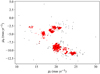 |
Fig. A.1. Effect of the uncertainties on the clustering analysis. Results in physical parameters. In black we have the sources and in red the 104 centroids. |
Appendix B: Fitting the logistic regression model with errors
From a mathematical point of view, the logistic regression model is trained on a set of qualification sources with well-defined groups, where all the values are considered to be free of errors. However, the proper motions and parallax of our training sample of bona fide TTSs have inherent errors and depend on each other – the parameters are correlated. In order to take this constraint into account, we produced a set of 104 mock realizations of the sample using the covariance matrix for generating random samples of (μα*, μδ, π), which we then converted into proper motions in Galactic coordinates as explained in the Gaia documentation3. As a result, we obtained a distribution for each value of the logistic regression model (βm, m = 0, 1, 2, 3) as shown in Fig. B.1. In these plots we have included the median value for each coefficient in black, which is taken as the best-fit value, as well as the results if we fit the original sample without taking the errors into account.
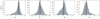 |
Fig. B.1. Final distributions for the logistic regression coefficients after 104 Monte Carlo realizations. The solid black line corresponds to the median value adopted as the best fit, while the red dashed line corresponds to the value obtained from the fit of the original variables without taking errors into account. |
For the classification of the TTS candidates, we performed an analogous Monte Carlo analysis and again generated 104 samples, taking into account the errors, and for each realization we assigned a membership probability. The values given in the main text are the median values of the probabilities of the 104 random samples.
All Tables
Classification of the 13 TTS candidates after applying the logistic regression model with variables (π, μlgalcosbgal, μlgal).
All Figures
|
Fig. 1. Map of the dust distribution in the Taurus, Auriga, Perseus star forming complexes obtained by the Far Infrared Surveyor on board the AKARI satellite. The location of the main young associations is indicated as well as that of T Tau and AB Aur, two prominent pre-main sequence stars in the region. The yellow frame marks the area surveyed by GALEX and searched for young stars by GdC2015. |
| In the text | |
|
Fig. 2. Candidate TTSs in the TAMC from GdC2015. Top panel: location of the TTSs and candidates on the sky overlaid on the density of GALEX NUV sources, in galactic coordinates; stellar densities are color coded. The density of molecular gas is outlined from the 2MASS extinction map by Lombardi et al. (2010). Bottom panel: color–color diagram used for the selection of the TTSs candidates in GdC2015. Candidates are marked with black crosses, and known CTTSs and WTTSs from the qualification sample are represented by blue squares and red circles, respectively. The regression line marking the location of the WTTSs in the diagram is plotted (solid green line) as well as the uncertainty band from the fit (dashed green lines); most of the TTS candidates to be analyzed in this work are within this strip. |
| In the text | |
|
Fig. 3. Density of Gaia sources in the TAMC. The densities are color coded in stars per 6 arcmin2 (see lateral bar). The shadow produced by the TAMC filaments over the stellar background is readily identified. The two over-dense regions are: the open cluster NGC 1747 located at 550 pc and the asterism or apparent concentration of stars (Cantat-Gaudin & Anders 2020) named NGC 1746. The locations of the GdC2015 candidates with Gaia counterparts within 1200 pc are marked with circles and asterisks, and are color coded by distance. Asterisks represent sources with high-quality Gaia measurements (RUWE ≤ 1.4) and circles denote sources with RUWE larger than this threshold. |
| In the text | |
|
Fig. 4. Proper motions (velocity projected in the plane of the sky) of the known TTSs in the TAMC with high-quality astrometric measurements (RUWE < 1.4). CTTSs and WTTSs are represented with blue and red arrows, respectively. We note that the motion of the stars is not parallel to the filaments and is approximately perpendicular to the direction of the magnetic field. |
| In the text | |
|
Fig. 5. Histogram of the distribution of the ratio μb/μlcos(b) obtained for the known CTTSs (blue) and WTTSs (red) in the TMC. |
| In the text | |
|
Fig. 6. Location of the two groups identified by the decision tree algorithm. Top: source locations. Middle: proper motions of the sources in Galactic coordinates. Bottom: inclination of the proper motion with respect to the Galactic plane versus distance. The two groups are identified by orange squares (group 0) and violet circles (group 1). |
| In the text | |
|
Fig. 7. As in the bottom panel of Fig. 6. The locations of the 13 candidate TTSs examined in this work are indicated and labeled according to their entry in Table 3. The candidates are marked according to their RUWE value: green diamonds (RUWE ≤ 1.4) and black dartboards (RUWE > 1.4). |
| In the text | |
|
Fig. 8. LAMOST spectrum of the two newly identified accreting brown dwarfs in the TAMC. Top: LAMOST spectrum; the Balmer series and the TiO bands are readily identified. Bottom: zoom onto the Li I feature. |
| In the text | |
|
Fig. 9. Histogram of the frequencies of the distribution of stars in the TAMC field in terms of VLSR. The distribution of field stars is compared with that of the bona fide TTSs. |
| In the text | |
|
Fig. 10. Histogram of the frequencies of the distribution of TTS stars in terms of VLSR. The distribution of the CTTSs is compared with that of the WTTSs. |
| In the text | |
|
Fig. A.1. Effect of the uncertainties on the clustering analysis. Results in physical parameters. In black we have the sources and in red the 104 centroids. |
| In the text | |
|
Fig. B.1. Final distributions for the logistic regression coefficients after 104 Monte Carlo realizations. The solid black line corresponds to the median value adopted as the best fit, while the red dashed line corresponds to the value obtained from the fit of the original variables without taking errors into account. |
| In the text | |
Current usage metrics show cumulative count of Article Views (full-text article views including HTML views, PDF and ePub downloads, according to the available data) and Abstracts Views on Vision4Press platform.
Data correspond to usage on the plateform after 2015. The current usage metrics is available 48-96 hours after online publication and is updated daily on week days.
Initial download of the metrics may take a while.