| Issue |
A&A
Volume 680, December 2023
|
|
|---|---|---|
| Article Number | A9 | |
| Number of page(s) | 10 | |
| Section | Planets and planetary systems | |
| DOI | https://doi.org/10.1051/0004-6361/202347477 | |
| Published online | 05 December 2023 | |
Reconciling results of 2019 and 2020 stellar occultations on Pluto’s atmosphere
New constraints from both the 5 September 2019 event and consistency analysis
1
Purple Mountain Observatory, Chinese Academy of Sciences,
No. 10 Yuanhua Road,
Nanjing
210033, PR China
e-mail: This email address is being protected from spambots. You need JavaScript enabled to view it.
2
School of Astronomy and Space Science, University of Science and Technology of China,
No. 96 Jinzhai Road,
Hefei, Anhui
230026, PR China
3
Hunan Astronomical Association,
Changsha, Hunan
410000, PR China
4
Department of Space Sciences and Astronomy, Hebei Normal University,
No. 20 Road East. 2nd Ring South,
Shijiazhuang, Hebei
050024, PR China
5
Shenzhen Astronomical Observatory,
Tianwen Road,
Shenzhen, Guangdong
518040, PR China
6
Shenzhen Astronomical Society,
22c Seascape Square Taizi Road,
Shenzhen, Guangdong
518040, PR China
7
Shanghai Astronomical Observatory, Chinese Academy of Sciences,
No. 80 Nandan Road,
Shanghai
200030, PR China
8
Nanjing Amateur Astronomers Association,
Nanjing
210000, PR China
Received:
16
July
2023
Accepted:
25
September
2023
Abstract
A stellar occultation by Pluto on 5 September 2019 yielded positive detections at two separate stations. Using an approach consistent with comparable studies, we derived a surface pressure of 11.478 ± 0.55 µbar for Pluto’s atmosphere from the observations of this event. In addition, to avoid potential method inconsistencies when comparing with historical pressure measurements, we reanalyzed the data for the 15 August 2018 and 17 July 2019 events. All the new measurements provide a bridge between the two different perspectives on the pressure variation since 2015: a rapid pressure drop from previous studies of the 15 August 2018 and 17 July 2019 events and a plateau phase from that of the 6 June 2020 event. The pressure measurement from the 5 September 2019 event aligns with those from 2016, 2018, and 2020, supporting the latter perspective. While the measurements from the 4 June 2011 and 17 July 2019 events suggest probable V-shaped pressure variations that are unaccounted for by the volatile transport model (VTM), the VTM remains applicable on average. Furthermore, the validity of the V-shaped variations is debatable given the stellar faintness of the 4 June 2011 event and the grazing single-chord geometry of the 17 July 2019 event. To reveal and understand all of the significant pressure variations of Pluto’s atmosphere, it is essential to provide constraints on both the short-term and long-term evolution of the interacting atmosphere and surface by continuous pressure monitoring through occultation observations whenever possible, and to complement these with frequent spectroscopy and photometry of the surface.
Key words: Kuiper belt objects: individual: Pluto / planets and satellites: atmospheres / planets and satellites: physical evolution / occultations / techniques: photometric
© The Authors 2023
 Open Access article, published by EDP Sciences, under the terms of the Creative Commons Attribution License (https://creativecommons.org/licenses/by/4.0), which permits unrestricted use, distribution, and reproduction in any medium, provided the original work is properly cited.
This article is published in open access under the Subscribe to Open model. This email address is being protected from spambots. You need JavaScript enabled to view it. to support open access publication.
1 Introduction
Pluto’s atmosphere was discovered during the 1985 stellar occultation (Brosch 1995), and since then, stellar occultations have played a crucial role in studying its structure, composition, and evolution over time (Hubbard et al. 1988; Elliot et al. 1989, 2003; Yelle & Elliot 1997; Sicardy et al. 2003, 2011, 2016, 2021; Pasachoff et al. 2005, 2017; Young et al. 2008, 2021; Rannou & Durry 2009; Person et al. 2013, 2021; Olkin et al. 2015; Bosh et al. 2015; Gulbis et al. 2015; Dias-Oliveira et al. 2015; Meza et al. 2019; Arimatsu et al. 2020). A compilation of 12 occultations observed between 1988 and 2016 revealed a three-fold monotonic increase in the atmospheric pressure of Pluto during that period (Meza et al. 2019). This increase can be explained by the volatile transport model (VTM) of the Laboratoire de Météorologie Dynamique (LMD; Bertrand & Forget 2016; Forget et al. 2017; Bertrand et al. 2018, 2019), which was subsequently fine-tuned by Meza et al. (2019). This model provides a framework for simulating the volatile cycles on Pluto over both seasonal and astronomical timescales, allowing us to explore the long-term evolution of Pluto’s atmosphere and its response to seasonal variations over its 248-yr heliocentric orbital period (Meza et al. 2019). According to the LMD VTM in Meza et al. (2019, VTM19 hereafter), Pluto’s atmospheric pressure is expected to have reached its peak around the year 2020. The pressure increase is attributed to the progression of summer over the northern hemisphere of Pluto, exposing Sputnik Planitia (SP)1 to solar radiation. The surface of SP, which is composed of nitrogen (N2), methane (CH4), and carbon monoxide (CO) ices, is believed to sublimate and release volatile gases into the atmosphere during this period, leading to a pressure increase. After reaching its peak, the model predicts a gradual decline in pressure over the next two centuries under the combined effects of Pluto’s recession from the Sun and the prevalence of the winter season over SP.
On one hand, the VTM19 remains consistent with the analysis of Sicardy et al. (2021) of the 6 June 2020 occultation observed at Devasthal, where two colocated telescopes were used. This latter analysis suggests that Pluto’s atmosphere has been in a plateau phase since mid-2015, which aligns with the model predictions that the atmospheric pressure reached its peak around 2020.
On the other hand, the Arimatsu et al. (2020) analysis of the 17 July 2019 occultation observed by a single telescope (TUHO) suggests a rapid pressure decrease between 2016 and 2019. These authors detected a significant pressure drop at the 2.4σ level. However, it is worth noting that the geometry of this occultation is grazing. This may have introduced larger correlations between the pressure and the geocentric closest approach distance to Pluto’s shadow axis, leading to insufficient precision to confidently support the claim of a large pressure decrease followed by a return in 2020 to a pressure level close to that of 2015 (Sicardy et al. 2021).
These contrasting results highlight the need for occultation observations between 2019 and 2020 in order to better understand the behavior and evolution of Pluto’s atmosphere during this time period. Furthermore, while Young et al. (2021) support the presence of a pressure drop based on their analysis of the 15 August 2018 occultation, Sicardy et al. (2021) suggest that careful comparisons between measurements by independent teams should be made before drawing any conclusions on the pressure evolution.
Observations of the 5 September 2019 occultation, which have not been reported by other teams, are presented in Sect. 2, followed by a description of the light-curve fitting methods in Sect. 3. These unique observations allow us to track the changes in Pluto’s atmosphere during the time period between the events studied by Arimatsu et al. (2020) and Sicardy et al. (2021). Results are detailed in Sect. 4, and the pressure evolution is discussed in Sect. 5, including comparisons with the reanalyzed 15 August 2018 and 17 July 2019 events. Conclusions and recommendations are provided in Sect. 6.
2 Occultation observations
Two observation campaigns were organized in China for occultations in 2019 (see Appendix A). One occurred on 17 July 2019, which was studied by Arimatsu et al. (2020), and the other on 5 September 2019, which is reported in the present paper for the first time. Due to bad weather conditions in many areas, no effective light curves were observed by our stations for the first occultation, and only two light curves were obtained for the second.
Table 1 lists the circumstances of the 5 September 2019 event. Figure 1 presents all the observation stations and the reconstructed path of the shadow of Pluto2 during this event. Table A.2 lists the circumstances of stations with positive detections. Their station codes are DWM and HNU.
To ensure accurate and precise timing in stellar occultations, some stations (e.g., DWM as shown in Table A.2) were equipped with QHY174GPS cameras. These cameras, manufactured by QHYCCD3, offer precise recording of observation time and location for each frame using a GPS-based function, and have been used in many stellar occultation studies (e.g., Buie et al. 2020a,b; Morgado et al. 2021, 2022; Pereira et al. 2023). In the light-curve fitting procedures described in Sect. 3.2, the time-recording offsets of the QHY174GPS cameras are fixed to zero, considering their reliability and accuracy as time references.
All observational data were captured in the FITS format. These data were processed using the Tangra occultation photometric tool4 (Pavlov 2020) and our data-reduction code (see Appendix B). It was ensured that the targets and reference stars in all the images we used were not overexposed. The resulting light curves from the observations, after being normalized, are presented in Fig. 2. Each data point on the light curves is represented by fi(t) ± σi(t), where i indicates the quantities associated with a specific station, t represents the recorded timing of each frame, f the normalized total observed flux of the occulted star and the Pluto’s system, and σ the measurement error associated with each data point.
Circumstances and light-curve fitting results of the 5 September 2019 event.
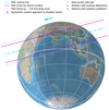 |
Fig. 1 Reconstructed occultation map of the 5 September 2019 event. |
3 Light-curve fitting methods
3.1 Light-curve model
In order to simulate observed light curves, we implemented a light-curve model, ϕ(t; A, s, Δt, Aτ, Δρ, p0), which is described in Appendix C and is consistent with DO15 (Dias-Oliveira et al. 2015; Sicardy et al. 2016, 2021; Meza et al. 2019). As a function of model parameters, its time-dependent Jacobian matrix was also implemented to represent the sensitivity of the model to the corresponding parameters to be estimated through fitting procedures.
The light-curve model of a given station can be formally written as
 (1)
(1)
where i indicates the quantities associated with the station; for further details, the reader is referred to Appendix C. Here, the reference ephemerides we use are the NIMAv95 asteroidal ephemeris (Desmars et al. 2015, 2019) for the orbit of the Pluto system barycenter with respect to the Sun, the PLU0586 satellite ephemerides (Brozovic et al. 2015; Jacobson et al. 2019) for the orbit of Pluto with respect to the Pluto system barycenter, and the DE4408 planetary ephemerides (Park et al. 2021) for the orbits of the Earth and the Sun with respect to the Solar System barycenter. The reference star catalog where the data of the occulted star are obtained is Gaia DR3.
3.2 Fitting procedure
The light-curve model was fitted to the normalized observed light curves simultaneously by nonlinear least squares, returning a χ2-type value of goodness-of-fit. The goal is to minimize the objective function given by
 (2)
(2)
where tij represents the mid-exposure time of the jth observation of the station i.
In addition, with the used reference ephemerides and star catalog, some a priori information on Δρ can be obtained:
 (3)
(3)
where the uncertainty σρ is set to 72 km using the positional uncertainties listed in the “orbit quality” table of NIMAv9 and in Gaia DR3. This σρ value corresponds to about 3 mas on the sky at the geocentric distance of Pluto. The a priori information can be treated as independent observational data and used in the model fitting, with the objective function modified as:
 (4)
(4)
The fitting steps are as follows:
In order to find all local minima at which a nonlinear least-squares fitting could potentially get stuck, we explored the two-parameter space (Δρ, p0) by generating the variation of χ2 as a function of them. Figure 3 presents such two χ2 maps, labeled (a) and (b), which are analyzed in Sect. 4. The maps are generated by minimizing
 or
or  at each fixed (Δρ, p0) point on a regularly spaced grid. The Levenberg-Marquardt (LM) method, which is implemented in the LMFIT package8, was used in each fitting procedure. The free parameters to be adjusted are Δτ9, Δti of any station with no reliable time reference system like QHY1 4GPS, and si and Ai of each station.
For a more accurate best-fitting solution for (Δρ, p0), the LM method is used again, with Δρ and p0 adjusted with initial guesses located at all known local minima of each χ2 map.
Each χ2 map, which provides information about the quality of the fit, is used to define confidence limits based on constant χ2 boundaries (Press et al. 2007).
4 Results
Figure 3a shows the  map for the 5 September 2019 occultation. Two local minima are observed. However, considering the significant χ2 difference of 9 between the two local minima, the global minimum is more likely to be the correct solution. In addition, the Δρ value at the global minimum is more consistent with the NIMAv9 solution, Δρ = 0 km, at the 0.16 σρ level, compared with the other local one at the 2.44 σρ level.
In an effort to mitigate or at least further weaken the presence of multiple local minima, we calculated the  map by adding the χ2-type value of the a priori information, (Δρ/σρ)2, into the
  map. Figure 3b presents the results, which show that two local minima are still present, but with a χ2 difference of about 14.5, which is larger than that of the
  map. Therefore, the global minimum is confidently accepted as the solution for (ρcag, psurf), as provided in Table 1.
Moreover, Fig. 3 presents the consistency of our derived psurf across the two different local minima. Our findings demonstrate that the specific choice of local minima does not significantly affect the value of psurf, further supporting the reliability of our solution for psurf.
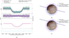 |
Fig. 2 Occultation observations and the best-fitting light-curve model of the 5 September 2019 event. Panel a: observed and simultaneously fitted light curves. Panels b and c: reconstructed stellar paths seen by DWM and HNU, respectively. |
5 Pressure evolution
5.1 Comparisons and necessary reanalyses of historical events
In Fig. 4, the red plot represents our psurf measurement from the 5 September 2019 occultation. We also include other published measurements (Hinson et al. 2017; Meza et al. 2019; Arimatsu et al. 2020; Young et al. 2021; Sicardy et al. 2021) and the pressure evolution predicted by the VTM19 in order to provide a comprehensive view of the pressure variations on Pluto.
To avoid potential inconsistencies arising from different analysis methods, as discussed by Sicardy et al. (2021), we reanalyzed the 15 August 2018 event studied by Young et al. (2021) using the IXON observational data of Silva-Cabrera et al. (2022). The derived pressure measurement presented in Appendix D.1 is  µbar. In addition, we also reanalyze the 17 July 2019 event in Appendix D.2, deriving a pressure of
  µbar, which is similar to that of Arimatsu et al. (2020), of
  µbar. This similarity is expected because the same DO15 method is used. As this same method is used by Meza et al. (2019) and Sicardy et al. (2021), their pressure measurements, along with that of Arimatsu et al. (2020), can be fully compared with our new ones. Both the remeasurements are plotted in black in Fig. 4.
The pressure measurement from the 5 September 2019 event shows alignments with those from the 19 July 2016, 15 August 2018, and 6 June 2020 events within their combined 1σ levels. Our new measurement from the 15 August 2018 event does not show the significant pressure drop previously reported by Young et al. (2021). The previously reported pressure drop between the 19 July 2016 and 17 July 2019 events is still detected at the same level as in Arimatsu et al. (2020).
5.2 Discussion on pressure variations
While the VTM19 remains, on average, applicable and capable of predicting the main atmospheric behavior during the observed years, there are also two probable V-shaped pressure variations observed from 2010 to 2015 and from 2015 to 2020, especially when considering the measurements from the 4 June 2011 and 17 July 2019 events. These V-shaped variations suggest the presence of additional factors that have not been accounted for. Specifically, short-term changes in Pluto’s surface ices and their interaction with the atmosphere are likely contributing to the variation. Moreover, spectral monitoring of the surface composition has revealed some short-term changes in the ices over several Earth years (e.g., Grundy et al. 2014; Lellouch et al. 2022; Holler et al. 2022).
However, the validity of the V-shaped variations is debatable given the stellar faintness of the 4 June 2011 event and the grazing single-chord geometry of the 17 July 2019 event. If the debatable measurement from the 17 July 2019 event were discarded, no significant changes would be observed between 2016 and 2020. This more likely supports the plateau phase since 2015 predicted by the VTM19. In order to better understand the relationship between these factors, further observations using multiple observational techniques (occultation, spectroscopy, and photometry) are required, as well as simulations with a refined VTM.
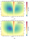 |
Fig. 3 The χ2 maps of the 5 September 2019 event. Panels a and b: The |


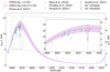 |
Fig. 4 Pressure evolution of Pluto over a 248-yr heliocentric orbital period predicted by the VTM19, along with the measured pressures with 1σ error bars. The 3σ error bars of our new measurements and of the previous measurements of the 19 July 2016, 17 July 2019, and 6 June 2020 events are also presented using the published χ2 maps. |

6 Conclusions
The unique observations of the 5 September 2019 occultation provide a surface pressure of psurf = 11.478 ± 0.55 µbar. In order to avoid potential method inconsistencies in comparing with historical pressure measurements (Sicardy et al. 2021), we also reanalyzed the 15 August 2018 and 17 July 2019 events based on publicly available data (Silva-Cabrera et al. 2022; Arimatsu et al. 2020). All measurements are presented in Fig. 4.
The VTM 19 remains applicable on average. In addition, we also observed unaccounted-for V-shaped pressure variations with the previously reported pressure drop being a part of these variations; however, these variations are debatable. To better understand all significant pressure variations of Pluto, continuous pressure monitoring through occultation observations is essential where possible. Also, simultaneous and frequent spectroscopic and photometric monitoring of changes to its surface ice are important, as such comprehensive monitoring will provide more short-term and long-term evolution constraints of Pluto’s interacting atmosphere and surface.
Acknowledgements
We acknowledge Bruno Sicardy for his useful comments that helped improving this manuscript. This work has been supported by the National Natural Science Foundation of China (Grant Nos. 12203105 and 12103091). We acknowledge the science research grants from the China Manned Space Project with NO.CMS-CSST-2021-A12 and No. CMS-CSST-2021-B10. This research has made use of data from the 40 cm DOB telescope at the Dawei Mountain Observatory of Hunan Astronomical Association and from the 50 cm RC telescope at the Observatory of Hebei Normal University. We ackonwledge the support of Chinese amateur astronomers from Hunan Astronomical Association, Nanjing Amateur Astronomers Association, and Shenzhen Astronomical Observatory Team.
Appendix A Two occultation campaigns in 2019
Stations that encountered weather problems on 17 July 2019
Stations with positive detections on 5 September 2019
Stations that encountered weather problems on 5 September 2019
The 17 July 201910 and the 5 September 201911 stellar occultations by Pluto were originally predicted by the ERC Lucky Star project12.
A.1 The 17 July 2019 occultation campaign
Figure A.1a presents the reconstructed path of the shadow of Pluto13 during the 17 July 2019 event, which was studied by Arimatsu et al. (2020). We also organized an observation campaign involving stations detailed in Table A.1. All the above-mentioned stations are also presented in Figure A.1a. Unfortunately, all our stations encountered weather problems.
A.2 The 5 September 2019 occultation campaign
The occultation map of the 5 September 2019 event is given by Figure 1. Table A.2 lists the circumstances of stations with positive detections. Table A.3 lists the circumstances of stations that encountered weather problems.
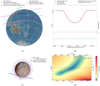 |
Fig. A.1 Reanalysis of the 17 July 2019 event based on the TUHO observational data from Figure 1 of Arimatsu et al. (2020) (credit: Arimatsu et al, A&A, 638, L5, 2020, reproduced with permission © ESO). Panel (a): Reconstructed occultation map. Panel (b): Observed and simultaneously fitted light curves. Panel (c): Reconstructed stellar paths seen by TUHO. Panel (d): The χ2 map, where χ2 denotes the goodness-of-fit value using these data. The best-fitting χ2 value per degree of freedom is 0.860. |
Appendix B Data processing
The observational data were initially obtained in the FITS format, a commonly used format for astronomical data. To process and analyze these data, we used the Tangra occultation photometric tool developed by Pavlov (2020). This tool offers various functionalities and algorithms specifically designed for analyzing occultation events. When calibration images including bias, dark, and flat-field frames are available, they are used for image correction. The default measurement type and tracking method provided by Tangra were applied. The reduction method was aperture photometry with median background subtraction. The combined image of the occulted star and Pluto’s system is circled as the target.
For each station, a selection of suitable guiding and nearby reference stars (typically three) was made. All images of target and reference stars are confirmed as unaffected by overexposure. The signal flux counts, denoted as Isignal, and the background flux counts, denoted as Ibkg, were measured for the target and each reference star in all FITS files. The timing information and measurement results were exported to a CSV file specific to each station, from which the observed light curves would be generated.
Further data processing and analysis were performed using our data reduction code implemented in Python. Each flux measurement for the target or a reference star was calculated as I = Isignal − Ibkg. The measurement error, σI, was modeled using the classical form given by:
 (B.1)
(B.1)
where σbkg is the standard deviation of the background (Ibkg) and geff is the effective gain that represents the number of electrons per flux count.
The relative photometric result of the target is defined as
 (B.2)
(B.2)
where IT is the I of target and IRS the sum of those of all reference stars. This step helps eliminate low-frequency variations caused by atmospheric and instrumental effects. The corresponding measurement error, σF, was derived using the usual formula for propagation of errors (Press et al. 2007).
If the effective gain geff was not precisely known,  was adjusted with the non-negative constraint to fit the derived σF model (
 where
where  ) to the standard deviation of F outside the occultation part.
Finally, the normalized total observed flux, denoted as f, and its error, σ, were derived by dividing F and σF, respectively, by the median of F outside the occultation part. As a result, f outside the occultation part approximates unity.
Appendix C Synthetic light curve model for a stellar occultation by Pluto
For a given station, the light-curve model is represented as:
 (C.1)
(C.1)
where t is the recorded timing of the observation and ϕ is the received flux, as a function of t; A is the total flux of the star and Pluto’s system when the star is not occulted; s is the flux ratio of the occulted star to A; and ψ is the normalized (between zero and unity) flux of the occulted star, which represents the total flux of the primary (sometimes called the near-limb) and secondary (or far-limb, when available) images produced by Pluto’s spherical planetary atmosphere (Sicardy 2023) as shown in Figure 2.
To calculate ψ, the following equation is used:
 (C.2)
(C.2)
where z is the distance of the station to the shadow axis, that is, the line passing through the center of Pluto and parallel to the light ray from the star; r+ and r− represent the closest approach distances of the primary and secondary images to the shadow axis, respectively; and Rp is the radius of Pluto’s body. The dividers, |r±/z|, and derivatives, |dr±/dz|, account for the compression and stretching effects produced by the spherical planetary atmosphere, respectively, caused by limb curvature and differential refraction.
Given reference ephemerides and a star catalog, the distance z is modeled in the International Celestial Reference Frame (ICRF) using the following equation:
 (C.3)
(C.3)
where t + Δti represents the real observation epoch corrected for the camera time recording offset Δti;  is the unit vector in the direction of the geocentric astrometric position of the occulted star; ρi is the geocentric geometric position of i; ρp is the geocentric astrometric position of Pluto obtained at t + Δti + Δτ, with Δτ accounting for the ephemeris offset along the geocentric motion of Pluto;
  is the unit vector in the northern direction along the predicted geocentric closest approach to the shadow axis, multiplied by Δρ to account for the ephemeris offset across the geocentric motion of Pluto. The two ephemeris offset parameters, Δτ and Δρ, represent the corrections to the epoch tcag and distance ρcag of the geoncetric closest approach predicted with the given reference ephemerides and star catalog (see Section 3.1).
Then, the values of r± can be numerically solved using the relationship between z and r±:
 (C.4)
(C.4)
where D represents the light travel distance, which can be approximated by the geocentric distance of Pluto, and ω(r) is the total deviation angle at r.
As detailed in Dias-Oliveira et al. (2015) and Sicardy (2023), ω(r) can be obtained by a ray-tracing code that follows these steps:
set the temperature profile T(r) of Pluto using Equation (4) from Dias-Oliveira et al. (2015), with parameters obtained from Sicardy et al. (2016);
set the gas molecular refractivity K corresponding to a stellar wavelength of λµm;
set the atmospheric pressure p0 at the reference radius r0 of 1215 km either directly, or determined from a surface pressure psurf (at Rp = 1187 km) with the ratio psurf/p0 = 1.837 used by previous studies (Meza et al. 2019; Sicardy et al. 2021);
set the needed boundary condition for the gas molecular density, n0 = p0/(kB · T(r0)), where kB is Boltzmann’s constant;
integrate the first-order differential equation (Equations (5) and (6) of Dias-Oliveira et al. (2015)) to obtain the gas molecular density profile n(r);
transform n(r) to the gas refractivity v(r) using v(r) = K · n(r) (Equation (7) from Dias-Oliveira et al. (2015));
calculate the total deviation based on the straight line approximation (Equation (16) of Sicardy (2023), with the upper limit of r set as 2600 km).
Finally, an interpolator of ω(r) for specific p0 and K values is built in advance. This allows efficient computation of ω(r) during the analysis of the occultation observations.
Appendix D Results of the reanalyzed events necessary for comparisons
D.1 The 15 August 2018 event
Based on the IXON observational data from the online supplemental data file14 of Silva-Cabrera et al. (2022), we reanalyzed the 15 August 2018 event15 using our fitting procedure. As the raw data were normalized, with the flux contribution of the Pluto system carefully removed by Silva-Cabrera et al. (2022), all Ai and si were fixed as unity in our fitting procedure. Moreover, as the uncertainties used for weighting are not given, we used the standard deviation of the data outside the occultation part for each station. Results are presented in Figure D.1. Our surface pressure remeasurement is  µbar.
µbar.
D.2 The 17 July 2019 event
Based on the TUHO observational data and uncertainties from Figure 1 of Arimatsu et al. (2020) (credit: Arimatsu et al, A&A, 638, L5, 2020, reproduced with permission © ESO), we reanalyzed the 17 July 2019 event using our fitting procedure. Results are presented in Figure A.1. Our surface pressure remeasurement is  µbar, similar to the result obtained by Arimatsu et al. (2020),
  µbar.
µbar.
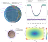 |
Fig. D.1 Reanalysis of the 15 August 2018 event based on the IXON observational data from the online supplemental data file of Silva-Cabrera et al. (2022). The raw data were normalized, with the flux contribution of the Pluto system carefully removed by Silva-Cabrera et al. (2022). The uncertainties used for weighting are the standard deviation of the data outside the occultation part for each station. Panel (a): Reconstructed occultation map. Panel (b): Observed and simultaneously fitted light curves. Panel (c): Reconstructed stellar paths seen by IXON. Panel (d): The χ2 map, where χ2 denotes the goodness-of-fit value using these data. The best-fitting χ2 value per degree of freedom is 1.046. |
References
- Arimatsu, K., Hashimoto, G. L., Kagitani, M., et al. 2020, A&A, 638, A5 [NASA ADS] [CrossRef] [EDP Sciences] [Google Scholar]
- Bertrand, T., & Forget, F. 2016, Nature, 540, 86 [NASA ADS] [CrossRef] [Google Scholar]
- Bertrand, T., Forget, F., Umurhan, O. M., et al. 2018, Icarus, 309, 277 [NASA ADS] [CrossRef] [Google Scholar]
- Bertrand, T., Forget, F., Umurhan, O. M., et al. 2019, Icarus, 329, 148 [NASA ADS] [CrossRef] [Google Scholar]
- Bosh, A. S., Person, M. J., Levine, S. E., et al. 2015, Icarus, 246, 237 [NASA ADS] [CrossRef] [Google Scholar]
- Brosch, N. 1995, MNRAS, 276, 571 [NASA ADS] [Google Scholar]
- Brozovic, M., Showalter, M. R., Jacobson, R. A., & Buie, M. W. 2015, Icarus, 246, 317 [CrossRef] [Google Scholar]
- Buie, M. W., Leiva, R., Keller, J. M., et al. 2020a, AJ, 159, 230 [CrossRef] [Google Scholar]
- Buie, M. W., Porter, S. B., Tamblyn, P., et al. 2020b, AJ, 159, 130 [NASA ADS] [CrossRef] [Google Scholar]
- Desmars, J., Camargo, J. I. B., Braga-Ribas, F., et al. 2015, A&A, 584, A96 [NASA ADS] [CrossRef] [EDP Sciences] [Google Scholar]
- Desmars, J., Meza, E., Sicardy, B., et al. 2019, A&A 625, A43 [NASA ADS] [CrossRef] [EDP Sciences] [Google Scholar]
- Dias-Oliveira, A., Sicardy, B., Lellouch, E., et al. 2015, ApJ, 811, 53 [NASA ADS] [CrossRef] [Google Scholar]
- Elliot, J. L., Dunham, E. W., Bosh, A. S., et al. 1989, Icarus, 77, 148 [NASA ADS] [CrossRef] [Google Scholar]
- Elliot, J. L., Ates, A., Babcock, B. A., et al. 2003, Nature, 424, 165 [NASA ADS] [CrossRef] [Google Scholar]
- Forget, F., Bertrand, T., Vangvichith, M., et al. 2017, Icarus, 287, 54 [NASA ADS] [CrossRef] [Google Scholar]
- Gaia Collaboration 2022, VizieR Online Data Catalog: I/355 [Google Scholar]
- Gaia Collaboration (Vallenari, A., et al.) 2023, A&A, 674, A1 [NASA ADS] [CrossRef] [EDP Sciences] [Google Scholar]
- Grundy, W. M., Olkin, C. B., Young, L. A., & Holler, B. J. 2014, Icarus, 235, 220 [NASA ADS] [CrossRef] [Google Scholar]
- Gulbis, A. A. S., Emery, J. P., Person, M. J., et al. 2015, Icarus, 246, 226 [CrossRef] [Google Scholar]
- Hinson, D. P., Linscott, I. R., Young, L. A., et al. 2017, Icarus, 290, 96 [CrossRef] [Google Scholar]
- Holler, B. J., Yanez, M. D., Protopapa, S., et al. 2022, Icarus, 373, 114729 [NASA ADS] [CrossRef] [Google Scholar]
- Hubbard, W. B., Hunten, D. M., Dieters, S. W., Hill, K. M., & Watson, R. D. 1988, Nature, 336, 452 [NASA ADS] [CrossRef] [Google Scholar]
- Jacobson, R. A., Brozovic, M., Showalter, M., et al. 2019, in Pluto System After New Horizons, 2133, 7031 [NASA ADS] [Google Scholar]
- Lellouch, E., Butler, B., Moreno, R., et al. 2022, Icarus, 372, 114722 [NASA ADS] [CrossRef] [Google Scholar]
- Meza, E., Sicardy, B., Assafin, M., et al. 2019, A&A 625, A42 [NASA ADS] [CrossRef] [EDP Sciences] [Google Scholar]
- Morgado, B. E., Sicardy, B., Braga-Ribas, F., et al. 2021, A&A, 652, A141 [NASA ADS] [CrossRef] [EDP Sciences] [Google Scholar]
- Morgado, B. E., Gomes-Júnior, A. R., Braga-Ribas, F., et al. 2022, AJ, 163, 240 [NASA ADS] [CrossRef] [Google Scholar]
- Newell, D., & Tiesinga, E. 2019, in The International System of Units (SI) Special Publication (NIST SP), National Institute of Standards and Technology, Gaithersburg, MD, https://doi.org/10.6028/NIST.SP.330-2019 [CrossRef] [Google Scholar]
- Olkin, C. B., Young, L. A., Borncamp, D., et al. 2015, Icarus, 246, 220 [NASA ADS] [CrossRef] [Google Scholar]
- Park, R. S., Folkner, W. M., Williams, J. G., & Boggs, D. H. 2021, AJ, 161, 105 [NASA ADS] [CrossRef] [Google Scholar]
- Pasachoff, J. M., Souza, S. P., Babcock, B. A., et al. 2005, AJ, 129, 1718 [CrossRef] [Google Scholar]
- Pasachoff, J. M., Babcock, B. A., Durst, R. F., et al. 2017, Icarus, 296, 305 [CrossRef] [Google Scholar]
- Pavlov, H. 2020, Astrophysics Source Code Library [record ascl:2004.002] [Google Scholar]
- Pereira, C. L., Sicardy, B., Morgado, B. E., et al. 2023, A&A, 673, A4 [Google Scholar]
- Person, M. J., Dunham, E. W., Bosh, A. S., et al. 2013, AJ, 146, 83 [NASA ADS] [CrossRef] [Google Scholar]
- Person, M. J., Bosh, A. S., Zuluaga, C. A., et al. 2021, Icarus, 356, 113572 [NASA ADS] [CrossRef] [Google Scholar]
- Press, W. H., Teukolsky, S. A., Vetterling, W. T., & Flannery, B. P. 2007, Numerical Recipes in C++: The Art of Scientific Computing, 3rd edn. (Cambridge University Press) [Google Scholar]
- Rannou, P., & Durry, G. 2009, J. Geophys. Res. Planets, 114, E11013 [NASA ADS] [CrossRef] [Google Scholar]
- Sicardy, B. 2023, Comptes Rendus Physique, 23, 213 [NASA ADS] [CrossRef] [Google Scholar]
- Sicardy, B., Widemann, T., Lellouch, E., et al. 2003, Nature, 424, 168 [NASA ADS] [CrossRef] [Google Scholar]
- Sicardy, B., Bolt, G., Broughton, J., et al. 2011, AJ, 141, 67 [CrossRef] [Google Scholar]
- Sicardy, B., Talbot, J., Meza, E., et al. 2016, ApJ, 819, L38 [NASA ADS] [CrossRef] [Google Scholar]
- Sicardy, B., Ashok, N. M., Tej, A., et al. 2021, ApJ, 923, L31 [NASA ADS] [CrossRef] [Google Scholar]
- Silva-Cabrera, J. S., Castro-Chacón, J. H., Reyes-Ruiz, M., et al. 2022, MNRAS, 511, 5550 [NASA ADS] [CrossRef] [Google Scholar]
- Stern, S. A., Bagenal, F., Ennico, K., et al. 2015, Science, 350, aad1815 [Google Scholar]
- Washburn, E. W., West, C. J., Dorsey, N. E., et al. 1930, International Critical Tables of Numerical Data, Physics, Chemistry and Technology (Washington, DC: The National Academies Press) [Google Scholar]
- Yelle, R. V., & Elliot, J. L. 1997, in Pluto and Charon, eds. S. A. Stern, & D. J. Tholen (Kluwer Academic Publishers), 347 [Google Scholar]
- Young, E. F., French, R. G., Young, L. A., et al. 2008, AJ, 136, 1757 [NASA ADS] [CrossRef] [Google Scholar]
- Young, E., Young, L. A., Johnson, P. E., & PHOT Team 2021, AAS Meet. Abstr., 53, 307.06 [NASA ADS] [Google Scholar]
Sputnik Planitia is a large plain or basin on Pluto discovered by the New Horizons spacecraft (Stern et al. 2015).
The occulted star is Gaia DR3 6771712487062767488, of which the astrometric and photometric parameters are obtained from VizieR (Gaia Collaboration 2022).
As a technical note, if no equipment for reliable time references is used, Δτ should be fixed as zero, avoiding fitting problems caused by its linear relationship with ti.
The occulted star is Gaia DR3 6772059623498733952, of which the astrometric and photometric parameters are obtained from VizieR.
“stac401_Supplement_File - zip file”, via the paper link https://doi.org/10.1093/mnras/stac401.
The occulted star is Gaia DR3 6772629170525258240, of which the astrometric and photometric parameters are obtained from VizieR.
All Tables
All Figures
|
Fig. 1 Reconstructed occultation map of the 5 September 2019 event. |
| In the text | |
|
Fig. 2 Occultation observations and the best-fitting light-curve model of the 5 September 2019 event. Panel a: observed and simultaneously fitted light curves. Panels b and c: reconstructed stellar paths seen by DWM and HNU, respectively. |
| In the text | |
|
Fig. 3 The χ2 maps of the 5 September 2019 event. Panels a and b: The |
| In the text | |
|
Fig. 4 Pressure evolution of Pluto over a 248-yr heliocentric orbital period predicted by the VTM19, along with the measured pressures with 1σ error bars. The 3σ error bars of our new measurements and of the previous measurements of the 19 July 2016, 17 July 2019, and 6 June 2020 events are also presented using the published χ2 maps. |
| In the text | |
|
Fig. A.1 Reanalysis of the 17 July 2019 event based on the TUHO observational data from Figure 1 of Arimatsu et al. (2020) (credit: Arimatsu et al, A&A, 638, L5, 2020, reproduced with permission © ESO). Panel (a): Reconstructed occultation map. Panel (b): Observed and simultaneously fitted light curves. Panel (c): Reconstructed stellar paths seen by TUHO. Panel (d): The χ2 map, where χ2 denotes the goodness-of-fit value using these data. The best-fitting χ2 value per degree of freedom is 0.860. |
| In the text | |
|
Fig. D.1 Reanalysis of the 15 August 2018 event based on the IXON observational data from the online supplemental data file of Silva-Cabrera et al. (2022). The raw data were normalized, with the flux contribution of the Pluto system carefully removed by Silva-Cabrera et al. (2022). The uncertainties used for weighting are the standard deviation of the data outside the occultation part for each station. Panel (a): Reconstructed occultation map. Panel (b): Observed and simultaneously fitted light curves. Panel (c): Reconstructed stellar paths seen by IXON. Panel (d): The χ2 map, where χ2 denotes the goodness-of-fit value using these data. The best-fitting χ2 value per degree of freedom is 1.046. |
| In the text | |
Current usage metrics show cumulative count of Article Views (full-text article views including HTML views, PDF and ePub downloads, according to the available data) and Abstracts Views on Vision4Press platform.
Data correspond to usage on the plateform after 2015. The current usage metrics is available 48-96 hours after online publication and is updated daily on week days.
Initial download of the metrics may take a while.