| Issue |
A&A
Volume 679, November 2023
|
|
|---|---|---|
| Article Number | A56 | |
| Number of page(s) | 22 | |
| Section | Planets and planetary systems | |
| DOI | https://doi.org/10.1051/0004-6361/202346022 | |
| Published online | 03 November 2023 | |
Shape models and spin states of Jupiter Trojans
Testing the streaming instability formation scenario★
1
Charles University, Faculty of Mathematics and Physics, Institute of Astronomy,
V Holešovičkách 2,
18000
Prague 8, Czech Republic
e-mail: This email address is being protected from spambots. You need JavaScript enabled to view it.
2
Department of Space Studies, Southwest Research Institute,
1050 Walnut St., Suite 300,
Boulder, CO
80302, USA
3
Center for Solar System Studies,
9302 Pittsburgh Ave. Suite 200,
Rancho Cucamonga, CA
91730, USA
4
Belgrade Astronomical Observatory,
Volgina 7,
11060
Belgrade 38, Serbia
5
Blue Mountains Observatory,
Leura, Australia
6
Department of Physics, The Catholic University of America,
Washington, DC
20064, USA
7
Astrophysics Science Division, NASA Goddard Space Flight Center,
Greenbelt, MD
20771, USA
8
Center for Research and Exploration in Space Science and Technology, NASA/GSFC,
Greenbelt, MD
20771, USA
Received:
30
January
2023
Accepted:
26
June
2023
Abstract
The leading theory for the origin of Jupiter Trojans (JTs) assumes that JTs were captured to their orbits near the Lagrangian points of Jupiter during the early reconfiguration of the giant planets. The natural source region for the majority of JTs would then be the population of planetesimals born in a massive trans-Neptunian disk. If true, JTs represent the most accessible stable population of small Solar System bodies that formed in the outer regions of the Solar System. For this work, we compiled photometric datasets for about 1000 JTs and applied the convex inversion technique in order to assess their shapes and spin states. We obtained full solutions for 79 JTs, and partial solutions for an additional 31 JTs. We found that the observed distribution of the pole obliquities of JTs is broadly consistent with expectations from the streaming instability, which is the leading mechanism for the formation of planetesimals in the trans-Neptunian disk. The observed JTs’ pole distribution has a slightly smaller prograde vs. retrograde asymmetry (excess of obliquities >130°) than what is expected from the existing streaming instability simulations. However, this discrepancy can be plausibly reconciled by the effects of the post-formation collisional activity. Our numerical simulations of the post-capture spin evolution indicate that the JTs’ pole distribution is not significantly affected by dynamical processes such as the eccentricity excitation in resonances, close encounters with planets, or the effects of nongravitational forces. However, a few JTs exhibit large latitude variations of the rotation pole and may even temporarily transition between prograde- and retrograde-rotating categories.
Key words: minor planets, asteroids: individual: Jupiter Trojans / surveys / methods: numerical / methods: data analysis
Tables B.1–B.5 are available at the CDS via anonymous ftp to cdsarc.cds.unistra.fr (130.79.128.5) or via https://cdsarc.cds.unistra.fr/viz-bin/cat/J/A+A/679/A56
© The Authors 2023
 Open Access article, published by EDP Sciences, under the terms of the Creative Commons Attribution License (https://creativecommons.org/licenses/by/4.0), which permits unrestricted use, distribution, and reproduction in any medium, provided the original work is properly cited.
This article is published in open access under the Subscribe to Open model. This email address is being protected from spambots. You need JavaScript enabled to view it. to support open access publication.
1 Introduction
Jupiter Trojans (JTs) are minor bodies co-orbiting with Jupiter in the proximity of its Lagrangian points L4 and L5. Bodies librating about the leading L4 point are commonly referred to as the Greek camp (or clan or group), while those near the trailing L5 point are referred to as the Trojan camp. As for the currently known population of Greeks and Trojans, we adopt in this work a list of JTs as identified by the orbit classification flags in the MPC Orbit (MPCORB) database1.
The origin of JTs remains an open problem. The currently leading theory assumes that JTs were captured to their orbits near the Lagrangian points during the early reconfiguration of the giant planets (Morbidelli et al. 2005; Nesvorný et al. 2013). The natural source region for the majority of JTs would then be the population of planetesimals born in a massive trans-Neptunian disk. As a result, JTs should share the physical properties of the currently observed trans-Neptunian objects (TNOs), as well as the comets and irregular satellites of giant planets. Other theories avoid involving the planetary reconfiguration event and postulate that JTs formed at their current location together with Jupiter (see reviews in Marzari et al. 2002; Emery et al. 2015), or were born in the Jupiter co-orbital zone and accompanied its early inward migration (Pirani et al. 2019). In this paper, we adopt the capture model for JTs as a baseline hypothesis, because several other pieces of evidence support the view that giant planets underwent a violent instability at some early moment of the Solar System evolution (see, e.g., Nesvorný 2018). In any case, studying the physical properties of JTs is an obvious way how to test various theories of the JTs’ origin and eventually decide which theory is more in line with the observing evidence. In fact, this is also one of the main goals of our work.
Previous physical studies have already revealed interesting properties of JTs. For instance, analysis of visible and near-infrared spectra suggested that a color bimodality exists in the JTs’ population (e.g., Emery et al. 2011; Wong & Brown 2016): the majority of bodies belong to the so-called red (D-type) and less red (P-type) groups. This color bimodality hints at the relationship between the spectral properties of JTs and of comets and TNOs. On the other hand, C-type bodies, which represent about 10% of the JT population and – for instance – include the largest collisional JT family Eurybates, are spectrally more similar to a primitive outer asteroidal belt or Cybele group objects (Fornasier et al. 2007; De Luise et al. 2010).
In closer relation to our work, we note that a significant amount of data was collected about JTs’ rotation rate since the 1980s (see reviews in Barucci et al. 2002; Emery et al. 2015). Hints from these early studies have been recently confirmed and extended by analysis of space-born observations from Kepler and Transiting Exoplanet Survey Satellite (TESS), and dedicated survey programs using large ground-based instruments (e.g., Szabó et al. 2016; Ryan et al. 2017; Kalup et al. 2021; Chang et al. 2021). These studies find (i) an excess (possibly even separate population) of slowly rotating objects, and (ii) a presence of a size-dependent lower limit of the rotation period, such that smaller JTs may reach shorter periods to near 4 h, while larger JTs tend to have this limit near 5 h. The latter nicely supports a rubble-pile structure of JTs with a characteristic bulk density of ≃0.9 g cm−3, and the emerging role of the Yarkovsky-O’Keefe-Radzievski-Paddack (YORP) effect for small JTs (e.g., Vokrouhlický et al. 2015). The population of unusually slowly rotating JTs is interesting in the context of our work since it has been linked to unbound components from tidally evolved binary planetesimals captured among Trojans (Nesvorný et al. 2020).
While a significant amount of data about the rotation rates of JTs have been collected and analyzed, much less is presently known about the complete characterization of their spin state (i.e., rotation rate and pole direction). Here we aim to fill this missing piece of information by deriving rotation state properties and convex shapes for many JTs. Particularly, we are interested in the direction of the rotation axis with respect to the orbital plane – the pole obliquity. This parameter reflects the object’s dynamical history and could help constrain various theories aiming to explain the population’s origin.
Our paper is organized as follows. We gathered available optical photometric data (Sect. 2) from various sources and analyzed them using a convex inversion method (Kaasalainen et al. 2001; Kaasalainen & Torppa 2001) following, with some minor adjustments, the scheme of Hanuš et al. (2021; Sect. 3). We present derived physical properties in Sect. 4. Adopting the capture model for JTs, we also performed numerical simulations to (i) access the original spin distribution of the planetesimal population that is assumed to be the source population of JTs (Sect. 5), and (ii) estimate the post-capture spin evolution of JTs (Sect. 6). Finally, we discuss our findings in Sect. 7, and conclude our work in Sect. 8.
2 Data
We gathered optical disk-integrated photometry from various sources. First, data for asteroids with published shape models are usually available in the Database of Asteroid Models from Inversion Techniques2 (DAMIT; Ďurech et al. 2010). Additional dense-in-time light curves were downloaded from the ALCDEF3 database or were obtained from individual observers. Moreover, we also make use of sparse-in-time photometric data from various surveys. These include Catalina Sky Survey (CSS; Larson et al. 2003), the US Naval Observatory in Flagstaff (USNO-Flagstaff), the Asteroid Terrestrial-impact Last Alert System (ATLAS; Tonry et al. 2018), the All-Sky Automated Survey for Supernovae (ASAS-SN; Shappee et al. 2014; Kochanek et al. 2017; Hanuš et al. 2021), Gaia Data Release 3 (Gaia DR3; Tanga et al. 2023; Babusiaux et al. 2023), the Zwicky Transient Facility (ZTF; Bellm et al. 2019), Kepler K2 (Szabó et al. 2016; Kalup et al. 2021), Palomar Transient Factory (PTF; Waszczak et al. 2015), and TESS (Pál et al. 2020).
Individual photometric measurements from CSS, USNO-Flagstaff, and ZTF are available via AstDyS-2 database4, from where we downloaded them and processed them following the approach of Hanuš et al. (2011). Data from ASAS-SN, Gaia DR3, K2, TESS, and PTF were released together with the corresponding publications. We downloaded the data from the repositories and processed them similarly to the other sparsein-time data. We already used ATLAS and ASAS-SN data in previous studies (Ďurech et al. 2020; Hanuš et al. 2021), to which we refer for additional information about the data processing.
Altogether, we obtained optical datasets for 1009 JTs. In all cases, sparse-in-time datasets are included, usually from multiple sources. Dense-in-time light curves are available for a subsample of 164 JTs.
3 Light curve inversion
We analyzed the optical photometry data using the convex inversion method (Kaasalainen et al. 2001; Kaasalainen & Torppa 2001). This commonly used gradient-based inversion method represents the shape model as a convex polyhedron; convexity is a necessary assumption for the shape solution to be stable and unique as only disk-integrated data are utilized (Kaasalainen & Lamberg 2006). The method converges to a unique shape solution for fixed values of the rotation state parameters – sidereal rotation period and spin axis orientation5. Including these (usually unknown) parameters into the optimization, the χ2 behavior over the parameter space becomes complicated by having a myriad of local minima. The most common, albeit computationally cumbersome, way how to find the global minimum in the parameter space is to analyze all the relevant local minima. In practice, this represents undergoing a CPU time-consuming procedure of running convex inversion for all relevant combinations of rotation state parameters and constructing the corresponding χ2 maps.
We followed the shape modeling procedure described in Hanuš et al. (2021) with one major difference – data weighting. By definition, the best model is defined as having the lowest χ2 value. In order to compute χ2, one should know the uncertainty of individual observations, especially when multisource datasets are utilized. However, these uncertainties are generally not known or are not reliable for the majority of data we have. Moreover, the data we utilized have very different uncertainty – from precise Gaia photometry and high-quality dense light curves, to usually noisy sparse data from sky surveys.
To assign realistic weights to individual datasets, we estimated their characteristic uncertainty by computing RMS residuals for existing shape models in the DAMIT database. Our procedure was as follows. First, we selected data for asteroids with models in DAMIT for each sparse dataset. We used the period and pole parameters as initial values for the optimization and applied the light curve inversion method. For each model, we computed the final RMS and assumed that this number is a proxy for the uncertainty of the measurements. In Fig. 1, we plot RMS values as a function of mean apparent brightness for all datasets. There is a general trend of increasing RMS with increasing magnitude, which naturally arises from the fact that fainter asteroids have larger photometric uncertainties. An exception is Catalina Sky Survey, for which brighter asteroids have also larger errors, likely due to saturation. For each dataset, we fit a quadratic function for the RMS vs. magnitude m dependence with constant parts outside the central interval:
 (1)
(1)
where A, B, and C are free parameters and m is the brightness in magnitudes. This function (red curve in Fig. 1) was then used to compute formal errors of all datasets for all asteroids. The magnitude was computed as a mean apparent brightness over all data.
Although this approach has several caveats – DAMIT models are not fully realistic, the brightness changes significantly for one asteroid due to observing geometry, telescope photometric performance can change during its operation, etc. – it serves well for our purpose to assign operationally acceptable relative weights to different datasets.
The relative weights wi of all available datasets for each asteroid were then computed by
 (2)
(2)
where RMSi is the formal error for each dataset.
Finally, we normalized wi such that
 (3)
(3)
where N is the number of light curves in the dataset. Each sparse dataset is considered as a single light curve.
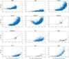 |
Fig. 1 RMS values as a function of mean brightness for all available sparse datasets. The red curve represents a fit to the data defined by the quadratic approximation (and constant parts) in Eq. (1). |
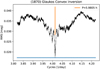 |
Fig. 2 Periodogram in the rotation frequency domain for L5 JT (1870) Glaukos. The black line connects the minima over the trial runs sampling all local RMS values at a fixed rotation period but walking through all other parameters of the model. The blue horizontal line indicates the RMS threshold as defined by Eq. (4), while the orange vertical line represents the best-fitting sidereal rotation period. |
4 Spin and shape modeling of JTs
In total, we applied the convex inversion to 881 JTs with a sufficient amount of photometric measurements. Following the standard modeling approach (e.g., Hanuš et al. 2021), we constructed the periodogram for each asteroid (see an example in Fig. 2). To reduce the CPU time requirements, whenever available, we searched the period only on a short interval near the reported period in the LightCurve DataBase (LCDB, Warner et al. 2009). We considered the reliability of the reported values (through the validity flag) by selecting larger period intervals for less reliable periods. For poor period estimates or unknown periods, we searched for the period on an interval of 2–5000 h.
We considered the period as unique if the best-fitting (i.e., global) solution with  is the only one within the threshold of
 (4)
(4)
where v is the number of degrees of freedom (number of observations minus the number of free parameters). We consider three parameters for the description of the rotation state, three parameters for the scattering law, and 72 parameters for the shape model (55 free parameters in total).
Next, we searched the pole orientation by scanning tens of different values isotropically distributed on a sphere. We then set the same condition for the unique solution as for the period search (Eq. (4)). Due to the symmetry of the light curve inversion problem (Kaasalainen & Lamberg 2006), two pole solutions usually have similar fits – they have a similar shape model and the pole-latitude, but their pole-longitude is ≃180° different.
4.1 Partial solutions and new rotation period estimates
For 31 JTs, we obtained more than two pole solutions within the χ2 threshold set by Eq. (4). Although we are not able to report the unique spin state and shape solution in these cases, the rotation period is derived unambiguously. Moreover, for the majority of these so-called partial solutions, the pole-ecliptic latitude is well constrained (i.e., is similar within the multiple pole solutions), and therefore, it is possible to decide whether the asteroid is a prograde or a retrograde rotator (see Table B.1). Interestingly, Table B.1 contains 11 JTs with no prior value of the rotation period in the LCDB database (e.g., 6997, 15 398, 32370). In the remaining 20 cases, our sidereal rotation periods are consistent with the LCDB rotation periods. Our values usually have smaller uncertainty than the synodic periods from the LCDB, often reaching fractions of a second.
4.2 New and improved shape and rotation state solutions
For 79 JTs, we derived their unique spin state and shape solutions (Table B.2). We visually checked the periodograms and the fit to the light curve data and rejected all suspicious solutions. We also computed the principal moments of inertia (Dobrovolskis 1996) for each shape model solution and dismissed those that were non-physical. Finally, we also compared derived rotation periods with those from the LCDB database and individually investigated all inconsistent cases. We identified six such cases, but none of them is significant, because their LCDB reliability flags indicate that the synodic rotation period estimates could be inaccurate, and thus still consistent with our new, not too different, values.
As there is an overlap between our solutions and their availability in DAMIT, we also verified their consistency. However, these models are usually not fully independent as some of the optical data are mutual. Despite that, the DAMIT solutions represent a useful reliability check of the methodology. The overlap with the DAMIT database is for 13 JTs. Additionally, we considered the spin state solution for (884) Priamus of Stephens (2017) here, although it has not yet been included in DAMIT. We list all the previous spin state solutions in Table B.2.
Six solutions differ by more than 30 degrees in the pole direction, while all the rotation periods are very similar. The inconsistent solutions are for (659) Nestor, (911) Agamemnon, (3391) Sinon, (4489) Dracius, (4709) Ennomos, and (15663) Periphas. The previous solutions, all published in Ďurech et al. (2019), are based on combined Gaia DR2 and Lowell data. As especially the Lowell data have poor photometric accuracy, it is not surprising that the revised models could be significantly different considering the spin vector direction. Interestingly, the solutions usually agree in ecliptic pole-latitude but differ in pole-longitude. Our solutions are based on substantially larger photometric datasets including, in some cases, dense light curves, therefore we prefer those. Moreover, in some cases, we either rejected one of the two previously reported pole solutions or have the mirror solution (i.e., two poles) instead of a single pole. The remaining 65 shape model solutions are new – we list the physical properties of these JTs in Table B.2.
We provide optical data of asteroids with new and revised shape model solutions that are not included in DAMIT in Table B.5. New and revised solutions will be available in the DAMIT database (optical light curves, light curve fits, rotation state parameters, and shape models).
4.3 Assessing the model uncertainties by bootstrapping the photometric datasets
In order to assess the pole and shape uncertainties quantitatively, we performed additional modeling. For asteroids with shape and spin state solutions from Sect. 4.2, we bootstrapped their photometric datasets and applied the convex inversion. We created the bootstrapped datasets for each asteroid by the following procedure: We randomly selected N dense light curves from the original dense dataset of N light curves. Therefore, the bootstrapped datasets could contain individual light curves multiple times, while some have to be inevitably omitted. The sparse datasets were bootstrapped internally: We randomly selected the same number of measurements as in the original sparse dataset from each sparse data source (i.e., ASAS-SN, ATLAS, etc.). We computed the weights following the procedure described in Sect. 3.
In the shape modeling, we used the nominal spin state solutions as initial inputs and found the bootstrapped solutions near these local minima. We repeated the modeling with ten different bootstrapped datasets. We summarize the mean values and standard deviations of pole directions within the bootstrapped solutions in Table B.4. This gives us a rough estimate of the uncertainty – usually below 5 degrees, and quite rarely >10 degrees. Moreover, we also constructed the cumulative obliquity distributions for each bootstrapped dataset to assess its stability later in Sect. 4.5.
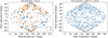 |
Fig. 3 Spin vector distribution of JTs (left panel) and of main belt asteroids with sizes >50 km for comparison (right panel). Spin vectors of MBAs are taken from the DAMIT database. If two possible pole solutions exist, typically separated by ≃180° in longitude, we plot both. L4 and L5 represent the two camps of JTs. |
4.4 Stellar occultations
For eight JTs listed in Tables B.2 and B.3, there were successfully observed stellar occultations with a sufficient number of chords that enabled us to scale the shape models and in some cases also to reject one of the two possible pole solutions. The stellar occultations were assessed through the Occult soft-ware6. A thorough description of the occultation data can be found in Herald et al. (2020). For comparing the occultations with our shape models, we used the same approach as Ďurech et al. (2011). We computed the orientation of the shape model at the time of the occultation, projected it to the fundamental plane, and fit the asteroid’s size to get the best agreement between the model’s silhouette and observed chords. This way, we scaled models of (588) Achilles (Fig. A.2), (884) Pria-mus (Fig. A.3), (911) Agamemnon (Fig. A.4), (1437) Diomedes (Fig. A.5), (1867) Deiphobus (Fig. A.6), (2207) Antenor (Fig. A.7), (4709) Ennomos (Fig. A.8), and (31344) Agathon (Fig. A.9). If one of the two possible pole solutions gave a significantly better agreement with the occultation, we rejected the second pole – this concerns JTs Priamus, Diomedes, and Agathon. We indicate these cases in Table B.2.
For Deiphobus the agreement between the occultation and the shape projection was suboptimal. Therefore, we also reconstructed the shape model by a different approach – by the All-Data Asteroid Modelling (ADAM) inversion technique (Viikinkoski et al. 2015; Viikinkoski 2016). ADAM allows using the stellar occultation for the shape reconstruction contrary to the convex inversion where the shape is scaled in size only. The ADAM shape model of Deiphobus agrees better with the occultation and provides a more realistic size estimate. The alternative ADAM model is listed in Table B.2.
4.5 Spin states of JTs
Our analysis is based on full shape and spin state solutions of 90 JTs – 79 from Sect. 4.2 and 11 solutions adopted from DAMIT (Table B.3), and partial models of 31 JTs (Sect. 4.1). We identified 49 members of the L4 cloud and 72 of the L5 cloud. In what follows, we focus on the analysis of the rotation pole distribution, as this is a new result in this paper. We omit to comment on the rotation rate distribution. This is because previous works, such as Szabó et al. (2016), Ryan et al. (2017), Kalup et al. (2021), Chang et al. (2021) covered this issue with even more data.
In the left panel of Fig. 3, we show the pole directions for JTs. The pole distribution is consistent with being grossly isotropic, similar to the pole distribution among the large (D > 50 km) main-belt asteroids (for models in DAMIT) that is shown in the right panel of Fig. 3 for comparison. Both populations consist of bodies that are large enough not to be significantly affected by the YORP effect, so the pole directions should primarily reflect the initial distribution in the source region and possibly modification due to the collision history (if important enough). The nonuniform distribution of poles caused by the YORP effect is evident only for main-belt asteroids with D < 30 km (Hanuš et al. 2011). Unfortunately, we do not have spin state solutions for such small (D < 30 km) JTs. So far, the first tentative evidence of the YORP effect acting on JTs < 10–20 km was reported by Chang et al. (2021) – smaller JTs have a lower limit of the rotation period near 4 h than the previously published result of 5 h found for larger JTs. There is no obvious difference between the pole orientations within the L4 and L5 clouds.
Deciding the sense of rotation with respect to the orbital plane requires the knowledge of the spin obliquity ε. We computed the obliquity for cases with the full spin solutions. We consider the sense of rotation to be inconclusive if the obliquity is between 80° and 100°, while obliquity <80° indicates a prograde rotator and obliquity >100° a retrograde rotator in our simple approach. We find there are more prograde rotators than retrograde ones in our sample, namely 49 versus 33. This hints at a factor of ≃1.5 between a number of prograde and retrograde populations, or ≃60% abundance of prograde rotators in the overall JT population. We shall operationally work with this result while admitting that the hypothesis of a similar number of prograde and retrograde rotators among JTs may be valid at ≃10% level due to the small size of the sample. For instance, if the sample is doubled, and the ratio of the prograde vs retrograde solutions remains ≃1.5, the room for the isotropy would shrink to only about 1.5% probability. This is a large motivation for determining more spin models among JTs. By splitting the sample at obliquity equal to 90°, we have 54 prograde vs. 36 retrograde JTs, thus a similar abundance of prograde rotators. Due to a larger sample, the significance of the isotropy of the spin poles of JTs decreases to the ≃7% level. The excess in prograde rotators is also present considering the two clouds: there are 22 prograde and 18 retrograde rotators within the L4 cloud (55% vs. 45%), and 32 prograde and 17 retrograde rotators within the L5 cloud (65% vs. 35%).
In Fig. 4, we show the cumulative obliquity distribution of JTs, which provides more complete information than just the simple ratio between the number of prograde and retrograde rotators. Additionally, we also included in Fig. 4 the obliquity distributions for randomly oriented spins, and for the population of MBAs larger than 100 km, which spins were adopted from DAMIT. Clearly, none of the populations have similar obliquity distributions and none are consistent with randomly distributed spins. In addition, the sample of all MBAs with known spins (not shown in the figures) is dominated by objects in the size range of 10–30 km, for which the YORP effect is the main driver shaping the spin vector distribution – there is a lack of spin vectors with obliquities ~90° and about the same number of prograde and retrograde rotators (Hanuš et al. 2011). The obliquities of MBAs larger than 100 km are not affected by YORP and their initial spin distribution was modified by collisional and orbital evolution. We observe a significant excess of prograde rotators (~60%, Fig. 4). JTs have a similar excess of prograde rotators of ~60% but contain a larger fraction of objects with obliquities 0° to 50°. The cumulative obliquity distributions based on bootstrapped datasets are qualitatively similar to the nominal distribution, therefore, our conclusions are not strongly dependent on the pole uncertainties.
In what follows (Sects. 5 and 6) we aim at understanding if the slight asymmetry toward the prograde sense of rotation among JTs and the overall obliquity distribution is consistent with the expectations within the JTs capture model (Sect. 1). At this moment, we do not extend our analysis to alternative models of the JTs’ origin.
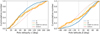 |
Fig. 4 Spin obliquities and pole ecliptic latitudes within various populations. Left panel: cumulative distribution of obliquities for JTs (orange) and of planetesimals obtained in our simulations of the streaming instability (SI) model (blue). The thick orange line corresponds to the nominal spin state solutions, while the thin orange lines represent the spin states based on the bootstrapped photometric datasets. The spins in SI are predominantly prograde with ≃75% having obliquity ε < 90°. We also plot the cumulative distributions for randomly oriented spins (red), and large MBAs (green, spin states adopted from DAMIT). Right panel: same but now for the ecliptic latitude of the rotational pole instead of the spin obliquity. |
4.6 Shape models
We also analyze the shape models of JTs and make a comparison with the population of MBAs. The convex shape models can be best characterized by the ratios of dimensions (a′, b′, c′) along the main axes. We compute the relative dimensions (shape models are not scaled in size) by the “overall dimensions” method of Torppa et al. (2008) and normalize them such that c′ = 1. We note that the c′ dimension is usually the least accurate. In Fig. 5, we plot the a′/b′ vs. b′/c′ axis ratios of JTs, and of large MBAs (D > 30 km in this case), and the dependence of a′/b′ ratio on the size D. We used the shape models of MBAs available in DAMIT and included only those having at least ten optical light curves, thus the most realistic solutions. According to the two-sample Kolmogorov-Smirnov test, the a′/b′ distributions are different (p-value = 10−6), while the b′/c′ distributions are similar (p-value = 0.14). We note that the two-sample K–S test does not depend on the binning of the data.
The bootstrapping described in Sect. 4.3 simultaneously provides shape models that we used for assessing the uncertainties of the ratios of dimensions along the main axes. For each asteroid, we obtained ten bootstrapped shape models for each pole solution. Out of 79 asteroids, only seven have relative uncertainties in a′ larger than 20% and 22 larger than 10%. Similarly, only four asteroids have relative uncertainties in b′ larger than 20% and 24 larger than 10%. This means that the JT population has a rather stable distribution of a′/b′ and b′/c′ axis ratios considering the uncertainties in the dimensions, and thus the statistical tests above should be statistically meaningful.
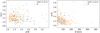 |
Fig. 5 Shape properties within JTs and large MBAs. Left panel: the a′/b′ vs. b′/c′ axis ratios of JTs, and of large MBAs (D > 30 km). Right panel: the a′/b′ ratio as a function of diameter D for the same populations. |
4.7 Assessing the systematic uncertainties by using assumed shapes
As we aim above to compare the obliquity and axial ratio distributions in a quantitative manner, we also need to understand the possible effects of systematic uncertainties in the modeling assumptions on these distributions. In Sect. 4.3, we test the sensitivity of the shape models and spin states on the photometric datasets (by bootstrapping the optical light curves), but under the same model assumptions. Therefore, these uncertainties represent only a lower bound of the total uncertainties. We admit that fully accessing the total uncertainties in the shape models and rotation state parameters requires a robust synthetic study, where various sources of systematic errors should be investigated (noise in data, observing geometries, shapes, spin-state distributions, amount of data, modeling assumptions, inversion method, etc.). This is largely beyond the scope of this work and we leave it for future efforts. However, some selection effects were already quantified in our previous study through a small-scale synthetic study (Hanuš et al. 2011) and the mathematical stability of the convex inversion method for well-formed data sets is well manifested in the literature (e.g., Kaasalainen & Torppa 2001; Kaasalainen et al. 2001).
Here, we decided to assess whether the original shape itself affects the pole-latitude distribution and how well the axis ratios are preserved. Therefore, we performed the following exercise. We assumed that each asteroid in our final sample of solutions has an assumed fixed-shape model – we selected the noncon-vex shape models of asteroids (433) Eros (PDS, 433 Eros Plate Model MSI 1708) and (3) Juno (Viikinkoski et al. 2015). For each asteroid, we used its derived spin state (Table B.2) and the assumed “fake” shape model to generate the new set of optical light curves corresponding to the original epochs. We added noise to each light curve according to its original rms. Then, we derived the spin state and the shape model based on the generated light curve dataset. Finally, we constructed in Fig. A.1 the cumulative obliquity distributions and the axis ratios for each “fake-shape” dataset to assess their stability.
The shapes of Eros and Juno represent substantially different bodies. While Eros is highly elongated and largely concave, Juno is rather round without large concavities. Thus, our exercise covers two end members of the asteroid population. However, we note that JTs should have shapes qualitatively more similar to Juno than Eros. In both cases, the cumulative distribution of obliquities is similar to that of the JTs from Sect. 4.5. This means that the spin vectors were preserved almost independently on the assumed shape model. Only, in the case of Juno, fewer unique solutions were derived, likely because the original models were more elongated, thus with larger imprints in the light curves. This smaller Juno sample still has a similar cumulative obliquity distribution to that of JTs, thus the missing solutions do not have preferential obliquities. The axis ratios of Juno and Eros synthetic JT populations are well preserved, and most of the solutions cluster within 10% in a′/b′ and b′/c′ (Fig. A.1). Such uncertainties are comparable to those assessed by the bootstrapping of the optical data in Sect. 4.3. We note that the dimensions of the original concave shape of Eros lie outside the Eros JTs cluster having higher b′/c′ and borderline a′/b′. The main reasons are the peculiar shape of Eros and its qualitative difference from the convex approximation. The main takeaway from this analysis is that (i) the shape dimensions are relatively well preserved, and (ii) there is no indication of overestimated a′/b′ ratios (the population of JTs has larger a′/b′ ratios than the larger MBAs (D > 30 km), probably not due to the above-analyzed systematic uncertainty).
5 Spin vectors of planetesimals in the streaming instability model
In this Section, we return to the issue of the possible asymmetry between a prograde and retrograde sense of JTs rotation. We first determine what obliquity distribution is expected among the planetesimals born in the trans-Neptunian disk prior to their capture into the JT population. We adopt the currently leading model of planetesimal formation mechanism, namely the streaming instability (SI) in a cold proto-planetary disk.
Streaming instability is a mechanism to aerodynami-cally concentrate small particles in a proto-planetary disk (Youdin & Goodman 2005). Here we analyze the results of 3D simulations of the streaming instability reported in Nesvorný et al. (2019, 2021) and Li et al. (2019). The simulations accounted for the hydrodynamic flow of gas, aerodynamic forces on particles, backreaction of particles on the gas flow, and particle self-gravity. They were performed with the ATHENA code (Bai & Stone 2010). The obliquity distribution of particle clumps in the ATHENA run A12 was reported in Nesvorný et al. (2019). It shows an 80% preference for prograde rotation, which matches the observed distribution of binaries in the Kuiper belt. We performed additional integrations for selected clumps, where we followed their gravitational collapse into individual planetesimals, to understand the implications for the spin states of JTs.
Gravitational collapse of particle clouds was followed with a modified version of the N-body cosmological code PKDGRAV (Stadel 2001), described in Richardson et al. (2000). PKDGRAV is a scalable, parallel tree code that is the fastest code available to us for the proposed simulations. A unique feature of the code is the ability to rapidly detect and realistically treat collisions between particles. The ATHENA simulations were used to set up the initial conditions for PKDGRAV. In total, we performed simulations for 10 representative clumps from A12 (see Nesvorný et al. 2021). Five simulations were completed in each case, where we used slightly modified initial conditions to understand the statistical variability of the results.
All planetesimals with diameters D > 25 km that formed in the PKDGRAV simulations were identified, 103 bodies in total. For each of them, we computed the orientation of the spin vector relative to the reference frame. Since the reference frame of PKDGRAV simulations is set such that the X-Y plane is perpendicular to the initial angular momentum of the cloud, the colatitude of the spin vector gives us the obliquity distribution of planetesimals relative to the clump’s initial angular momentum vector. Finally, we convolved the two distributions to generate predictions for the obliquity distribution of planetesimals with respect to the Solar System plane. Figure 4 shows the result.
There is a notable ≃75% preference for prograde spin, which is similar to predictions of the streaming instability for the orbital inclinations of Kuiper belt binaries (compare with Fig. 3 in Nesvorný et al. 2019). Here, the preference is slightly weaker, 75% vs. 80%, probably because individual objects experienced stochastic growth during gravitational collapse, smearing the initially stronger preference for prograde rotation (binaries preserved it better). Indeed, we see in the PKDGRAV simulation that the spin vectors of individual objects can significantly change during the collapse. For comparison, from the analysis of light curves in this work, we find that JTs show a weaker, ≃60% preference for prograde rotation (Sect. 4.5). There are several options to reconcile these results. For example, as JTs evolved collisionally prior to their capture (e.g., Nesvorný et al. 2018), the initial distribution of obliquities could have been partially randomized. We do not perform any collisional simulations in this paper. The results of collisional simulations depend on many unknown parameters, such as the overall excitation of orbits in the planetesimal disk, momentum transfer in subcatastrophic collisions, or the lifetime of the disk prior to the onset of planetary instability. We thus defer quantitative modeling of these processes to future work.
Apart from the general preference for prograde spins, our numerical simulations of the streaming instability also predict the distribution of planetesimal obliquities that can be compared to the observed obliquity distribution of JTs (Fig. 4). There are some significant differences between the two distributions. The observed obliquity distribution is, in general, wider than the simulated one. It closely follows the model distribution for ε < 50° and starts diverging from it for ε > 50°. We present a more quantitative comparison in Sect. 7.
For completeness, we also analyzed the distribution of the ecliptic latitude ß of the pole for the model and the different observed populations in the right panel of Fig. 4. In the model case, the transformation is trivial: because of the initial cold planetesimal disk, the obliquity is simply 90° – ß. However, the transformation is not so simple for MBAs and JTs. This is because the orbital inclinations extend to large values up to ≃40°. For JTs, the inclinations were excited prior to and during their capture by gravitational perturbations from planets (and possibly other massive objects in the planetesimal disk). It is not exactly known whether, or to what degree, the spins of the captured JTs followed this excitation. So considering both the obliquity and the ecliptic latitude distributions we cover both extreme possibilities: (i) a complete binding of the spins to the orbits during the excitation process, or (ii) spins not being affected by processes that excited the orbital planes. While understanding this issue in detail may again require a complex model, data shown in Fig. 4 luckily manifest that conclusions are the same, independently of whether obliquity or the pole latitude is used. In order to bring quantitative evidence, we tested the corresponding obliquity and ecliptic latitude samples (i.e., for JTs, and DAMIT D > 100 km) by the standard two-sample Kolmogorov-Smirnov test. In both cases, the samples are consistent with being drawn from the same distribution. For instance, the K-S test for the two JTs samples (i.e., obliquities vs. ecliptic latitudes) gives p-value = 0.09.
6 Post-capture spin evolution
In this section, we consider what happens to the Trojan spin state during the long period of time after they have been captured in the coorbital state with Jupiter. We consider dynamical, rather than collisional effects in this section. This is because we assume that the collisional activity among Trojan clouds after the capture was dwarfed by a much more intense period before capture. Given the commonly accepted point of view, the capture happened during the early evolution of the Solar System (possibly 4.4–4.5 Gyr ago or so; e.g., Nesvorný 2018), when giant planets underwent a chaotic reconfiguration terminated by Jupiter’s inward jump to near its current orbit (e.g., Nesvorný et al. 2013). Planetesimals roaming in the planet-crossing zone that happened to be suitably situated with respect to the Jupiter orbit at that moment formed the early Trojan population. The implication of this model is the marginal stability of a fraction of the Trojan population such that over eons that followed about 23% of them leaked away (e.g., Holt et al. 2020), leaving even some of the currently observed Trojans on unstable orbits ready to escape from the population in the close future (Sect. 6.3). Even some of the Trojans residing currently stable orbits (that will stay in the population for another gigayear), might have underwent orbital evolution since their origin due to subtle chaoticity in their orbital phase space. As a result, it is not our aim to describe in detail the past gigayear-lasting evolution of spin state even for our limited sample of 90 Trojans, for which we know it today, as this is a task that is too difficult.
Instead, we probe the shorter-term evolution of the Trojan spin state and consider it an operational proxy of what happens on longer timescales. In particular, we propagate, using the model described in Sect. 6.1, the spin states of our sample of Trojans for 50 Myr forward in time. Note this is information equivalent to the propagation backward in time. Given the main arguments in this paper (Sect. 4.5), we are principally interested to know whether there is a substantial evolutionary flow of Trojan spins between the prograde- and retrograde-rotating groups. Finding there is little of such interchange on the monitored 50 Myr time interval, we dare to extrapolate the conclusion to gigayear-long evolution.
6.1 Dynamical model
Assume the body rotates about the axis of the largest inertia tensor. If no torques are applied, the rotational angular momentum L is conserved. This implies that both (i) the angular rotation rate ω, and (ii) the unit vector s of the rotation pole in the inertial frame are also constant. However, if we aim to know what happens to the Trojan rotation state over a long period of time, we need to include relevant torques of which the most important are due to the gravitational effects of the Sun and planets (the radiation-related YORP torques would have been important only for timespan exceeding ≃5 Gyr for D < 40 km Trojans, e.g., Vokrouhlický et al. 2015). Each of the perturbing bodies may be represented by a point source of mass M and its gravitational field expanded in the local frame of the Trojan to the quadrupole level. Assuming the origin of the local frame coincides with the center-of-mass of the Trojan, the rotation-averaged gravitational torques may be expressed in simple terms as (e.g., Colombo 1966; Bertotti et al. 2003, Chap. 4)
![Mathematical equation: ${\bf{T}} = - {{3GM} \over {{r^5}}}\left[ {C - {1 \over 2}\left( {A + B} \right)} \right]\left( {{\bf{s}} \cdot {\bf{r}}} \right)\left( {{\bf{s}} \times {\bf{r}}} \right),$](/articles/aa/full_html/2023/11/aa46022-23/aa46022-23-eq6.png) (5)
(5)
where G is the gravitational constant, r position vector of the Trojan with respect to the source (r = |r|), and (A ≤ B ≤ C) are the principal moments of the inertia tensor. Because L = Cωs in the principal axis rotation state, the Euler equation dL/dt = T implies that ω is conserved in this approximation. However the pole direction s evolves according to
 (6)
(6)
where ![Mathematical equation: ${\rm{\Delta }}\,{\rm{ = }}\,{{\left[ {C - {1 \over 2}\,\left( {A + B} \right)} \right]} \mathord{\left/ {\vphantom {{\left[ {C - {1 \over 2}\,\left( {A + B} \right)} \right]} C}} \right. \kern-\nulldelimiterspace} C}$](/articles/aa/full_html/2023/11/aa46022-23/aa46022-23-eq8.png) is the dynamical flattening. For nearly spherical objects ∆ is very small, and it reaches maximum values near to 0.5 for highly irregular-shaped bodies. Contributions from different massive bodies in the Solar System linearly superpose on the righthand side of Eq. (6).
is the dynamical flattening. For nearly spherical objects ∆ is very small, and it reaches maximum values near to 0.5 for highly irregular-shaped bodies. Contributions from different massive bodies in the Solar System linearly superpose on the righthand side of Eq. (6).
In our most complete simulations, we included the Sun and Jupiter as sources of the gravitational torques. In this approach, we numerically integrated Eq. (6) using a simple Euler scheme and a short timestep of 3 days. The value of the rotation frequency ω was obtained from our solution of the rotation period, and the dynamical flattening ∆ from the nominal shape of the body and assumption of a homogeneous density distribution (see, e.g., Dobrovolskis 1996). We embedded this unit into a general-purpose orbit-propagation package swift_rmvs4, which provided the position vectors r for each of the sources (and used the same timestep of 3 days for the orbit integration). All planets, and the Sun, were propagated using swift_rmvs47, together with our sample of Trojans for which rotation states were inferred in Sect. 4. The planetary and Trojan heliocentric position vectors were integrated in a global reference frame defined by the invariable plane of the Solar System. For that reason, we also transformed Trojan pole directions s into the same system at the beginning of the integration. The corresponding tilt is, however, very small, as the ecliptic plane has an inclination of only ≃1.5° to the invariable plane. Therefore the pole latitudes differed in the two systems at maximum by this value. We performed the simulations forward in time over 50 Myr interval, over which most of the orbits were stable (see though Sect. 6.3 for more comments).
In our first set of integrations, we included the gravitational torque due to Jupiter’s gravity on the righthand side of Eq. (6) for the sake of completeness and also for its special status with respect to the Trojan clouds. However, we found that its effect is minimal over the timescale of 50 Myr we considered (a result that likely would not change even over a longer timescale). This is because the Solar torque is much more significant owing to its much larger mass (in spite of the fact that some Trojans with large libration amplitude in our sample may approach Jupiter at a distance that is slightly more than half of the Solar distance). We thus find that adequate results can be obtained when considering the Solar gravitational torque only on the righthand side of Eq. (6). This model has further important advantages.
First, we observe that the secular changes of s have periods comparable with that of the precession of the Trojan orbital plane rather than a much shorter revolution period about the Sun. It is thus possible, and convenient, to further average the torque (Eq. (5)) over the revolution cycle about the Sun. Assuming osculating elliptical orbit, this may be performed analytically using
 (7)
(7)
where  is the semiminor axis of the elliptic orbit (a and e being the respective semimajor axis and eccentricity), E is the unitary 3 × 3 matrix and n is the unit vector normal to the osculating orbital plane in the direction of the orbital angular momentum. Therefore, nT = (sin I sin Ω, − sin I cos Ω, cos I), where I is the orbit inclination to the reference plane and Ω is the longitude of the node. As a result, Eq. (6) now takes the form (e.g., Colombo 1966)
 (8)
(8)
where
 (9)
(9)
is the precession constant. The fundamental difference between Eqs. (6) and (8) is that none of the parameters on the righthand side of the latter changes on the timescale of Trojan’s orbital revolution about the Sun (neglecting very small short-period changes in the semiminor axis b in the definition of the precession constant α). Therefore, Eq. (8) may be numerically integrated with a much larger timestep, obtaining results quite more efficiently. In our simulations, we used a 50 yr timestep, instead of the 3 day timestep needed for integration of Eq. (6). Additionally, Breiter et al. (2005) developed an efficient symplectic scheme for the propagation of Eq. (8), which conveniently conserves its first integrals. We implemented their LP2 scheme. The knowledge of the orbital evolution is still needed, as the normal vector n changes its direction in the iner-tial space due to the orbit precession and inclination variations (that is, both I and Ω are time-dependent due to planetary perturbations). In order to fully describe both, we still use the orbital integration by swift_rmvs4 package and include the Trojan spin integrator of Eq. (8) as a separate subunit of the code.
Second, a great advantage of using the second model described by Eq. (8) consists of the fact that its solutions have been thoroughly studied since Colombo (1966). This past and well-known analysis provides a key insight into why some of the Trojan pole solutions exhibit only very small variations of the pole latitude, while in other cases large variations of the latitude are possible. Importantly, while many perturbations, reflecting planetary orbits and their own evolution, participate in the time evolution of Trojan orbital n vector, not all are equally prominent. In fact, the evolution of n is nearly always dominated by a contribution from a single, proper term. In this case, the inclination I is constant and the longitude of the node exhibits a steady precession with the proper frequency s (thus Ω = st + Ω0). In this simplified model, called the Colombo top (e.g., Colombo 1966; Henrard & Murigande 1987), the variety of solutions of Eq. (8) depends on three parameters: (i) the two frequencies α and s, and (ii) the orbit inclination I. The complexity stems from the possibility that α and s enter in a resonance. As a result, the flow of s on a unit sphere has two distinct regimes according to the ratio κ = |α/s| (our notation adopted here, recalling that α is positive and s negative, may differ from the signature in other references). When, κ < κ⋆, where κ⋆ = (sin2/3 I + cos2/3 I)3/2, s exhibits a simple circulation about two fixed points called Cassini state 2 and 3. In the limit of very small κ value, these stationary points have obliquity of I and 90°−I. The spin vector s thus circulates about the north or south poles of the invariable frame in the inertial system, and the rotation pole latitude has only small variations. A more complex regime onsets when κ > κ⋆ (note that κ⋆ ranges between the value 1 at very small inclination and reaches a maximum of 2 when I = 45°). In this situation, the flow of s navigates between four fixed points, called Cassini state 1 to 4. Cassini states 2 and 4 are stable and unstable stationary points of a resonant zone. The appearance of this zone triggers large obliquity oscillations, which are then reflected by large oscillations of the rotation pole latitude. Transitions between the prograde and retrograde rotation regimes are in principle possible. Mathematical details of the Colombo top problem may be found in a number of publications (e.g., Colombo 1966; Henrard & Murigande 1987; Haponiak et al. 2020).
We need to decide on which of the two regimes is to be expected more typical for Trojan spin evolution. For small eccentricities, we may adopt b ≃ a ≃ 5.2 au in the Trojan region, and thus α ≃ 9.4 ∆ (P/6 h) arcsec yr−1 (seeEq. (9)). Additionally, the population of large Trojans we are interested in has rather regular shapes, typically with ∆ ≃ 0.1–0.2. As a result, the precession constant values are typically ~arcsec yr−1 unless the rotation period P is long (several tens of hours or so). In the same time, the proper frequencies s have values typically in the range −5 to −30 arcsec yr−1, and only exceptionally have a value smaller (e.g., Milani 1993). As a result, the situation we should encounter most often among Trojans is the limit of very small κ, implying thus only small variations of the rotation pole latitude. Exceptions are to be expected when the rotation period P is very long, and/or proper frequency s is anomalously small.
Results from our simulations confirm these conclusions. Tables 1 and 2 provide results from simulations where we propagated all our pole solutions from Sect. 4 for 50 Myr interval to the future. We used the most complete torque model, including both the Sun and the Jupiter effects in Eq. (6), although the results from the secular model using Eq. (8) are nearly identical. We were mainly interested in the behavior of the rotation pole latitude, as this parameter helps us classify Trojans into prograde- and retrograde-rotating groups. The columns b0 give the initial latitude in the invariable-frame reference system. For each body we propagate both pole solutions P1 and P2; only in cases, for which the pole solution is unique, we have just the P1 data. The columns denoted bmin and bmax give minimum and maximum latitude values attained over the monitored 50 Myr time interval. In most of the cases, the latitude variations are very small, reflecting a large separation between α and s frequencies. The rotation of these bodies is well represented by the κ≪κ⋆ solutions of the Colombo top. Importantly, this majority of Trojans thus remain safely within their group, either prograde or retrograde rotators, and do not confuse our conclusions by possible transitions between them. As anticipated, in a few cases we observe a larger range of variations in the pole latitude. Here, κ≃κ⋆ or even κ>κ⋆ for either of the two reasons mentioned above. The pole solution may still remain in its category, but in exceptional cases, it may even temporarily transition between prograde- and retrograde-rotating categories (in Sect. 6.2, we illustrate three of such cases in some detail). The overall balance of this flow is excepted to be directed toward retrograde states, helping slightly to solve the difference between the observed JT spin states and the modeled original spins (Sect. 5). This is because the Cassini resonance is predominantly located in the prograde rotation zone.
6.2 Trojans with large variations of pole latitude
In this section, we illustrate reasons for large latitude variations of the rotation pole for three exceptional Trojans. We start with the pole solution of (1867) Deiphobus, the L5 cloud member, for which we predict the largest effect in this group (see Table 2). In this case, the orbit has a proper inclination I ≃ 28.3° and proper frequency s ≃ −6.23 arcsec yr−1. Our estimated ∆ ≃ 0.246 from the shape model and rotation period P ≃ 59.18 h provide α ≃ 21.86 arcsec yr−1. As a result, we have κ ≃ 3.509 and κ⋆ ≃ 1.886. Thus κ > κ⋆, principally due to the very slow rotation of Deiphobus and the resonant situation with four Cassini states apply. The obliquity ε2 of the resonant center, the Cassini state 2, is among the solutions of the equation of κ sin 2ε2 = 2 sin(ε2 − I) (e.g., Colombo 1966). Interestingly, this quartic equation may be solved analytically (e.g., Haponiak et al. 2020), providing ε2 ≃ 77.2°, quite larger than the proper inclination value. Because of the large proper inclination I and proximity of κ to κ⋆ the resonant zone occupies a large portion of the phase space: it spans from ≃28.9° to ≃117.1° in obliquity along the ϕp = 0° section. Finally, the present-date obliquity value of our unique pole for Deiphobus is ≃37°, not too close to the Cassini state 2. This implies that while circulating about the Cassini state 2, Deiphobus pole obliquity will exhibit large oscillations and these will be reflected in large variations of the pole latitude in the inertial frame.
Data shown on Fig. 6 confirm these conclusions. While the estimates mentioned above used the simplified Colombo top model, the solution shown here is obtained by full-fledged numerical simulations. Its closeness to what the Colombo model predicts justifies its validity. In particular, the top panel shows osculating obliquity as a function of time over 2 Myr initial segment of our simulation. The large-amplitude oscillation with a period of ≃243 kyr is the projected circulation about the Cassini state 2. To see the effect more fully, we also transformed the s evolution into the variables defined in the proper-term orbital frame (that is, the frame having the reference plane inclined by the proper orbital inclination value and precessing in the inertial frame with exactly s frequency): (i) the proper obliquity εp, namely the angle between s and the z-axis of the proper frame, and (ii) the proper longitude ϕp, namely the angle between the s projected onto the reference proper plane and the x-axis rotated 90° away from the proper node. The Cassini state 2 is shown by the red dot at ϕp = 0°, and the gray curves are exact solutions of the idealized Colombo top model (e.g., Haponiak et al. 2020). The true s evolution in these variables follow very closely the neighboring gray lines justifying the approximate validity of the Colombo model. The takeaway message is that the large obliquity oscillations, between ≃35° and ≃113°, are indeed triggered by oscillations about the Cassini state 2, which itself is tilted to a large ε2 value8.
The resonant zone about the Cassini state 2 is predominantly located in the prograde rotation zone, but its presence may considerably affect solutions in the retrograde rotation zone. An example of this behavior is the L4 member (15663) Periphas (see Table 1). In this case, our solution yields ∆ ≃ 0.233 and the rotation period P ≃ 9.92 h, not suspiciously large. Together with other orbital parameters, they provide a rather small value of the precession constant α ≃ 3.54 arcsec yr−1. However, the really small value of the orbital precession frequency (partly due to large inclination value I ≃ 33.94°), s ≃ −1.61 arcsec yr−1, makes this case anomalous. We thus obtain κ ≃ 2.20 and κ⋆ ≃ 1.95. The proximity of κ to κ⋆ implies the resonant zone about the Cassini state 2, here at ε2 ≃ 72.6°, is large. This is demonstrated at the bottom panel of Fig. 6. However, the rotation of Periphas is retrograde, with the current obliquity value of ≃142°, and it does not interact with the Cassini resonance directly. The evolutionary track of the Periphas’ spin evolution is shown on Fig. 6 confirms it circulates about the Cassini state 3. Still, the Cassini resonance reaching up to obliquity of ε ≃123° pushes even the retrograde solutions to perform large obliquity variation, nearly 30° as shown in the upper panel of Fig. 6.
In order to demonstrate that the existence of the Cassini resonant zone is not a necessary condition for large latitude oscillations we consider (4834) Thoas, another L4 Trojan (Table 1). In this case, the proper inclination has a value I ≃ 27.05° and the proper frequency s ≃ −4.58 arcsec yr−1. The rotation period is not suspiciously long, P ≃ 18.19 h, and thus the precession constant is rather low α ≃ 6.20 arcsec yr−1. As a result κ < κ⋆ in this case, but not much smaller due to the moderately small value of the proper frequency s and moderately long rotation period (κ ≃ 1.35, while κ⋆ ≃ 1.87). There are only two Cassini states, but due to the proximity of κ to κ⋆ the Cassini state 2 is forced to already a large obliquity value of ε2 ≃ 61.6°. Figure 7 illustrates the whole situation and also shows Thoas’ spin evolution over the next 2 Myr interval starting with our unique pole solution. The bottom panel shows a projection of the spin evolution into the phase-space variables of the Colombo model associated with the proper variables. The spin axis of Thoas performs a slow circulation about the Cassini state 2 shifted to an anomalously large value of the obliquity. This evolution then triggers a large amplitude of Thoas’ obliquity oscillations, also reflected in large latitude excursions.
The takeaway message from this section is that all cases for which the polar latitude was found to oscillate in a large interval of values in our numerical simulations (Tables 1 and 2) may be understood using the Colombo top model. They correspond to the situations when κ is not much smaller than κ⋆, therefore when the Cassini resonance exists of is about to emerge. Due to the typically large proper inclination of Trojan orbits, the Cassini resonance zone occupies a large portion of the phase space and drives large obliquity oscillations.
Limits of oscillations of the rotation pole latitude for L4 Trojans.
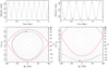 |
Fig. 6 Results from a short-term integration of the rotational pole direction s for the L5 Trojan (1867) Deiphobus (left panels) and for the L4 Trojan (15663) Periphas (right panels). The top panel shows the osculating obliquity as a function of time. The bottom panel provides a projection of the s evolution over the 2 Myr timespan onto the phase space defined by the proper-frame variables: (i) obliquity εp on the ordinate, and (ii) longitude ϕp at the abscissa. The numerically integrated evolution is shown by a black line with the initial conditions shown by the blue diamond. The gray lines are idealized flow-lines from the simple Colombo top model. Red line is the separatrix of the resonant zone, and red points are locations of the Cassini state 2 (the Cassini state 4 is at the junction of the two separatrix branches with ϕp = ±180°). |
6.3 Unstable Trojans
For completeness, we also comment on orbital stability for Trojans in our sample with resolved rotation poles. In most cases, their orbits were fairly stable over the interval of 50 Myr used for monitoring the variations of the pole latitude. But in five cases we noticed orbital instability onset even during this period of time. Here we report only those deemed “macroscopically unstable”, in which orbital eccentricity or inclination exhibited large jumps, and we omit cases exhibiting traces of only “stable chaos” on the 50 Myr timescale.
Analysis of the Trojan cloud stability has a long history, and it is not our goal to provide a comprehensive review here. The observed population analysis (as opposed to purely mathematical studies) was provided by Milani (1993), who computed synthetic proper elements of a set of 174 Trojans based on a megayear-long numerical integration. Some 13% of these orbits showed various traces of instability evidenced by the Lyapunov timescales between 60 and 600 kyr. This sample of chaotic orbits was later studied in more detail using numerical integrations spanning a longer timescale of 50 to 100 Myr (e.g., Pilat-Lohinger et al. 1999; Dvorak & Tsiganis 2000; Tsiganis et al. 2000). These studies helped to describe macroscopic orbital instability and identified the associated dynamical reasons. Even longer, the gigayear timescale orbital stability of Trojans was studied by Levison et al. (1997), as afforded by development in symplectic numerical tools. These authors estimated that some 12% of real Trojans escape over the Solar System age from their population. This fraction was recently even increased to about 23% by Holt et al. (2020), perhaps by using data for many more, especially small Trojans. Overall, the nearly steady leakage of even large Trojans may be understood by realizing their formation mechanism that allows them to fully fill their phase space up to limits of instability (e.g., Nesvorný et al. 2013). Finding that few of our studied 90 Trojans reside on noticeably unstable orbits is therefore not surprising.
Figure 8 shows results from our simulations of two macro-scopically unstable Trojans in our sample: (i) (1868) Thersites (left), and (ii) (5144) Achates (right)9. Especially the large eccentricity Achates’ orbit indicates macroscopic chaos witnessed here by irregular evolution of the inclination (top panel on Fig. 8; see also Dvorak & Tsiganis 2000) due to intermittent interaction with several secular resonances (of which ν16 is the most prominent). In fact, we numerically propagated the nominal orbit of (5144) Achates together with 49 very close orbital clones (all starting from the uncertainty interval of its currently determined orbit) for 1 Gyr forward in time. We found that a median timescale before ejection from the Trojan region was ≃220 Myr, in good agreement with the data in Fig. 1 of Levison et al. (1997), and comparable to the case of yet another unstable Trojan (1173) Anchises (see Horner et al. 2012). Similarly, (1868) Ther-sites is a well studied unstable orbit (left panel; see Tsiganis et al. 2000). In our simulation, the inclinations instability onsets at ≃44 Myr. In both cases, however, the orbital instability has little effect on the rotation pole latitude (bottom panels on Fig. 8 where we used the P1 solution for both Trojans). This is because both objects have sufficiently short rotation periods, such that always κ ≪ κ⋆ during the integrated time interval. As a result, the unstable nature of the Thersites and Achates orbits does not seem to confuse our conclusions as far as the rotation pole categories (prograde or retrograde) are concerned.
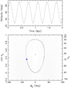 |
Fig. 7 Results from a short-term integration of the rotational pole direction s for the L4 Trojan (4834) Thoas. The top panel shows the osculating obliquity as a function of time. The bottom panel provides a projection of the s evolution over the 2 Myr timespan onto the phase space defined by the proper-frame variables: (i) obliquity εp on the ordinate, and (ii) longitude ϕp at the abscissa. The numerically integrated evolution is shown by a black line with the initial conditions shown by the blue diamond. The gray lines are idealized flow-lines from the simple Colombo top model. Red point marks the location of the Cassini state 2. |
7 Discussion
The axis ratios of JTs with shape models are formally compatible in b′/c′ and incompatible in a′/b′ with the population of larger (D > 30 km) MBAs. JTs contain less near-spherical and more elongated bodies than the sample of MBAs. There are, however, several caveats concerning the JTs. Namely, (i) the number of objects is rather small compared to MBAs (90 vs. 218), (ii) the axis ratios have large uncertainties in cases where the shape models are based on limited photometric datasets, and, in general, concerning the c dimension, (iii) the sample is biased toward objects with larger amplitudes, thus we likely miss (oblate) spheroids. Therefore, it is difficult to conclude whether the shapes are indeed similar within the two populations. The open question here is whether oblate spheroids dominate in the JT population, which might indicate the lesser importance of collisions since their formation. We do not see many in our sample, which is a common property with MBAs. However, we already learned an important lesson about the bias in the main belt concerning oblate spheroids. Only recently, the shape models or large asteroids of (10) Hygiea, (31) Euphrosyne, (324) Bam-berga, or (702) Interamnia were derived thanks to disk-resolved images from the high-resolution SPHERE instrument mounted on the 8 meter-class Very Large Telescope (Vernazza et al. 2020, 2021; Yang et al. 2020; Hanuš et al. 2020). All these asteroids have shapes consistent with an oblate spheroid and have not been derived before using optical photometry only (thus no previous convex shape models). It is likely that the difficulty in deriving the shapes of such bodies applies to JTs as well.
In our study, we focus on testing whether the observed physical properties of JTs are consistent with those predicted based on the currently most acceptable formation scenario – capture to their current orbits near the Lagrangian points of Jupiter during the early reconfiguration of the giant planets from the planetes-imals born in the massive trans-Neptunian disk. The numerical simulations of the streaming instability, the leading mechanism for the planetesimals formation, predict the spin obliquity distribution and the ratio between the number of prograde and retrograde rotators. Both predictions are testable by observed properties. The streaming instability predicts a somewhat larger fraction of prograde rotators than we observe (75% vs. 60%). However, this could be attributed to, for example, (i) partial randomization due to collisional evolution prior to the capture, or (ii) due to post-capture collisional and orbital evolution. We modeled the latter mechanism in Sect. 6 and showed that it can be responsible for some minor depletion of prograde rotators.
In Sect. 5, we consider only planetesimals with D > 25 km. This limit corresponds to the absolute magnitude of H ~ 12 mag (assuming a geometric visible albedo of pV = 0.05). Thus, we limit our JT sample to objects with H ≤ 12 mag for the analysis of the pole obliquities. This limit also conveniently excludes objects whose obliquities could be affected by YORP thermal forces. Although YORP is weaker for JTs than for MBAs given the difference in the distance from the Sun, the size at which it is important is roughly the same for the two populations. This is due to the JTs having significantly longer collisional lifetimes than similarly sized MBAs. Considering JTs smaller than ~25 km in the spin vector analysis could affect our interpretations as those spin vectors could be significantly evolved by the YORP.
In Fig. 4, we compare the obliquity distributions of several populations, including JTs, and of the prediction based on streaming instability (SI). The obliquity distribution of JTs seems to be visually the closest match to the SI distribution, however, the K–S test does not support the hypothesis that the two samples are drawn from the same distribution (p-value = 0.015). Indeed, JTs lack members with obliquities in the interval 50°–70° and contain more retrograde bodies. As discussed earlier, several dynamical processes could affect the distribution. In addition, the observing bias should be present as well. The shape and spin solutions are derived by the convex inversion method and it was shown by Hanuš et al. (2011) that objects with obliquities near 0° and 180° are derived more successfully than bodies with obliquities near 90°, namely even by 30–40%. This is because the former bodies lack the pole-on observing geometry, which provides only low-amplitude brightness changes often comparable to the noise scatter. By correcting the observed obliquity distribution on this bias, we would obtain more objects with mid-value obliquities and thus a better agreement with the SI distribution. However, the excess of retrograde rotators would still exist. Interestingly, the obliquities of JTs and large main-belt asteroids are the most similar (although inconsistent) with the KS test p-value = 0.02. The main difference is for small obliquities (ε < 50°).
Although the observed sample of JT obliquities is still rather small, the comparison with the streaming instability predicted obliquities suggests that this formation scenario could be consistent with the observed properties of JTs. The main issue is the overabundance of retrograde rotators with ε > 130°.
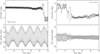 |
Fig. 8 Two orbitally unstable Trojans: (i) L4 object (1868) Thersites in the left panels, and (ii) L5 object (5144) Achates in the right panels. The top panels show time dependence of the osculating orbital inclination with respect to the invariable plane. Bottom panels show the evolution of the pole P1 latitude in the same reference system. |
8 Conclusions
Deriving physical properties of JTs is challenging due to various obstacles – the observing geometry is changing much slower than for MBAs and is limited to phase angles (i.e., angle Sun-asteroid-Earth) up to just a few degrees; their large distance to the Earth together with their low albedo makes them rather faint objects accessible to at least meter-class telescopes. Therefore, their photometry is scarce and often affected by large uncertainties. Despite that, the currently available photometric datasets can be successfully used for the physical characterization of several tens of JTs.
By analyzing optical datasets for ~1000 JTs, we obtained spin state and shape solutions in 79 cases (Sect. 4). We found that the observed distribution of the pole obliquities/latitudes of JTs is broadly consistent with expectations from the streaming instability (Sect. 5), which is currently considered the leading mechanism for the formation of planetesimals in the trans-Neptunian disk. Observed JTs latitude/obliquity distribution has a slightly smaller prograde/retrograde asymmetry (excess of obliquities >130°) than that expected from the existing streaming instability simulations. However, this discrepancy can be plausibly reconciled by the effects of the post-formation collisional activity. Our numerical simulations of the post-capture spin evolution in Sect. 6 indicate that the JTs’ pole distribution is not significantly affected by dynamical processes such as the eccentricity excitation in resonances, close encounters with planets, or the effects of non-gravitational forces. However, a few JTs exhibit large latitude variations of the rotation pole and may even temporarily transition between prograde- and retrograde-rotating categories.
As surveys with better accuracy, faster cadence, and higher limiting magnitudes are substituting or supplementing the already established surveys, better data become available. This will lead to an increase in the number of spin state solutions within the JTs, which should increase the significance of our results and possibly reveal hidden dependencies within various physical properties of JTs. Ideally, the larger statistical sample should further constrain theoretical models aiming at explaining the origin of the JT population.
JTs are also commonly targeted by the stellar occultation hunters – the event predictions are now rather accurate leading to many positive detections, which further improves the ephemeris, thus future stellar occultation predictions. Convex shape models, together with the stellar occultation profiles can provide direct measurements of the dimensions, volume, and eventually bulk density if an accurate mass estimate is available (e.g., from system multiplicity). Occultation measurements also provide reliable estimates of axis ratios, which will help to assess whether the shapes of JTs are similar to the shapes of MBAs.
The remote-like studies of physical properties of JTs such as ours represent invaluable support for the insitu exploration of several JTs by the Lucy mission (Levison et al. 2021). Only a combination of both approaches can lead to the most complete understanding of the JT population and, if properly modeled, also the trans-Neptunian population.
Acknowledgements
The work of J.H. and J.D. has been supported by the Czech Science Foundation through grant 22-17783S and by the Erasmus+ program of the European Union under grant number 2020-1-CZ01-KA203-078200. The work of D.V. has been supported by the Czech Science Foundation through grant 21-11058S. The observational work by V. Benishek at the Sopot Astronomical Observatory in Serbia was kindly supported by the Shoemaker NEO Grants from the Planetary Society for 2017 and 2021. The work of P.P. has been supported through a NASA Solar System Workings award number 80NSSC21K0153. This research has used the Minor Planet Physical Properties Catalogue (MP3C) of the Observatoire de la Côte d’Azur and the IMCCE’s Miriade VO tool. We thank Brian A. Skiff from the Lowell Observatory for providing the data for asteroid (5209) 1989 CW1. This work has made use of data from the Asteroid Terrestrial-impact Last Alert System (ATLAS) project. ATLAS is primarily funded to search for near-Earth asteroids through NASA grants NN12AR55G, 80NSSC18K0284, and 80NSSC18K1575; byproducts of the NEO search include images and catalogs from the survey area. The ATLAS science products have been made possible through the contributions of the University of Hawaii Institute for Astronomy, the Queen’s University Belfast, the Space Telescope Science Institute, the South African Astronomical Observatory (SAAO), and the Millennium Institute of Astrophysics (MAS), Chile. We would like to thank our reviewer for taking the time and effort necessary to review the manuscript. We sincerely appreciate all valuable comments and suggestions, which helped us to improve the quality of the manuscript.
Appendix A Additional figures
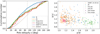 |
Fig. A.1 Assessing the systematic uncertainties by using assumed shapes. Left panel: The cumulative distribution of obliquities for JTs (orange), for synthetic JTs population assuming the shape models of (433) Eros (green) and (3) Juno (red), and of planetesimals obtained in our simulations of the streaming instability (SI) model (blue). We also plot the cumulative distributions for randomly oriented spins (brown), and large (D > 100 km) MBAs (purple, spin states adopted from DAMIT). Right panel: The a′/b′ vs. b′/c′ axis ratios of JTs, of large MBAs (D > 30 km), and of synthetic JT populations assuming the shape models of (433) Eros and (3) Juno. We also indicate the axis ratios for the original shapes of (433) Eros and (3) Juno. |
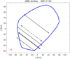 |
Fig. A.2 Projection of the shape model of (588) Achilles. The volume equivalent diameter is 131 ± 8 km. |
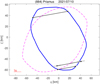 |
Fig. A.3 Projection of the shape model of (884) Priamus. Only the model with the pole (1o,−32°) agrees with the observed chords, its equivalent diameter is 105 ± 4 km. |
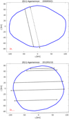 |
Fig. A.4 Projection of the shape model of (911) Agamemnon. The model with the pole (290°, 35°) agrees with the observed chords, its equivalent diameter is 153 ± 6 km. |
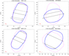 |
Fig. A.5 Projection of the shape model of (1437) Diomedes. Only the model with the pole (147°, 5°) agrees with the observed chords, its equivalent diameter is 133 ± 5 km. |
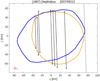 |
Fig. A.6 Projection of the shape model of (1867) Deiphobus. The convex shape model (blue) with the pole (338°, 79°) does not agree well with the observed chords. The nonconvex ADAM model (orange) provides a much better fit with the pole direction (329°, 67°) and an equivalent diameter of 108 ± 4 km. The second chord from the left is not consistent with the two other chords next to it, probably due to some systematic error (or the shape is highly concave at this place). Due to the negative observation (miss chord on the right), the shape cannot be larger and its size is significantly smaller than the values derived from Akari (131 ± 2 km) and IRAS (123 ± 4 km) data. |
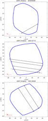 |
Fig. A.7 Projection of the shape model of (2207) Antenor. The model with the pole (86°, −19°) and equivalent diameter of 101 ± 3 km agrees well with the observed chords. |
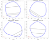 |
Fig. A.8 Projection of the shape model of (4709) Ennomos. The model with the pole (241°, 75°) and equivalent diameter of 91 ± 4 km agrees with the observed chords. |
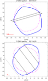 |
Fig. A.9 Projection of the shape model of (31344) Agathon. The model with the pole (112°, 52°) and equivalent diameter of 38 ± 1.5 km agrees with the observed chords better than the second pole solution (294°, 36°) and equivalent diameter of 35 ± 3 km. |
References
- Babusiaux, C., Fabricius, C., Khanna, S., et al. 2023, A & A, 674, A32 [Google Scholar]
- Bai, X.-N., & Stone, J. M. 2010, ApJS, 190, 297 [NASA ADS] [CrossRef] [Google Scholar]
- Barucci, M. A., Cruikshank, D. P., Mottola, S., & Lazzarin, M. 2002, in Asteroids III, eds. W. F. Bottke, A. Cellino, P. Paolicchi, & R. P. Binzel, 273 [CrossRef] [Google Scholar]
- Bellm, E. C., Kulkarni, S. R., Graham, M. J., et al. 2019, PASP, 131, 018002 [Google Scholar]
- Bertotti, B., Farinella, P., & Vokrouhlický, D. 2003, Physics of the Solar System – Dynamics and Evolution, Space Physics, and Spacetime Structure (Dordrecht: Kluwer Academic Press) [Google Scholar]
- Breiter, S., Nesvorný, D., & Vokrouhlický, D. 2005, AJ, 130, 1267 [Google Scholar]
- Chang, C.-K., Chen, Y.-T., Fraser, W. C., et al. 2021, Planetary Science journal, 2, 191 [NASA ADS] [CrossRef] [Google Scholar]
- Colombo, G. 1966, AJ, 71, 891 [Google Scholar]
- De Luise, F., Dotto, E., Fornasier, S., et al. 2010, Icarus, 209, 586 [NASA ADS] [CrossRef] [Google Scholar]
- Dobrovolskis, A. R. 1996, Icarus, 124, 698 [NASA ADS] [CrossRef] [Google Scholar]
- Ďurech, J., Sidorin, V., & Kaasalainen, M. 2010, A & A, 513, A46 [Google Scholar]
- Ďurech, J., Kaasalainen, M., Herald, D., et al. 2011, Icarus, 214, 652 [Google Scholar]
- Ďurech, J., Hanuš, J., & Vanco, R. 2019, A & A, 631, A2 [CrossRef] [EDP Sciences] [Google Scholar]
- Ďurech, J., Tonry, J., Erasmus, N., et al. 2020, A & A, 643, A59 [CrossRef] [EDP Sciences] [Google Scholar]
- Dvorak, R., & Tsiganis, K. 2000, Celest. Mech. Dyn. Astron., 78, 125 [NASA ADS] [CrossRef] [Google Scholar]
- Emery, J. P., Burr, D. M., & Cruikshank, D. P. 2011, AJ, 141, 25 [NASA ADS] [CrossRef] [Google Scholar]
- Emery, J. P., Marzari, F., Morbidelli, A., French, L. M., & Grav, T. 2015, in Asteroids IV, eds. P. Michel, F. E. DeMeo, & W. F. Bottke, 203 [Google Scholar]
- Fornasier, S., Dotto, E., Hainaut, O., et al. 2007, Icarus, 190, 622 [NASA ADS] [CrossRef] [Google Scholar]
- Hanuš, J., Ďurech, J., Brož, M., et al. 2011, A & A, 530, A134 [CrossRef] [EDP Sciences] [Google Scholar]
- Hanuš, J., Vernazza, P., Viikinkoski, M., et al. 2020, A & A, 633, A65 [CrossRef] [EDP Sciences] [Google Scholar]
- Hanuš, J., Pejcha, O., Shappee, B. J., et al. 2021, A & A, 654, A48 [CrossRef] [EDP Sciences] [Google Scholar]
- Haponiak, J., Breiter, S., & Vokrouhlický, D. 2020, Celest. Mech. Dyn. Astron., 132, 24 [Google Scholar]
- Henrard, J., & Murigande, C. 1987, Celest. Mech., 40, 345 [Google Scholar]
- Herald, D., Gault, D., Anderson, R., et al. 2020, MNRAS, 499, 4570 [Google Scholar]
- Holt, T. R., Nesvorný, D., Horner, J., et al. 2020, MNRAS, 495, 4085 [NASA ADS] [CrossRef] [Google Scholar]
- Horner, J., Müller, T. G., & Lykawka, P. S. 2012, MNRAS, 423, 2587 [CrossRef] [Google Scholar]
- Kaasalainen, M., & Lamberg, L. 2006, Inverse Probl., 22, 749 [Google Scholar]
- Kaasalainen, M., & Torppa, J. 2001, Icarus, 153, 24 [NASA ADS] [CrossRef] [Google Scholar]
- Kaasalainen, M., Torppa, J., & Muinonen, K. 2001, Icarus, 153, 37 [NASA ADS] [CrossRef] [Google Scholar]
- Kalup, C. E., Molnár, L., Kiss, C., et al. 2021, ApJS, 254, 7 [NASA ADS] [CrossRef] [Google Scholar]
- Kochanek, C. S., Shappee, B. J., Stanek, K. Z., et al. 2017, PASP, 129, 104502 [Google Scholar]
- Larson, S., Beshore, E., Hill, R., et al. 2003, in Bulletin of the American Astronomical Society, 35, AAS/Division for Planetary Sciences Meeting Abstracts 35, 982 [NASA ADS] [Google Scholar]
- Levison, H. F., Shoemaker, E. M., & Shoemaker, C. S. 1997, Nature, 385, 42 [NASA ADS] [CrossRef] [Google Scholar]
- Levison, H. F., Olkin, C. B., Noll, K. S., et al. 2021, Planet. Sci. J., 2, 171 [CrossRef] [Google Scholar]
- Li, R., Youdin, A. N., Simon, J. B. 2019, ApJ, 885, 69 [NASA ADS] [CrossRef] [Google Scholar]
- Marzari, F., Scholl, H., Murray, C., & Lagerkvist, C. 2002, in Asteroids III, eds. W. F. Bottke, A. Cellino, P. Paolicchi, & R. P. Binzel, 725 [CrossRef] [Google Scholar]
- Milani, A. 1993, Celest. Mech. Dyn. Astron., 57, 59 [NASA ADS] [CrossRef] [Google Scholar]
- Morbidelli, A., Levison, H. F., Tsiganis, K., & Gomes, R. 2005, Nature, 435, 462 [Google Scholar]
- Nesvorný, D. 2018, ARA & A, 56, 137 [CrossRef] [Google Scholar]
- Nesvorný, D., Vokrouhlický, D., & Morbidelli, A. 2013, ApJ, 768, 45 [CrossRef] [Google Scholar]
- Nesvorný, D., Vokrouhlický, D., Bottke, W. F., & Levison, H. F. 2018, Nat. Astron., 2, 878 [Google Scholar]
- Nesvorný, D., Li, R., Youdin, A. N., Simon, J. B., & Grundy, W. M. 2019, Nat. Astron., 3, 808 [CrossRef] [Google Scholar]
- Nesvorný, D., Vokrouhlický, D., Bottke, W. F., Levison, H. F., & Grundy, W. M. 2020, ApJ, 893, L16 [CrossRef] [Google Scholar]
- Nesvorný, D., Li, R., Simon, J. B., et al. 2021, Planet. Sci. J., 2, 27 [CrossRef] [Google Scholar]
- Pál, A., Szakáts, R., Kiss, C., et al. 2020, ApJS, 247, 26 [CrossRef] [Google Scholar]
- Pilat-Lohinger, E., Dvorak, R., & Burger, C. 1999, Celest. Mech. Dyn. Astron., 73, 117 [NASA ADS] [CrossRef] [Google Scholar]
- Pirani, S., Johansen, A., & Mustill, A. J. 2019, A & A, 631, A89 [NASA ADS] [CrossRef] [EDP Sciences] [Google Scholar]
- Pravec, P., Scheirich, P., Ďurech, J., et al. 2014, Icarus, 233, 48 [NASA ADS] [CrossRef] [Google Scholar]
- Richardson, D. C., Quinn, T., Stadel, J., & Lake, G. 2000, Icarus, 143, 45 [Google Scholar]
- Ryan, E. L., Sharkey, B. N. L., & Woodward, C. E. 2017, AJ, 153, 116 [NASA ADS] [CrossRef] [Google Scholar]
- Shappee, B. J., Prieto, J. L., Grupe, D., et al. 2014, ApJ, 788, 48 [Google Scholar]
- Stadel, J. G. 2001, PhD thesis, University of Washington, Seattle, USA Stephens, R. D. 2017, Minor Planet Bull., 44, 123 [Google Scholar]
- Szabó, R., Pál, A., Sárneczky, K., et al. 2016, A & A, 596, A40 [CrossRef] [EDP Sciences] [Google Scholar]
- Tanga, P., Pauwels, T., Mignard, F., et al. 2023, A & A, 674, A12 [NASA ADS] [CrossRef] [EDP Sciences] [Google Scholar]
- Tonry, J. L., Denneau, L., Heinze, A. N., et al. 2018, PASP, 130, 064505 [Google Scholar]
- Torppa, J., Hentunen, V.-P., Pääkkönen, P., Kehusmaa, P., & Muinonen, K. 2008, Icarus, 198, 91 [NASA ADS] [CrossRef] [Google Scholar]
- Tsiganis, K., Dvorak, R., & Pilat-Lohinger, E. 2000, A & A, 354, 1091 [NASA ADS] [Google Scholar]
- Vernazza, P., Jorda, L., Ševeček, P., et al. 2020, Nat. Astron., 4, 136 [Google Scholar]
- Vernazza, P., Ferrais, M., Jorda, L., et al. 2021, A & A, 654, A56 [NASA ADS] [CrossRef] [EDP Sciences] [Google Scholar]
- Viikinkoski, M. 2016, PhD thesis, Tampere University of Technology, Finland [Google Scholar]
- Viikinkoski, M., Kaasalainen, M., & Ďurech, J. 2015, A & A, 576, A8 [Google Scholar]
- Vokrouhlický, D., Bottke, W. F., & Nesvorný, D. 2005, Icarus, 175, 419 [CrossRef] [Google Scholar]
- Vokrouhlický, D., Bottke, W. F., Chesley, S. R., Scheeres, D. J., & Statler, T. S. 2015, in Asteroids IV, eds. P. Michel, F. E. DeMeo, & W. F. Bottke, 509 [Google Scholar]
- Warner, B. D., Harris, A. W., & Pravec, P. 2009, Icarus, 202, 134 [NASA ADS] [CrossRef] [Google Scholar]
- Waszczak, A., Chang, C.-K., Ofek, E. O., et al. 2015, AJ, 150, 75 [NASA ADS] [CrossRef] [Google Scholar]
- Wong, I., & Brown, M. E. 2016, AJ, 152, 90 [Google Scholar]
- Yang, B., Hanuš, J., Carry, B., et al. 2020, A & A, 641, A80 [CrossRef] [EDP Sciences] [Google Scholar]
- Youdin, A. N., & Goodman, J. 2005, ApJ, 620, 459 [Google Scholar]
MPCORB.DAT file available at https://www.minorplanetcenter.net/iau/MPCORB.html
In all cases reported here, the JTs rotate in the energetically lowest state, namely about the shortest principal axis of the inertia tensor. No obvious signs of significant tumbling are in fact expected for most objects in our sample of large JTs, because the corresponding damping timescale is typically smaller than a gigayear (e.g., Pravec et al. 2014). The only exception might be JT 88229 as it has a rotation period of ~1500 h and corresponding nutation damping timescale ≫4 Gyr.
The confinement of the P1 pole solution for Deiphobus in the s-type Cassini resonance is reminiscent of the spin state of (433) Eros (Vokrouhlický et al. 2005).
Results for the remaining three Trojans on unstable orbits in our sample, namely (1173) Anchises, (32615) 2001 QU277, and (51364) 2000 SU333 all in the L5 camp, are very similar to that of Achates.
All Tables
All Figures
|
Fig. 1 RMS values as a function of mean brightness for all available sparse datasets. The red curve represents a fit to the data defined by the quadratic approximation (and constant parts) in Eq. (1). |
| In the text | |
|
Fig. 2 Periodogram in the rotation frequency domain for L5 JT (1870) Glaukos. The black line connects the minima over the trial runs sampling all local RMS values at a fixed rotation period but walking through all other parameters of the model. The blue horizontal line indicates the RMS threshold as defined by Eq. (4), while the orange vertical line represents the best-fitting sidereal rotation period. |
| In the text | |
|
Fig. 3 Spin vector distribution of JTs (left panel) and of main belt asteroids with sizes >50 km for comparison (right panel). Spin vectors of MBAs are taken from the DAMIT database. If two possible pole solutions exist, typically separated by ≃180° in longitude, we plot both. L4 and L5 represent the two camps of JTs. |
| In the text | |
|
Fig. 4 Spin obliquities and pole ecliptic latitudes within various populations. Left panel: cumulative distribution of obliquities for JTs (orange) and of planetesimals obtained in our simulations of the streaming instability (SI) model (blue). The thick orange line corresponds to the nominal spin state solutions, while the thin orange lines represent the spin states based on the bootstrapped photometric datasets. The spins in SI are predominantly prograde with ≃75% having obliquity ε < 90°. We also plot the cumulative distributions for randomly oriented spins (red), and large MBAs (green, spin states adopted from DAMIT). Right panel: same but now for the ecliptic latitude of the rotational pole instead of the spin obliquity. |
| In the text | |
|
Fig. 5 Shape properties within JTs and large MBAs. Left panel: the a′/b′ vs. b′/c′ axis ratios of JTs, and of large MBAs (D > 30 km). Right panel: the a′/b′ ratio as a function of diameter D for the same populations. |
| In the text | |
|
Fig. 6 Results from a short-term integration of the rotational pole direction s for the L5 Trojan (1867) Deiphobus (left panels) and for the L4 Trojan (15663) Periphas (right panels). The top panel shows the osculating obliquity as a function of time. The bottom panel provides a projection of the s evolution over the 2 Myr timespan onto the phase space defined by the proper-frame variables: (i) obliquity εp on the ordinate, and (ii) longitude ϕp at the abscissa. The numerically integrated evolution is shown by a black line with the initial conditions shown by the blue diamond. The gray lines are idealized flow-lines from the simple Colombo top model. Red line is the separatrix of the resonant zone, and red points are locations of the Cassini state 2 (the Cassini state 4 is at the junction of the two separatrix branches with ϕp = ±180°). |
| In the text | |
|
Fig. 7 Results from a short-term integration of the rotational pole direction s for the L4 Trojan (4834) Thoas. The top panel shows the osculating obliquity as a function of time. The bottom panel provides a projection of the s evolution over the 2 Myr timespan onto the phase space defined by the proper-frame variables: (i) obliquity εp on the ordinate, and (ii) longitude ϕp at the abscissa. The numerically integrated evolution is shown by a black line with the initial conditions shown by the blue diamond. The gray lines are idealized flow-lines from the simple Colombo top model. Red point marks the location of the Cassini state 2. |
| In the text | |
|
Fig. 8 Two orbitally unstable Trojans: (i) L4 object (1868) Thersites in the left panels, and (ii) L5 object (5144) Achates in the right panels. The top panels show time dependence of the osculating orbital inclination with respect to the invariable plane. Bottom panels show the evolution of the pole P1 latitude in the same reference system. |
| In the text | |
|
Fig. A.1 Assessing the systematic uncertainties by using assumed shapes. Left panel: The cumulative distribution of obliquities for JTs (orange), for synthetic JTs population assuming the shape models of (433) Eros (green) and (3) Juno (red), and of planetesimals obtained in our simulations of the streaming instability (SI) model (blue). We also plot the cumulative distributions for randomly oriented spins (brown), and large (D > 100 km) MBAs (purple, spin states adopted from DAMIT). Right panel: The a′/b′ vs. b′/c′ axis ratios of JTs, of large MBAs (D > 30 km), and of synthetic JT populations assuming the shape models of (433) Eros and (3) Juno. We also indicate the axis ratios for the original shapes of (433) Eros and (3) Juno. |
| In the text | |
|
Fig. A.2 Projection of the shape model of (588) Achilles. The volume equivalent diameter is 131 ± 8 km. |
| In the text | |
|
Fig. A.3 Projection of the shape model of (884) Priamus. Only the model with the pole (1o,−32°) agrees with the observed chords, its equivalent diameter is 105 ± 4 km. |
| In the text | |
|
Fig. A.4 Projection of the shape model of (911) Agamemnon. The model with the pole (290°, 35°) agrees with the observed chords, its equivalent diameter is 153 ± 6 km. |
| In the text | |
|
Fig. A.5 Projection of the shape model of (1437) Diomedes. Only the model with the pole (147°, 5°) agrees with the observed chords, its equivalent diameter is 133 ± 5 km. |
| In the text | |
|
Fig. A.6 Projection of the shape model of (1867) Deiphobus. The convex shape model (blue) with the pole (338°, 79°) does not agree well with the observed chords. The nonconvex ADAM model (orange) provides a much better fit with the pole direction (329°, 67°) and an equivalent diameter of 108 ± 4 km. The second chord from the left is not consistent with the two other chords next to it, probably due to some systematic error (or the shape is highly concave at this place). Due to the negative observation (miss chord on the right), the shape cannot be larger and its size is significantly smaller than the values derived from Akari (131 ± 2 km) and IRAS (123 ± 4 km) data. |
| In the text | |
|
Fig. A.7 Projection of the shape model of (2207) Antenor. The model with the pole (86°, −19°) and equivalent diameter of 101 ± 3 km agrees well with the observed chords. |
| In the text | |
|
Fig. A.8 Projection of the shape model of (4709) Ennomos. The model with the pole (241°, 75°) and equivalent diameter of 91 ± 4 km agrees with the observed chords. |
| In the text | |
|
Fig. A.9 Projection of the shape model of (31344) Agathon. The model with the pole (112°, 52°) and equivalent diameter of 38 ± 1.5 km agrees with the observed chords better than the second pole solution (294°, 36°) and equivalent diameter of 35 ± 3 km. |
| In the text | |
Current usage metrics show cumulative count of Article Views (full-text article views including HTML views, PDF and ePub downloads, according to the available data) and Abstracts Views on Vision4Press platform.
Data correspond to usage on the plateform after 2015. The current usage metrics is available 48-96 hours after online publication and is updated daily on week days.
Initial download of the metrics may take a while.