© The Authors 2023

1 Introduction

According to Einstein’s theory of general relativity (GR), a clock at a higher gravity potential (geopotential) runs faster (i.e., it has a higher vibrational frequency) than a clock at a lower geopotential (Einstein 1915; Weinberg 1972). The frequency shift can be measured by comparing identical precise clocks’ vibration frequencies at different heights via the remote frequency signal transfer technique. Hence, comparisons of microwave frequencies between two remote atomic clocks can determine the gravitational potential (GP; Shen et al. 1993) and test gravitational redshift (GRS; Snider 1972; Vessot & Levine 1979; Vessot et al. 1980; Pound & Snider 1965).

Due to the increasing requirements for high precision of time and frequency measurements, such as tests of GRS (Shen et al. 2017; Sun et al. 2021), fundamental quantum physics (Delva et al. 2017), gravity potential, orthometric height determination (Cai et al. 2020) and redefinition of the second by optical clocks (Riehle 2015), high-precision atomic clocks have developed very quickly, especially in the case of optical atomic clocks (OACs). The stability of atomic clocks had been greatly improved to 7 × 10⁻¹⁹ (Oelker et al. 2019; McGrew et al. 2018) and the technique of OACs down-conversion for microwave frequencies has since reached an instability of 10⁻¹⁸ (Nakamura et al. 2020). All of these technologies continue to promote research on the applications of remote time and frequency transmission.

In particular, international space atomic clocks projects have aimed to carry atomic clocks of the highest precision. Among them, Atomic Clock Ensemble in Space (ACES) onboard the international space station (ISS) led by the European Space Agency (ESA) will be equipped with atomic clocks with the long-term stability of 10⁻¹⁶ (Cacciapuoti & Salomon 2011; Duchayne et al. 2009; Meynadier et al. 2018). The China Space Station (CSS) will payload the OACs with the long-term stability of 10⁻¹⁸ (Guo 2021; Wang 2021). Both missions will use microwave links (MWLs) for remote time and frequency comparison. By implementing these space atomic clock projects, scientists may measure the frequency at a higher accuracy level and develop applications to determine the GP.

Many scholars have carried out experiments or provided theoretical formulations to test GRS. In 1976, based on the GP-A experiment, GRS was tested at the accuracy level of 7 × 10⁻⁵ (Vessot et al. 1980). Then, scientists developed the time and frequency transfer equations of c⁻³ (Blanchet et al. 2001) and c⁻⁴ (Linet & Teyssandier 2002), with accuracy levels higher than 10⁻¹⁶ and 10⁻¹⁸, respectively. However, they did not consider the influence of the troposphere and ionosphere. Later, studies established the higher order ionosphere model on time transfer. By the simulation experiments, they showed that if the clock’s long-term stability is limited to 10⁻¹⁶, the high-order ionospheric effects can be ignored for the Ku-band (Duchayne 2008; Meynadier et al. 2018). Recently, by focusing on frequency links between the space-ground station, a tri-frequency combination approach was used to test GRS. The simulation results show that based on ACES onboard the ISS, an accuracy level of at least 2 × 10⁻⁶ could be achieved (Sun et al. 2021). However, since it is limited by the measurement accuracy of the atomic clocks, until now the frequency transfer model only considered the first-order ionospheric frequency shift (Shen et al. 2017; Sun et al. 2021).

Compared with the time transfer to test GRS, frequency transfer offers some advantages, such as reducing the influence of phase ambiguities and getting the instant geopotential. At present, many scholars have made great efforts in investigating frequency transmission. The newest free-space optical frequency transfer simulation results show the instability of frequency transfer in free-space will achieve 4 × 10⁻¹⁸ at 3000 s (Shen et al. 2021a). The significant challenges to improve the precision is how to cancel or greatly reduce the Doppler effects, atmospheric (troposphere and ionosphere) effects, and other effects related to the time and frequency transfer (Vessot & Levine 1979; Pound & Snider 1965; Shen et al. 2017; Sun et al. 2021). In particular, the ionospheric effects, which are relevant to the signal frequencies, should be eliminated. Until now, the higher order ionospheric frequency shifts have not been modeled or analyzed. However, to achieve the geopotential with an equivalent height of 1 cm, such studies need to consider the higher order ionospheric frequency shifts (Shen et al. 2017; Kopeikin et al. 2015).

In this work, we study the effects of higher order ionosphere terms on frequency transfer and construct a model of the impact of the ionosphere on frequency. We investigate how to obtain the parameters such as total electron content (TEC) and geomagnetic field in the model. By analyzing the magnitude of the higher order ionospheric effects on frequency shift, we may decide whether it should be considered in future frequency transfer experiments when the long-term stability of atom clocks becomes 10⁻¹⁸.

The paper is organized as follows. Section 2 establishes the ionospheric frequency shift model and the calculation method of parameters in the model. In Sect. 3, we formulate the ionospheric frequency shift models of one-way frequency transmission, dual-frequency transmission, and tri-frequency combination technique for frequency transfer, respectively. By eliminating the first-order term of the ionospheric frequency shift and calculating the coefficients of the residual second- and third-order terms, the effects of the second- and third-order terms in different frequency transfer methods can be evaluated. In Sect. 4, we use the ISS orbits and the ionosphere model IRI-2016 to assess the influence of higher order ionospheric terms on different frequency transfer methods. In Sect. 5, we discuss relevant issues related to higher order ionospheric effects on frequency transfer and draw our main conclusions.

2 Formulation

2.1 Ionospheric frequency shift formula

It is widely known that when a microwave signal transfers from the ground to a craft, the Doppler frequency shift Δf is caused by the time variation of the phase path (Jacobs & Watanabe 1966; Bennett 1968; Namazov et al. 1975) as follows: $$\text{Δ}f=-\frac{f}{c}\frac{\text{d}P}{\text{d}t},$$(1)

where c is the velocity of light in vacuum, f is the proper frequency, and the phase path, P, in the atmosphere can be calculated by the following formula (Jacobs & Watanabe 1966; Bennett 1968; Davies 1965): $$\text{P}={\displaystyle {\int }_{L}n}\cos \beta dl,$$(2)

where n is the refractive index of the troposphere or ionosphere, L is the signal’s propagation path through the troposphere or ionosphere, and β is the angle between the microwave normal and the propagation direction. If we assume that the atmosphere is isotropic and consequently, the index of refraction does not change with direction, then β = 0 (Davies 1965).

In this study, we focus on the ionospheric frequency shift Δf_ion, caused by the ionosphere, expressed as (Shen et al. 2017): $$\text{Δ}{f}_{ion}=-\frac{f}{c}\frac{\text{d}}{\text{d}t}{\displaystyle {\int }_{Li}{n}_{i}dl},$$(3)

and after the ionospheric refractive index n_i (or simplified noted as n in the following text) is determined, the ionospheric frequency shift can be deduced.

2.2 Refractive index of ionosphere

The ionosphere is a dispersive medium to microwave signals. When a microwave signal propagates through the ionosphere, it is affected by the electron density and the geomagnetic field strength and direction, and the signal’s frequency will change. The refractive index of the ionosphere must be specified to determine the effects. The phase ionospheric refractive index can be derived based on the Appleton-Hartree equation (Alizadeh et al. 2013; Appleton 1932; Bassiri & Hajj 1993): $$n^2=1-\frac{X}{1-\frac{\frac{1}{2}{Y}^2{\sin }^2\theta }{1-X}\pm \frac{1}{1-X}{\left(\frac{1}{4}{Y}^4{\sin }^4\theta +Y^2{\cos }^2\theta {\left(1-X\right)}^2\right)}^{1/2}},$$(4)

where $$X=\frac{N_{\text{e}}{e}^2}{4{\pi }^2{\epsilon }_{0}m{f}^2},Y=\frac{e{B}_0}{2\pi mf},$$

where e = 1.6022 × 10⁻¹⁹C, and m = 9.1094 × 10⁻³¹ kg. The ionosphere refractive index of the carrier is as same as that of the phase (Duchayne 2008). Accurate to the order of f⁻⁴, it can be deduced via Eq. (4) (Hoque & Jakowski 2007, 2008a, 2012): $$\begin{array}{l}n=1-40.3\frac{N_{\text{e}}}{f^2}\pm \frac{7527\times c}{2f^3}{N}_{\text{e}}{B}_0\cos \theta \hfill \\ -\frac{812.3}{f^4}{N}_{\text{e}}^2-\frac{1.58\times {10}^{22}}{f^4}{N}_{\text{e}}{B}_0^2\left(1+{\cos }^2\theta \right),\hfill \end{array}$$(5)

where f is the frequency of the signal, N_e is the ionospheric electron density, B₀ is the strength of the geomagnetic field, θ is the angle between the wave propagation direction and the geomagnetic field vector. When the microwave is left-hand circularly polarized, the sign is positive (+), whereas if the microwave is right-hand circularly polarized, the sign is negative (−) (Hoque & Jakowski 2007; Hartmann & Leitinger 1984). The last f⁻⁴ term can be neglected here because it is two orders of magnitude smaller than another f⁻⁴ term.

From Eq. (5), we see that the first-order refractive index is affected by the ionospheric electron density. The Earth’s magnetic field and interactions with the ionosphere electron density affect the second- and third-order terms. In order to precisely consider the frequency shift in frequency transfer, the higher order terms of ionospheric refraction should be taken into account.

Substituting Eq. (5) into Eq. (3), the absolute ionospheric frequency shift can be represented as: $$\begin{array}{l}\text{Δ}{f}_{\text{ion}}=40.3\frac{1}{cf}\frac{\text{d}}{\text{d}t}{\displaystyle {\int }_{Li}{N}_{\text{e}}dl}\hfill \\ \mp \frac{7527}{2f^2}\frac{\text{d}}{\text{d}t}{\displaystyle {\int }_{Li}{N}_{\text{e}}{B}_0\cos \theta dl+\frac{812.3}{c{f}^3}\frac{\text{d}}{\text{d}t}{\displaystyle {\int }_{Li}{N}_{\text{e}}^2\text{d}l}},\hfill \end{array}$$(6)

where f⁻ⁱ(i = 1,2,3) denotes the ith-order of ionospheric frequency shift. The first-order ∫_Li N_edl is the slant total electron content (STEC) along with the microwave propagation and it is expressed in total electron content (TEC) unit (TECU), where 1 TECU = 10¹⁶ electrons m⁻². The second-order term includes not only the STEC but also the strength of the geomagnetic field B₀ with unit Tesla (1 T = 10⁹ nT), which is considered as constant throughout propagation (Hoque & Jakowski 2007), and we take an average value $\overline{B_0\text{\hspace{0.17em}cos\hspace{0.17em}\hspace{0.17em}}\theta }$ for the magnetic field component B₀ cos θ (see details in Sect. 2.3). The positive sign (+) corresponds to the right-hand circularly polarized waves and the negative sign (−) corresponds to the left-hand one. From the shape parameter $\eta ={\displaystyle {\int }_{Li}{N}_{\text{e}}^2\text{\hspace{0.17em}d}l}/\left(N_{\text{m}}\ast \text{\hspace{0.17em}STEC}\right)$ (Hartmann & Leitinger 1984; Brunner & Gu 1991), the integral of the third term can be presented as (Hartmann & Leitinger 1984; Brunner & Gu 1991): $${\displaystyle {\int }_{Li}{N}_{\text{e}}^2\text{d}l}=\eta N_{\text{m}}{\displaystyle {\int }_{Li}{N}_{\text{e}}dl}.$$(7)

We found that η hardly varies with elevation, and at elevation 7.5° the value of η is 0.6635, and at elevation 90°, it is 0.6498. For a Chapman layer, the value of η is 0.6577 (Hoque & Jakowski 2008a; Hartmann & Leitinger 1984; Brunner & Gu 1991).

We use s to represent STEC, namely: $$s={\displaystyle {\int }_{Li}{N}_{\text{e}}\text{d}l},$$(8)

and substituting the average (equivalent) value $\overline{B_0\text{\hspace{0.17em}cos\hspace{0.17em}\hspace{0.17em}}\theta }$ and Eq. (7) into Eq. (6), the ionospheric frequency shift can be obtained: $$\begin{array}{l}\text{Δ}{f}_{\text{ion}}=40.3\frac{1}{cf}\frac{\text{d}s}{\text{d}t}\hfill \\ \mp \frac{7527}{2f^2}\overline{B_0\cos \theta }\frac{\text{d}s}{\text{d}t}+\frac{812.3}{c{f}^3}\eta N_{\text{m}}\frac{\text{d}s}{\text{d}t}.\hfill \end{array}$$(9)

From Eq. (9), we can find that each order of the ionospheric frequency shift is related to the rate of STEC along the slant path and the second-order term f⁻² is associated with the geomagnetic field.

2.3 Calculation of relevant quantities

To calculate the first-, second-, and third-order terms of the ionospheric frequency shift, it is necessary to calculate the STEC. Due to the lack of actual observational data, we cannot use the two signals to detect the STEC (Brunner & Gu 1991). The empirical formula was chosen to solve the vertical TEC (VTEC; Liu et al. 2018b) and then use the mapping function to calculate the STEC. The commonly used models for calculating electron density include Klobuchar Model (Klobuchar 1987), Nequick model (Angrisano et al. 2013), IRI (International Reference Ionosphere) model (Bilitza et al. 2017) and the NTCM (Neustrelitz TEC model) model (Hoque & Jakowski 2015; Jakowski et al. 1998). In this study, we chose the IRI model to calculate the electron density and VTEC.

The IRI model results from international cooperation sponsored by the Committee on Space Research (COSPAR) and the International Union of Radio Science (URSI). It has been recognized as an international standard for the ionosphere since 1999 (Liu et al. 2019). The model was based on all available ground and space data sources. When new data become available, older data sources are thoroughly evaluated and exploited, and then the model is revised by these new results. It describes the electron density, electron temperature, ion temperature, ion composition, and several additional parameters in the altitude range from 50 to 2000 km. When inputting coordinates and time, the model can calculate the VTEC of any integral height. The model has several versions, such as IRI-2001, IRI-2007, IRI-2012; the latest version is IRI-2016. The peak electron density N_m (F₂ layer has the maximum electron density N_mF₂), VTEC and the corresponding height H_mF₂ can be calculated by the IRI-2016 model. These parameters will be used in solving the ionospheric frequency shift.

In addition, electron density presents a certain periodic change with the solar activity cycle, and the 10.7 cm solar radio flux (F10.7) index is usually used to describe the solar activity (Tariku 2020). Figure 1 shows the variation of the F10.7 index according to the data obtained from the Space Environment Prediction Center¹. The F10.7 index reached its peak in 2002 and 2014 respectively, with a cycle of about 11 yr.

It is necessary to project the VTEC calculated by IRI-2016 to the slant direction and establish the corresponding ionospheric mapping function model to obtain the STEC between the space station and the ground station. As shown in Fig. 2, we assume a thin ionosphere layer where STEC and VTEC are compressed in it. The line between the ISS/CSS and ground station intersects with the thin layer at a point is called the ionospheric pierce point (IPP), z is the zenith angle from ground station receiver to ISS/CSS, or satellite S, ɛ is the elevation angle of the ISS/CSS, z′ is the ISS/CSS zenith angle relative to IPP. The mapping function F(z) is a function related to z (Angrisano et al. 2013): $$s=F\left(z\right)\cdot \text{VTEC}.$$(10)

The expression of F(z) is shown in the following formula (Angrisano et al. 2013): $$F\left(z\right)=\frac{1}{\sqrt{1-{\left(\frac{R}{R+H}\sin \left(z\right)\right)}^2}},$$(11)

where R is the radius of the Earth, H is the compression height of the ionosphere.

The height of the ACES/CSS orbits above the ground is about 400 ~ 450 km. Hence, the compression height is the ionospheric equivalent height (EH) of interest in this study, somewhere between 60 km and the space station orbit height. The EH is generally expressed by the height of the center of mass of the electron density (Liu et al. 2018a), which is quite approximate. Referring to Fig. 3a, here we provide a more rigorous expression. Based on the electron density distribution, the EH can be expressed as (Liu et al. 2018a; Wolfson 2009): $$H_{EH}=\frac{{\displaystyle {\int }_{H_{\text{b}}}^{H_t}{N}_{\text{e}}h\text{d}h}}{{\displaystyle {\int }_{H_{\text{b}}}^{H_{\text{t}}}{N}_{\text{e}}\text{d}h}},$$(12)

where H_b and H_t are the heights of the bottom and top spheres of the ionosphere of interest, respectively, h is the height of the integral element dh (see Fig. 2).

The electron density presents a certain periodic change with the solar activity cycle. Here, we selected the high solar activity period, June 2014, and the low solar activity period, June 2021, and we used the IRI-2016 model to draw the curve of ionospheric electron density with the change of height. Figure 3a shows that ionospheric density increases dramatically during high solar activity years. In 2014, the peak ionospheric density was about 6.72 × 10¹¹ electrons m⁻³ at 12:00 am and 4.26 × 10¹¹ electrons m⁻³ at 0:00 am. By comparison, in 2021, the peak ionospheric density is about 3.93 × 10¹¹ electrons m⁻³ at 12:00 am, and 2.82 × 10¹¹ electrons m⁻³ at 0:00 am. The electron density in 2014 (blue line and red line) is much bigger than that in 2021 (green line and purple line) at the same daily time. Since the distribution of electron density changes with time, the calculated EH changes with time either. When the spacecraft passes over the ground station, we should calculate the EH for every circle. As shown in Fig. 3b, we see that the EH for ISS/CSS is lower than that for GNSS by about 80 km on average. In this study, we calculate the EH based on the temporal distribution of electron density; when the space station is visible for the ground station as the green area in Fig. 2, we calculate the compression height every second and select the average value as the EH.

The IPP coordinate must be determined to calculate the VTEC. Figure 2 shows the relationship between the IPP coordinate and the ground receiver coordinate, which can be expressed as (Klobuchar 1987; Odijk 2002): $$\begin{array}{l}{\phi }_{\text{IPP}}=\arcsin \left(\sin {\phi }_{\text{R}}\cos \psi +\cos {\phi }_{\text{R}}\sin \psi \text{cos}\alpha \right)\hfill \\ {\lambda }_{\text{IPP}}={\lambda }_{\text{R}}+\arcsin \left(\frac{\sin \psi \sin \alpha }{\cos {\phi }_{\text{IPP}}}\right),\hfill \end{array}$$(13)

where φ_R and λ_R are respectively the geographical latitude and longitude of the receiver in radians, α is the azimuth angle of the satellite at the ground station, ψ is the geocentric angle of the receiver and the IPP, expressed as (Klobuchar 1987; Odijk 2002): $$\psi =z-\arcsin \left(\frac{R}{R+H}\sin z\right).$$(14)

Taking the IPP coordinate into the IRI-2016 model to calculate the value of VTEC and combining Eqs. (10) and (11), the STEC can be calculated.

STEC rate (ds/dt) has been defined as the change of STEC between two measurement epochs. In Fig. 2, at the time, t_i, the slant TEC is s_i and at the next epoch, t_i+1, the slant TEC is s_i+1, and the STEC rate can be expressed as (Hoque & Jakowski 2010): $$\frac{\text{d}s}{\text{d}t}=\frac{s_{i+1}-s_i}{t_{i+1}-t_i},$$(15)

where s_i denotes STEC at time t_i.

To calculate the effect of the second-order term of the ionospheric frequency shift, we need to calculate the average strength of the geomagnetic field. We choose the International Geomagnetic Reference Field (IGRF) model to calculate the geomagnetic field. The IGRF model is a series of models describing the large-scale internal part of the Earth’s magnetic field and predicting its annual rate of change (known as a secular variation) for 5 yr beyond the date of issue. The thirteenth revision of IGRF updated two new spherical harmonic main field models for epochs 2015.0 and 2020.0 and a model of the predicted secular variation for the interval 2020.0 to 2025.0 by 15 candidates worldwide and was released in December 2019 (Alken et al. 2021). The IGRF model provides the geomagnetic field elements northward and eastward components of horizontal intensity, vertical downward direction intensity, and total geomagnetic field intensity.

Based on a previous study, for a fixed link, we find that changes of $\overline{B_0\text{\hspace{0.17em}cos\hspace{0.17em}\hspace{0.17em}}\theta }$ are not significant for scale and peak layer heights within the ranges mentioned (Hoque & Jakowski 2008b). We select the value of $\overline{B_0\text{\hspace{0.17em}cos\hspace{0.17em}\hspace{0.17em}}\theta }$ at IPP as the equivalent value. Once the space station and ground station coordinates are determined, we can calculate them by the following formula (Duchayne 2008; Hoque & Jakowski 2007, Hoque & Jakowskia): $$\overline{B_0\cos \theta }=B_{\text{IPP}}\cdot k_{\text{IPP}},$$(16)

where B_IPP is the geomagnetic field vector at IPP, k_IPP is the unit vector of the microwave propagation direction at IPP.

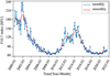Fig. 1 Annual variation of 10.7 cm solar radio flux (F10.7) index. The blue curve is the average of the F10.7 index one month; the curve is the smooth data of F10.7 index, the dots are the scattered values of the monthly F10.7 index.

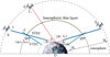Fig. 2 Supposing the TEC is compressed into an Ionospheric thin layer, the International Space Station (ISS)/Chinese Space Station (CSS) emitter to the receiver on Earth connections intersect at the Ionospheric thin layer, which point is called Ionospheric Pierce Point (IPP), VTEC is the TEC in the vertical direction at IPP and STEC is the slant TEC from ISS/CSS to the Earth. Hb and Ht are the heights from the Earth’s surface to the bottom and top spheres of the ionosphere layer of interest. The green arc between the left-side point IPP and the right-side one is visible from the ground station to the space station.

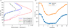Fig. 3 Variation of ionospheric electron density with altitude and diurnal variation of the ionosphere equivalent height (EH) for ISS/CSS and GNSS. (a) Variation of ionospheric electron density with altitude over the Observatoire de Paris (OP) for different times, which is calculated by the IRI-2016 model. (b) Diurnal variation of the ionosphere equivalent height (EH) for ISS/CSS and GNSS.

3 Ionospheric frequency shift effect on frequency transfer

In the ACES/CSS mission, the microwave frequencies and polarization directions are different, so we need different methods to process the ionospheric frequency shift. Namely, we use one-way frequency transfer, dual-frequency combination, and tri-frequency combination frequency transfer to eliminate various errors. The residual ionospheric frequency shift models accurate to different orders are formulated.

3.1 Ionospheric frequency shift in one-way frequency transfer

For one-way frequency transfer between two clocks, it is required to determine the photons frequency ratio f_A/f_B, where f_B is the proper frequency of the photon measured on the ground B and f_A is the proper frequency measured on satellite A (Blanchet et al. 2001; Linet & Teyssandier 2002; Shen et al. 2016, 2017), and the ratio can be expressed as: $$\frac{f_{\text{A}}}{f_{\text{B}}}=\frac{f_{\text{B}}+\text{Δ}{f}_{\text{B}}^{\text{dop}}+\text{Δ}{f}_{\text{B}}^{\text{rel}}+\text{Δ}{f}_{\text{B}}^{\text{ion}}+\text{Δ}{f}_{\text{B}}^{\text{tro}}+\text{Δ}{f}_{\text{B}}^{\text{ref}}+\text{Δ}{f}_{\text{B}}^{\text{tide}}}{f_{\text{B}}},$$(17)

where $\text{Δ}{f}_{\text{B}}^{\text{dop}}$ is the Doppler frequency shift, $\text{Δ}{f}_{\text{B}}^{\text{rel}}$ is the rela-tivistic frequency shift, $\text{Δ}{f}_{\text{B}}^{\text{tro}}$ is the tropospheric frequency shift, $\text{Δ}{f}_{\text{B}}^{\text{ion}}$ is the ionospheric frequency shift, $\text{Δ}{f}_{\text{B}}^{\text{ref}}$ is the bending effect on frequency and $\text{Δ}{f}_{\text{B}}^{\text{tide}}$ is the tide effect on frequency.

For one-way frequency transfer, we must construct a correction model for each error and estimate the correction parameters in Eq. (17). In this study, we only consider the ionospheric frequency shift $\text{Δ}{f}_{\text{B}}^{\text{ion}}/f_{\text{B}}$, Combining it with Eq. (9), the relative ionospheric frequency shift can be estimated as: $$\text{Δ}{f}_{\text{ion}}^1/f=40.3\frac{1}{c{f}^2}\frac{\text{ds}}{\text{d}t},$$(18) $$\text{Δ}{f}_{\text{ion}}^2/f=\mp \frac{7527}{2f^3}\overline{B_0\cos \theta }\frac{\text{d}s}{\text{d}t},$$(19) $$\text{Δ}{f}_{\text{ion}}^3/f=\frac{812.3}{c{f}^4}\eta N_{\text{m}}\frac{\text{d}s}{\text{d}t}.$$(20)

The coefficient in Eqs. (18)–(20) have the same meaning as those in Eq. (9), the superscripts 1, 2, and 3 represent the first-, second-, and third-order terms of the relative ionospheric frequency shifts, respectively.

3.2 Ionospheric frequency shift in dual-frequency combination method frequency transfer

In the CSS mission, a microwave signal with the frequency f_A emitted from the CSS antenna at point A and epoch t_A, and the ground station B emitted a microwave signal with the frequency f_B at the epoch t_B. At the epoch t′_B the ground station moved to B′ and received a f′_A signal and at the epoch t′_A the CSS antenna received a f′_B signal at the point A′, and these signals are recorded by their respective devices (see Fig. 4). Our study only considers the difference between emitting frequency and receiving frequency, the difference of T_AB or T′_AB ≤ 1µS (Meynadier et al. 2018), where T_AB = t_B – t_A and T′_AB = t′_B – t′_A can be ignored.

The CSS mission has two frequency signals with the same frequency of 30.4 GHz and different polarization directions. We can get the GRS by subtracting the two MWLs, which is called the dual-frequency combination method. In the dual-frequency combination method, we have one up-link f′_B/f_B and one downlink f′_A/f_A and the frequency ratio of emitting and receiving signals are expressed as: $${f^{\prime }}_{\text{A}}/f_{\text{A}}=\frac{f_{\text{A}}-\text{Δ}{f}_{\text{A}}^{\text{rel}}+\text{Δ}{f}_{\text{A}}^{ion}+\text{Δ}{f}_{\text{A}}^{\text{others}}}{f_{\text{A}}},$$(21) $${f^{\prime }}_{\text{B}}/f_{\text{B}}=\frac{f_{\text{B}}+\text{Δ}{f}_{\text{B}}^{\text{rel}}+\text{Δ}{f}_{\text{B}}^{\text{ion}}+\text{Δ}{f}_{\text{B}}^{\text{others}}}{f_{\text{B}}}.$$(22)

From Eq. (19), this pair of links have the same second-order ionospheric frequency shift but opposite in sign.

As T_AB ≤ 12 µs, the time of microwaves travel between spacecraft and ground station is about 1 ms (Meynadier et al. 2018). In such a short time, when the signals pass through the atmosphere, the effects of the troposphere and ionosphere are similar for up- and down-links, but the GRS equals in magnitude and opposite in sign. By subtracting Eq. (22) from Eq. (21), the GRS effects can be expressed as: $$\frac{\text{Δ}{f}_{\text{rel}}}{f_0}=\frac{1}{2}\left[\left(\frac{{f^{\prime }}_{\text{B}}}{f_{\text{B}}}-\frac{{f^{\prime }}_{\text{A}}}{f_{\text{A}}}\right)-\left(\frac{\text{Δ}{f}_{\text{B}}^{ion}}{f_{\text{B}}}-\frac{\text{Δ}{f}_{\text{A}}^{ion}}{f_{\text{A}}}\right)\right].$$(23)

Let I₁, I₂ and I₃ denote the coefficients of the first-, second-, and third-order terms, and then by combining Eqs. (18)–(20), the ionospheric frequency shift can be simplified as: $$\text{Δ}{f}_{\text{A}}^{\text{ion}}/f_{\text{A}}=\frac{I_1}{f_{\text{A}}^2}+\frac{I_2}{f_{\text{A}}^3}+\frac{I_3}{f_{\text{A}}^4},$$(24) $$\text{Δ}{f}_{\text{B}}^{\text{ion}}/f_{\text{B}}=\frac{I_1}{f_{\text{B}}^2}+\frac{I_2}{f_{\text{B}}^3}+\frac{I_3}{f_{\text{B}}^4}.$$(25)

For the up- and down-links, the cosθ or I₂ values have different signs. When we substitute Eqs. (24) and (25) with Eq. (23), the ionospheric frequency shifts are eliminated.

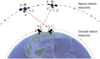Fig. 4 Dual-frequency transfer in the non-rotating frame for the CSS mission. In the CSS mission, fA = fB = 30.4 GHz, as the travel path is similar and the light speed, c, the signals reach the A′ and B′ at the time t′A and t′B, the difference of time is T′AB ≤ 1µs, with the atmosphere influencing the frequency in the same way.

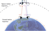Fig. 5 Tri-frequency transfer in the non-rotating frame for ACES mission. The ground station emitted a signal, f1, and the ISS antenna received f′1, immediately two down-link signals with frequencies of f2 and f3 emitted from the ISS antenna and received at the ground station with frequencies of f′2 and f′3. The emitted time is ti and the received time is t′i, i = 1, 2,3 (modified after Shen et al. 2016 and Sun et al. 2021).

3.3 Ionospheric frequency shift in tri-frequency combination method for frequency transfer

In the ACES mission, there are only three different frequency signals with one up-link f₁ and two down-links f₂ and f₃. The signals transfer is shown in Fig. 5: one up-link signal with a frequency, f₁, emitted from point B at the time, t₁, and received at point A at the time, t′₁, with the frequency f′₁, immediately two down-link signals with frequencies f₂ and f₃ emitted at point B′ at the time t₂ and t₃ (t₂ ≈ t₃), and received at point A′ at times of t′₂ and t′₃ (t′₂ ≈ t′₃) with frequencies of f′₂ and f′₃.

There are two different ways to test GRS: time comparison and frequency comparison. Meynadier et al. (2018) focused on time transfer and they used the code and carrier data to determine the time series of clock differences and then combined the two types of observations to calculate the ionospheric delay. The signals transfer of ACES is very similar to the GP-A experiment mission, so we considered choosing the tri-frequency combination method (Vessot & Levine 1979; Pound & Snider 1965; Shen et al. 2017) for the frequency transfer. In the GP-A experiment, the procedures are similar to the above description. The emitting signal frequency at the ground is f₀, after it arrives at the rocket and is transpondered to the ground, the received signal frequency at the ground is f″₀ (go-return link1 and link2); at the same time, the rocket emits a new signal with the frequency f₀ and the received signal’s frequency at the ground is denoted as f′₀ (one-way link3; Vessot & Levine 1979; Vessot et al. 1980). The tri-frequency combination model (Vessot & Levine 1979; Vessot et al. 1980; Shen et al. 2016, 2017; Kleppner et al. 1970) is expressed as: $$\text{Δ}f={f^{\prime }}_0-f_0-\frac{{f^{″}}_0-f_0}{2}.$$(26)

In the GP-A experiment setup, since the frequencies of all three microwave links are almost same, the frequency separation is required to prevent regeneration, which is realized by using rational multiples (P/Q = 76/49, N/M = 240/221, and R/S = 82/55) of the maser output frequency. By the frequency combination, the ionospheric frequency shift from f⁻¹ term was eliminated by choosing the uplink and downlink frequency according to the relationship $P/Q-\sqrt{2}\left(R/S\right){\left[1+{\left(N/M\right)}^2\right]}^{-1/2}=0$ (Vessot & Levine 1979; Vessot et al. 1980). Setting rational multiples into the equation, the ionospheric frequency shifts can be controlled to a magnitude smaller than 2 × 10⁻¹⁵, which satisfies the accuracy requirement of being lower than 5 × 10⁻¹⁵.

The frequency comparison has the following advantages: first, frequency comparisons need not consider phase ambiguity, which must be considered in time transfer. Second, frequency comparison may test GRS in a short time interval, while time comparison must accumulate data to solve the time-changing rate to test GRS. In the ACES/CSS mission, since the conditions are different, to eliminate the first-order ionospheric effect we use the modified tri-frequency model given by Sun et al. (2021) or Shen et al. (2021b). Sun et al. (2021) modified tri-frequency combination method for frequency transfer, and the one-way frequency transfer can be expressed as an equation (see Appendix A): $$\frac{{f^{\prime }}_1}{f_1}/\frac{{f^{\prime }}_2}{f_2}=\frac{m_1}{m_2}\times {\overline{A}}_{rel},$$(27)

where Ā_rel is the relativity effects which include the gravitational red-shift, transverse Doppler frequency shift and Shapiro effect, and m₁/m₂ expressed as (Sun et al. 2021): $$\frac{m_1}{m_2}=1+\left(\frac{f_2^2}{f_1^2}-1\right)\left(\frac{f_3^2}{f_3^2-f_2^2}\right)\left(\frac{{f^{\prime }}_2}{f_2}/\frac{{f^{\prime }}_3}{f_3}-1\right).$$(28)

The parameters in Eqs. (27) and (28) have the same notations as in Sun et al. (2021). This model can eliminate the first-order ionospheric frequency shift effect on the frequency transfer. Considering the higher order term ionospheric frequency shifts, Eq. (28) can be expressed as (for more details, see Appendix A): $$\begin{array}{l}\frac{m_1}{m_2}=1+\left(\frac{f_2^2}{f_1^2}-1\right)\left(\frac{f_3^2}{f_3^2-f_2^2}\right)\left(\frac{{f^{\prime }}_2}{f_2}/\frac{{f^{\prime }}_3}{f_3}-1\right)\hfill \\ +[\left(\pm \frac{f_2^3}{f_1^3}-1\right)-\left(\frac{f_2^2}{f_1^2}-1\right)\left(\frac{f_3^2}{f_3^2-f_2^2}\right)\hfill \\ \times \left(1-\frac{f_2^3}{f_3^3}\right)]\frac{7527}{2f_2^3}\overline{B_0\cos \theta }\frac{ds}{dt}\hfill \\ +[\left(\frac{f_2^4}{f_1^4}-1\right)-\left(\frac{f_2^2}{f_1^2}-1\right)\left(\frac{f_3^2}{f_3^2-f_2^2}\right)\hfill \\ \times \left(1-\frac{f_2^4}{f_3^4}\right)]\frac{812.3}{c{f}_2^4}\eta N_{\text{m}}\frac{ds}{dt},\hfill \end{array}$$(29)

where the term $\pm f_2^3/f_1^3$ takes the positive and negative signs for the left-hand and right-hand circularly polarized microwaves, respectively.

By combining Eqs. (27) and (29), we get the coefficients of the second- and third-order ionospheric frequency shifts, expressed as: $$C_2={\overline{A}}_{rel}\times \left[\left(\pm \frac{f_2^3}{f_1^3}-1\right)-\left(\frac{f_2^2}{f_1^2}-1\right)\left(\frac{f_3^2}{f_3^2-f_2^2}\right)\left(1-\frac{f_2^3}{f_3^3}\right)\right]$$(30) $$C_3={\overline{A}}_{rel}\times \left[\left(\frac{f_2^4}{f_1^4}-1\right)-\left(\frac{f_2^2}{f_1^2}-1\right)\left(\frac{f_3^2}{f_3^2-f_2^2}\right)\left(1-\frac{f_2^4}{f_3^4}\right)\right],$$(31)

f₁, f₂, and f₃ are the work frequencies. In the ACES, the coefficients of the second- and third-order ionospheric terms are about −3.5707 and −7.9252 for the frequencies of f₁ = 13.475 GHz, f₂ = 14.703 GHz, and f₃ = 2.248 GHz. If the model is used in the CSS mission, the coefficients of the second- and third-order ionospheric terms are about −0.0243 and −0.0534 for the frequencies of f₁ = 26.8 GHz, f₂ = 20.8 GHz, and f₃ = 30.4 GHz.

Fig. 6 Microwave transmission links of CSS (Chinese Space Station)/ACES (Atomic Clock Ensemble in Space). ACES mission has three links: one up-link and two down-links. CSS has four links: two up-links and two down-links.

4 Evaluation of the influence of high order ionospheric terms on frequency transfer

To study the ionospheric effects on frequency transmission, we must know the different frequency payloads by ACES and CSS. As shown in Fig. 6, there are one up-link and two down-links in the ACES. The Ku-band with the frequencies 13.475 GHz (up) and 14.703 GHz (down) and S-band with the frequency 2.248 GHz (down), respectively. In CSS, there are four frequencies, two up-links are K-band and Ka-band with the frequencies 26.8 GHz and 30.4 GHz, two down-links are K-band and Ka-band with the frequencies 20.8 GHz and 30.4 GHz. In addition, the polarization directions of the frequency payload by the CSS are different.

Table 1 shows the signals’ frequencies and their polarization directions. The CSS up-links polarization direction is left-hand circularly polarized. Down-links of CSS and all ACES links are right-hand circularly polarized. In the CSS, up-link2 and down-link2 have the same working frequency and different polarization directions. This setting will reduce the difficulty of data processing and make the data processing different from the ACES.

As the orbit altitude of both the CSS and the ISS is around 400 ~ 450 km, in this study, we chose the orbit data of the ISS when calculating the ionospheric frequency shifts of the CSS. The ISS orbit data can be downloaded from CELESTRAK².

Our experiment selected Observatoire de Paris (OP) as the ground station and the WGS84 ellipsoid as the reference ellipsoid. In Sect. 3.1, we established the model of ionospheric frequency shift, with the relevant parameters shown in Table 2.

4.1 Calculation of STEC rate and $\overline{B_0\text{\hspace{0.17em}cos\hspace{0.17em}\hspace{0.17em}}\theta }$

We calculated the STEC rate and ionospheric frequency shifts according to the method described in Sect. 2. First, we determined the orbits of ACES/ISS and the ground station coordinate. Second, we calculated the EH when the ISS/CSS is visible to the ground station each cycle. Then, we got the VTEC in the IPP and took it into the slant path of the spacecraft and the ground station by the mapping function. At last, we calculated the STEC rate of change by the difference between adjacent epochs.

We calculate the $\overline{B_0\text{\hspace{0.17em}cos\hspace{0.17em}\hspace{0.17em}}\theta }$ value via Eq. (16). Figure 7 shows that $\overline{B_0\text{\hspace{0.17em}cos\hspace{0.17em}\hspace{0.17em}}\theta }$ varies with the azimuth ranges from 0° to 360° and the elevation angles are 0°, 15°, 30°, 45°, 75°, 90°. Figures 7a,b show the values of $\overline{B_0\text{\hspace{0.17em}cos\hspace{0.17em}\hspace{0.17em}}\theta }$ for down-links, Figs. 7c,d give the values of $\overline{B_0\text{\hspace{0.17em}cos\hspace{0.17em}\hspace{0.17em}}\theta }$ for up-links. From Figs. 7a,c, we find that the value of $\overline{B_0\text{\hspace{0.17em}cos\hspace{0.17em}\hspace{0.17em}}\theta }$ is symmetric on 0° – 180° azimuth axis and increases gradually with the increase of elevation angle. Comparing Figs. 7b,d, we see that $\overline{B_0\text{\hspace{0.17em}cos\hspace{0.17em}\hspace{0.17em}}\theta }$ has the same value but the opposite sign for up and downlinks.

The absolute value of $\overline{B_0\text{\hspace{0.17em}cos\hspace{0.17em}\hspace{0.17em}}\theta }$ ranges from 0 to 5 × 10⁻⁵ T and changes significantly with the azimuth angle and elevation angle. We use the value of $\overline{B_0\text{\hspace{0.17em}cos\hspace{0.17em}\hspace{0.17em}}\theta }$ at the IPP with a one-second sampling interval to evaluate the second-order ionosphere frequency shift.

4.2 Ionospheric frequency shifts

We selected three frequencies of ACES mission and four frequencies of CSS (as shown in Table 1) to estimate the different orders of the ionospheric frequency shifts for one-way frequency transfer. Other relevant parameters in the experiment are shown in Table 2.

Here, we plot the absolute value distribution of different-order ionospheric frequency shifts in one orbital period by calculating the experiment data. Figure 8 shows the relative frequency shifts for ACES and CSS. The symbols f_ion1, f_ion2, and f_ion3 denote the absolute values of first-, second, and third-order frequency shifts calculated by Eqs. (18)–(20), respectively. We see that ionospheric frequency shifts become smaller with the space station closer to the ground station. Ionospheric frequency shifts decrease with the increase of the frequency. Figure 8a shows (for the ACES mission) the magnitude of the second-order ionospheric frequency shifts is about 10⁻¹⁵, and that of the third-order is approximately 10⁻¹⁷ for the frequency of 2.248 GHz. Figures 8b,c show (respectively) the second- and third-order ionospheric frequency shifts with magnitudes being 10⁻¹⁷ for frequencies 13.47 GHz and 14.7 GHz. Figures 8d–f show, for the CSS, that the magnitudes of the second-order ionospheric frequency shifts are about 10⁻¹⁸ for the three frequency signals and that of the third-order frequency shifts is smaller than 10⁻²⁰.

The accuracies of frequency transfer models for c⁻³ and c⁻⁴ are respectively about 5 × 10⁻¹⁷ (Blanchet et al. 2001) and 10⁻¹⁹ (Linet & Teyssandier 2002). When we consider the model accurate to c⁻³, the ionospheric frequency shifts bigger than 10⁻¹⁷ should be corrected. If the accuracy requirement is c⁻⁴, the ionospheric frequency shifts bigger than 10⁻¹⁹ should be corrected. According to characteristics of ACES and CSS missions, they will payload the atomic clocks with long-term stabilities of 3 × 10⁻¹⁶ (Cacciapuoti & Salomon 2011; Duchayne et al. 2009; Meynadier et al. 2018) and 8 × 10⁻¹⁸ (Wang 2021; Guo 2021). The third-order frequency shift is beyond the measurement accuracy of the atomic clocks, which can be ignored. In the ACES mission, the second-order terms of the S-band should be considered. The second-order ionospheric frequency shifts of the K-band and Ka-band must be eliminated or corrected for the CSS mission.

The CSS mission carried four microwave frequency signals, two of which have the same frequency and opposite polarization directions (see Table 1). We can use the dual-frequency combination method to make the frequency comparison and test the GRS to eliminate ionospheric frequency shifts (see Table 3). When we use the tri-frequency combination technique to transfer the frequency signals in ACES or CSS (as introduced in Sect. 3.3), we need to consider the effects of the second-order ionospheric frequency shift. We estimated the second-order ionospheric frequency shift coefficient value by Eq. (30), that is, −3.5707 for ACES and −0.0243 for CSS. By combining these coefficients with the values of frequency shifts with proper frequencies 14.703 GHz and 20.8 GHz (as shown in Table 3), the modified tri-frequency combination method data show that the second-order frequency shifts are about 9.280 × 10⁻¹⁷ for ACES and 2.231 × 10⁻¹⁹ for CSS.

In the same space environment, ionospheric frequency shift decreases with the increase of the frequency of microwave signals (see Table 3) and the CSS provides the higher frequency signals that can effectively reduce the impact of the ionosphere.

As the analysis given in Sect. 2.3, we know that electron density has a link to solar activity. It influences the TEC and ionospheric frequency shift. We plotted the second-order ionospheric frequency shifts of frequencies 2.248 GHz and 20.8 GHz in different solar activity years. Figure 9 shows the second-order ionospheric frequency shifts have similar distribution for the high solar activity year 2014 and low solar activity year 2021. In the lower left-hand corner of Figs. 9a,b, we enlarge the figure of 0 ~ 100 s, and the red dotted lines are 10⁻¹⁴ and 10⁻¹⁷ are for frequencies of 2.248 GHz and 20.8 GHz, respectively. It shows that the magnitudes of the ionospheric frequency shifts are about 10⁻¹⁴ in 2014 and 10⁻¹⁵ in 2021 for frequency 2.248 GHz, and 10⁻¹⁷ in 2014 and 10⁻¹⁸ in 2021 for frequency 20.8 GHz. The values of the ionospheric frequency shifts in 2014 are one order of magnitude bigger than in 2021.

Concerning the present atomic clock’s accuracy level and microwave frequencies for the ACES and the CSS missions, we need to consider the corrections of the second-order ionospheric frequency shifts, neglecting the third-order term. Although the tri-frequency combination may greatly reduce the ionospheric influences, the residual error of the second-order term could reach 10⁻¹⁶ during high solar activity years for ACES, thus it should be considered. In the future, the CSS mission may carry the OACs with long-term stability of 10⁻¹⁹. We note that we did not consider the third-order ionospheric frequency shift in this study. The second-order residual error with tri-frequency combination for the CSS is about 10⁻¹⁹, which ought to be corrected.

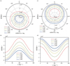Fig. 7 $\overline{B_0\text{\hspace{0.17em}cos\hspace{0.17em}\hspace{0.17em}}\theta }$ varies with the azimuth α and the elevation ɛ. (a) and (b) are the variations of the $\overline{B_0\text{\hspace{0.17em}cos\hspace{0.17em}\hspace{0.17em}}\theta }$ for the down-link, (c) and (d) are the variations of the $\overline{B_0\text{\hspace{0.17em}cos\hspace{0.17em}\hspace{0.17em}}\theta }$ for the up-link with azimuth for elevation angles 0°, 15°,30°, 45°, 75°, 90° at the OP.

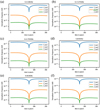Fig. 8 Ionospheric frequency shifts of one-way frequency transfer for ACES (a–c) and CSS (d–f). f_ion1, f_ion2, and f_ion3 denote the first-, second- and third-order frequency shifts of different frequency signals.

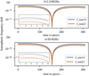Fig. 9 Absolute value of the ionospheric frequency shifts for second-order term $\text{Δ}{f}_{\text{ion}}^2/f$ for one-way frequency transfer. Here, f_ion14 and f_ion21 are the second-order ionospheric frequency shift in 2014 and 2021.

5 Conclusions

This study analyses ionosphere influence on frequency transfer and formulates higher order ionospheric frequency shift models for different frequency transfer methods. From the models, the second-order ionospheric frequency shift depends on the interaction of the ionosphere with the Earth’s magnetic field and TEC. These frequency shifts vary with the space station position and direction of the ray path.

In one-way frequency transfer, the second-order ionospheric frequency shifts reach 10⁻¹⁵ ~ 10⁻¹⁸ for different frequencies. The third-order ionospheric frequency shift is about 10⁻¹⁷ for a frequency of 2.248 GHz and smaller than 10⁻²⁰ for other frequencies. By analyzing the second-order ionospheric frequency shifts in years of high and low solar activity, we know it needs to be eliminated or corrected in the GRS test and frequency transfer in different periods.

According to the different designs of CSS and ACES, the frequency transfer between the space station and ground station is extracted by using the dual-frequency combination and tri-frequency combination methods. By analysis, we know the magnitude of the second-order ionospheric frequency shift by using the tri-frequency combination method is about 10⁻¹⁷ for ACES and 10⁻¹⁹ for CSS, corresponding to the magnitudes of influencing the accuracies of testing GRS with 1.0 × 10⁻⁶ and 1.0 × 10⁻⁸, respectively. If a higher accuracy level than 1.0 × 10⁻⁶ for ACES (or 1.0 × 10⁻⁸ for CSS) is needed, we can use the ionosphere model to correct the higher order ionospheric effects. Here we point out that the second-order ionospheric frequency shift is almost eliminated using the dual-frequency combination method for CSS frequency signal transfer.

There is a strong correlation between ionospheric frequency shift and TEC. In the years of high solar activity, the TEC could be one to two times greater than that in years of low solar activity. When the Sun experiences a magnetic storm, it is also possible for TEC to increase rapidly in a short time period. When its influence is comparable to the clock measurement accuracy, we need to correct the higher order ionospheric frequency shift.

Following on the development of time and frequency science and technology, especially OACs developments and the successful launch of the CSS, here we propose an approach that considers higher order ionospheric frequency contributions, which could achieve a higher order accuracy of testing GRS, based on a higher order term model of ionospheric frequency shift and different frequency transfer methods.

Acknowledgements

We appreciate two anonymous reviewer’s several-rounds comments and suggestions, which greatly improved the manuscript. This study is supported by the National Natural Science Foundations of China (NSFC) under Grants 42030105, 41721003, 42274011, Space Station Project (2020)228, and the Natural Science Foundation of Hubei Province of China under Grant 2019CFB611.

Appendix A Derivation of the modified tri-frequency combination formula

In the tri-frequency combination method for frequency transfer (Vessot & Levine 1979; Vessot et al. 1980; Shen et al. 2017; Sun et al. 2021), the propagation paths of the two down-link signals f′₂/f₂ and f′₃/f₃ are similar (see Fig. 5). Based on Equations 14–17 of Sun et al. (2021), dividing the f′₂/f₂ by f′₃/f₃, we obtain the expression: $$\begin{array}{l}\frac{f_2^{\prime }}{f_2}/\frac{f_3^{\prime }}{f_3}=1+\frac{\text{Δ}{f}_{2\left(ion\right)}}{f_2}-\frac{\text{Δ}{f}_{3\left(ion\right)}}{f_3}\hfill \\ +\left(1-\frac{f_2^2}{f_3^2}\right)\left[\delta f_{2\left(\text{refr}\right)}+\frac{40.3N_{\text{e}}{N}_{\text{AB}}\cdot v_{\text{A}}}{c{f}_2^2}\right],\hfill \end{array}$$(A.1)

where δf_2(refr) is the frequency shift caused by the refraction N_AB is the unit vector from point A to point B and v_A is the velocity vector at point A. From Equation 9, the two downlink signals’ ionospheric frequency shifts are: $$\text{Δ}{f}_{j\left(\text{ion}\right)}=\frac{40.3ds}{c{f}_j}\frac{ds}{dt}+\frac{7527}{2f_j^2}\overline{B_0\cos \theta }\frac{ds}{dt}+\frac{812.3}{c{f}_j^3}\eta N_{\text{m}}\frac{ds}{dt},j=2,3.$$(A.2)

Substituting Equation A.2 into Equation A.1, we obtain: $$\begin{array}{l}\frac{f_2^{\prime }}{f_2}/\frac{f_3^{\prime }}{f_3}=1+\left(\frac{40.3}{c{f}_2^2}\frac{ds}{dt}+\frac{7527}{2f_2^3}\overline{B_0\cos \theta }\frac{ds}{dt}+\frac{812.3}{c{f}_2^4}\eta N_{\text{m}}\frac{ds}{dt}\right)\hfill \\ -\left(\frac{40.3}{c{f}_3^2}\frac{ds}{dt}+\frac{7527}{2f_3^3}\overline{B_0\cos \theta }\frac{ds}{dt}+\frac{812.3}{c{f}_3^4}\eta N_{\text{m}}\frac{ds}{dt}\right)\hfill \\ +\left(1-\frac{f_2^2}{f_3^2}\right)\left[\delta f_{2\left(\text{refr}\right)}+\frac{40.3N_{\text{e}}{N}_{\text{AB}}\cdot v_{\text{A}}}{c{f}_2^2}\right].\hfill \end{array}$$(A.3)

By rearranging the relevant terms, Equation A.3 can be written as: $$\begin{array}{l}\frac{f_2^{\prime }}{f_2}/\frac{f_3^{\prime }}{f_3}=1+\left(1-\frac{f_2^3}{f_3^3}\right)\frac{7527}{2f_2^3}\overline{B_0\cos \theta }\frac{ds}{dt}+\left(1-\frac{f_2^4}{f_3^4}\right)\frac{812.3}{c{f}_2^4}\eta N_{\text{m}}\frac{ds}{dt}\hfill \\ +\left(1-\frac{f_2^2}{f_3^2}\right)\left[\frac{40.3}{c{f}_2^2}\frac{ds}{dt}+\delta f_{2\left(\text{refr}\right)}+\frac{40.3N_{\text{e}}{N}_{\text{AB}}\cdot v_{\text{A}}}{c{f}_2^2}\right].\hfill \end{array}$$(A.4)

Thus, we can define: $$\delta f_k=\left[\frac{40.3}{c{f}_k^2}\frac{ds}{dt}+\delta f_{k\left(\text{refr}\right)}+\frac{40.3N_{\text{e}}{N}_{\text{AB}}\cdot v_{\text{A}}}{c{f}_k^2}\right],k=1,2,$$(A.5)

from Sun et al. (2021)’s study, since δf_k(refr) is inversely proportional to the square of the frequency f_k, we get $\delta f_k=\kappa /f_k^2$, where κ is a constant, namely $\delta f_1{f}_1^2=\delta f_2{f}_2^2$. Hence, we have $$\delta f_2=\left(f_1^2/f_2^2\right)\delta f_1.$$(A.6)

Equation (A.4) can be written as: $$\begin{array}{l}\frac{f_2^{\prime }}{f_2}/\frac{f_3^{\prime }}{f_3}=1+\left(1-\frac{f_2^2}{f_3^2}\right)\delta f_2+\left(1-\frac{f_2^3}{f_3^3}\right)\frac{7527}{2f_2^3}\overline{{\text{B}}_0\cos \theta }\frac{ds}{dt}\hfill \\ +\left(1-\frac{f_2^4}{f_3^4}\right)\frac{812.3}{c{f}_2^4}\eta N_{\text{m}}\frac{ds}{dt}.\hfill \end{array}$$(A.7)

Similarly, for the up- and down-links, we know θ_u = 180° – θ_d and cosθ_u = –cosθ_d = –cosθ, the up- and down-links have the different sign, so: $$\begin{array}{l}\frac{f_1^{\prime }}{f_1}/\frac{f_2^{\prime }}{f_2}=[1+\left(1-\frac{f_1^2}{f_2^2}\right)\delta f_1+\left(\pm 1-\frac{f_1^3}{f_2^3}\right)\frac{7527}{2f_1^3}\overline{{\text{B}}_0\cos \theta }\frac{ds}{dt}\hfill \\ +\left(1-\frac{f_1^4}{f_2^4}\right)\frac{812.3}{c{f}_1^4}\eta N_{\text{m}}\frac{ds}{dt}]\times {\overline{A}}_{\text{rel}},\hfill \end{array}$$(A.8)

which includes the f₁ frequency shift δf₁, namely, $\frac{f_1^{\prime }}{f_1}/\frac{f_2^{\prime }}{f_2}$ is expressed by δf₁. We may also express $\frac{f_1^{\prime }}{f_1}/\frac{f_2^{\prime }}{f_2}$ by f₂ frequency shift δf₂ by following procedure. We multiply $\frac{f_2^2}{f_1^2}\frac{f_1^2}{f_2^2}$, $\frac{f_2^3}{f_1^3}\frac{f_1^3}{f_2^3}$, $\frac{f_2^4}{f_1^4}\frac{f_1^4}{f_2^4}$ (they are equal to 1) with the second, third, and fourth terms of square brackets in Equation A.8, respectively, obtaining the expression: $$\begin{array}{l}\frac{f_1^{\prime }}{f_1}/\frac{f_2^{\prime }}{f_2}=[1+\frac{f_2^2}{f_1^2}\frac{f_1^2}{f_2^2}\left(1-\frac{f_1^2}{f_2^2}\right)\delta f_1+\frac{f_2^3}{f_1^3}\frac{f_1^3}{f_2^3}\left(\pm 1-\frac{f_1^3}{f_2^3}\right)\hfill \\ \times \frac{7527}{2f_1^3}\overline{B_0\cos \theta }\frac{ds}{dt}+\frac{f_2^4}{f_1^4}\frac{f_1^4}{f_2^4}\left(1-\frac{f_1^4}{f_2^4}\right)\frac{812.3}{c{f}_1^4}\eta N_{\text{m}}\frac{ds}{dt}]\times {\overline{A}}_{\text{rel}},\hfill \end{array}$$(A.9)

and after rearranging, we get $$\begin{array}{l}\frac{f_1^{\prime }}{f_1}/\frac{f_2^{\prime }}{f_2}=[1+\left(\frac{f_2^2}{f_1^2}-1\right)\frac{f_1^2}{f_2^2}\delta f_1+\left(\pm \frac{f_2^3}{f_1^3}-1\right)\frac{7527}{2f_2^3}\overline{B_0\cos \theta }\frac{ds}{dt}\hfill \\ +\left(\frac{f_2^4}{f_1^4}-1\right)\frac{812.3}{c{f}_2^4}\eta N_{\text{m}}\frac{ds}{dt}]\times {\overline{A}}_{\text{rel}}.\hfill \end{array}$$(A.10)

Substituting Equation A.6 in Equation A.10, we get $$\begin{array}{l}\frac{f_1^{\prime }}{f_1}/\frac{f_2^{\prime }}{f_2}=[1+\left(\frac{f_2^2}{f_1^2}-1\right)\delta f_2+\left(\pm \frac{f_2^3}{f_1^3}-1\right)\frac{7527}{2f_2^3}\overline{B_0\cos \theta }\frac{ds}{dt}\hfill \\ +\left(\frac{f_2^4}{f_1^4}-1\right)\frac{812.3}{c{f}_2^4}\eta N_{\text{m}}\frac{ds}{dt}]\times {\overline{A}}_{\text{rel}},\hfill \end{array}$$(A.11)

where δf₂ can be obtained from Equation A.7: $$\begin{array}{l}\delta f_2=\left(\frac{f_3^2}{f_3^2-f_2^2}\right)[\frac{f_2^{\prime }}{f_2}/\frac{f_3^{\prime }}{f_3}-1-\left(1-\frac{f_2^3}{f_3^3}\right)\frac{7527}{2f_2^3}\overline{B_0\cos \theta }\frac{ds}{dt}\hfill \\ -\left(1-\frac{f_2^4}{f_3^4}\right)\frac{812.3}{c{f}_2^4}\eta N_{\text{m}}\frac{ds}{dt}].\hfill \end{array}$$(A.12)

Substituting Equation A.12 into Equation A.11, we obtain Equation 29, namely: $$\begin{array}{l}\frac{m_1}{m_2}=1+\left(\frac{f_2^2}{f_1^2}-1\right)\left(\frac{f_3^2}{f_3^2-f_2^2}\right)\left(\frac{f_2^{\prime }}{f_2}/\frac{f_3^{\prime }}{f_3}-1\right)\hfill \\ +[\left(\pm \frac{f_2^3}{f_1^3}-1\right)-\left(\frac{f_2^2}{f_1^2}-1\right)\left(\frac{f_3^2}{f_3^2-f_2^2}\right)\hfill \\ \times \left(1-\frac{f_2^3}{f_3^3}\right)]\frac{7527}{2f_2^3}\overline{B_0\cos \theta }\frac{ds}{dt}\hfill \\ +[\left(\frac{f_2^4}{f_1^4}-1\right)-\left(\frac{f_2^2}{f_1^2}-1\right)\left(\frac{f_3^2}{f_3^2-f_2^2}\right)\hfill \\ \times \left(1-\frac{f_2^4}{f_3^4}\right)]\frac{812.3}{c{f}_2^4}\eta N_{\text{m}}\frac{ds}{dt}.\hfill \end{array}$$(A.13)

From Equations A.8, A.11, and A.13, we can estimate the magnitude of the higher order ionospheric frequency shifts.

References

All Tables

All Figures

	Fig. 1 Annual variation of 10.7 cm solar radio flux (F10.7) index. The blue curve is the average of the F10.7 index one month; the curve is the smooth data of F10.7 index, the dots are the scattered values of the monthly F10.7 index.
In the text

Fig. 2 Supposing the TEC is compressed into an Ionospheric thin layer, the International Space Station (ISS)/Chinese Space Station (CSS) emitter to the receiver on Earth connections intersect at the Ionospheric thin layer, which point is called Ionospheric Pierce Point (IPP), VTEC is the TEC in the vertical direction at IPP and STEC is the slant TEC from ISS/CSS to the Earth. Hb and Ht are the heights from the Earth’s surface to the bottom and top spheres of the ionosphere layer of interest. The green arc between the left-side point IPP and the right-side one is visible from the ground station to the space station.

In the text

	Fig. 3 Variation of ionospheric electron density with altitude and diurnal variation of the ionosphere equivalent height (EH) for ISS/CSS and GNSS. (a) Variation of ionospheric electron density with altitude over the Observatoire de Paris (OP) for different times, which is calculated by the IRI-2016 model. (b) Diurnal variation of the ionosphere equivalent height (EH) for ISS/CSS and GNSS.
In the text

	Fig. 4 Dual-frequency transfer in the non-rotating frame for the CSS mission. In the CSS mission, fA = fB = 30.4 GHz, as the travel path is similar and the light speed, c, the signals reach the A′ and B′ at the time t′A and t′B, the difference of time is T′AB ≤ 1µs, with the atmosphere influencing the frequency in the same way.
In the text

Fig. 5 Tri-frequency transfer in the non-rotating frame for ACES mission. The ground station emitted a signal, f1, and the ISS antenna received f′1, immediately two down-link signals with frequencies of f2 and f3 emitted from the ISS antenna and received at the ground station with frequencies of f′2 and f′3. The emitted time is ti and the received time is t′i, i = 1, 2,3 (modified after Shen et al. 2016 and Sun et al. 2021).

In the text

	Fig. 6 Microwave transmission links of CSS (Chinese Space Station)/ACES (Atomic Clock Ensemble in Space). ACES mission has three links: one up-link and two down-links. CSS has four links: two up-links and two down-links.
In the text

Fig. 7 $\overline{B_0\text{\hspace{0.17em}cos\hspace{0.17em}\hspace{0.17em}}\theta }$ varies with the azimuth α and the elevation ɛ. (a) and (b) are the variations of the $\overline{B_0\text{\hspace{0.17em}cos\hspace{0.17em}\hspace{0.17em}}\theta }$ for the down-link, (c) and (d) are the variations of the $\overline{B_0\text{\hspace{0.17em}cos\hspace{0.17em}\hspace{0.17em}}\theta }$ for the up-link with azimuth for elevation angles 0°, 15°,30°, 45°, 75°, 90° at the OP.

In the text

	Fig. 8 Ionospheric frequency shifts of one-way frequency transfer for ACES (a–c) and CSS (d–f). f_ion1, f_ion2, and f_ion3 denote the first-, second- and third-order frequency shifts of different frequency signals.
In the text

	Fig. 9 Absolute value of the ionospheric frequency shifts for second-order term $\text{Δ}{f}_{\text{ion}}^2/f$ for one-way frequency transfer. Here, f_ion14 and f_ion21 are the second-order ionospheric frequency shift in 2014 and 2021.
In the text

References

- Alizadeh, M. M., Wijaya, D. D., Hobiger, T., Weber, R., & Schuh, H. 2013, in Atmospheric Effects in Space Geodesy (Springer), 35 [CrossRef] [Google Scholar]
- Alken, P., Thebault, E., Beggan, C., et al. 2021, Earth Planets Space, 73, 1 [CrossRef] [Google Scholar]
- Angrisano, A., Gaglione, S., Gioia, C., Massaro, M., & Robustelli, U. 2013, Acta Geophysica, 61, 1457 [NASA ADS] [CrossRef] [Google Scholar]
- Appleton, E. V. 1932, Inst. Electr. Eng. Proc. Wireless Sect. Inst., 7, 257 [Google Scholar]
- Bassiri, S., & Hajj, G. A. 1993, Manuscripta Geodaetica, 18, 280 [Google Scholar]
- Bennett, J. 1968, Aust. J. Phys., 21, 259 [NASA ADS] [CrossRef] [Google Scholar]
- Bilitza, D., Altadill, D., Truhlik, V., et al. 2017, Space Weather, 15, 418 [CrossRef] [Google Scholar]
- Blanchet, L., Salomon, C., Teyssandier, P., & Wolf, P. 2001, A&A, 370, 320 [NASA ADS] [CrossRef] [EDP Sciences] [Google Scholar]
- Brunner, F. K., & Gu, M. 1991, Manuscripta Geodaetica, 16, 205 [Google Scholar]
- Cacciapuoti, L., & Salomon, C. 2011, in J. Phys. Conf. Ser., 327, 012049 [NASA ADS] [CrossRef] [Google Scholar]
- Cai, C., Shen, W. B., Shen, Z., & Xu, W. 2020, IEEE Access, 8, 204283 [NASA ADS] [CrossRef] [Google Scholar]
- Davies, K. 1965, Ionospheric Radio Propagation, 80 (US Department of Commerce, National Bureau of Standards) [Google Scholar]
- Delva, P., Lodewyck, J., Bilicki, S., et al. 2017, Phys. Rev. Lett., 118, 221102 [NASA ADS] [CrossRef] [Google Scholar]
- Duchayne, L. 2008, PhD thesis, Observatoire de Paris, France [Google Scholar]
- Duchayne, L., Mercier, F., & Wolf, P. 2009, A&A, 504, 653 [NASA ADS] [CrossRef] [EDP Sciences] [Google Scholar]
- Einstein, A. 1915, in Sitzungsberichte der Koniglich Preußischen Akademie der Wissenschaften, 844 [Google Scholar]
- Guo, Y. 2021, in The 12th China Satellite Navigation Conference, CSNC 2021 [Google Scholar]
- Hartmann, G., & Leitinger, R. 1984, Bull. Géodésique, 58, 109 [Google Scholar]
- Hoque, M. M., & Jakowski, N. 2007, J. Geodesy, 81, 259 [NASA ADS] [CrossRef] [Google Scholar]
- Hoque, M. M., & Jakowski, N. 2008a, Radio Sci., 43, 1 [NASA ADS] [CrossRef] [Google Scholar]
- Hoque, M. M., & Jakowski, N. 2008b, GPS Solutions, 12, 87 [CrossRef] [Google Scholar]
- Hoque, M. M., & Jakowski, N. 2010, Adv. Space Res., 46, 162 [NASA ADS] [CrossRef] [Google Scholar]
- Hoque, M. M., & Jakowski, N. 2012, Global Navigation Satellite Systems: Signal, Theory and Applications [Google Scholar]
- Hoque, M. M., & Jakowski, N. 2015, J. Geodesy, 89, 391 [NASA ADS] [CrossRef] [Google Scholar]
- Jacobs, J. A., & Watanabe, T. 1966, Radio Sci., 1, 257 [NASA ADS] [CrossRef] [Google Scholar]
- Jakowski, N., Sardon, E., & Schlueter, S. 1998, Adv. Space Res., 22, 803 [NASA ADS] [CrossRef] [Google Scholar]
- Kleppner, D., Vessot, R. F. C., & Ramsey, N. F. 1970, Astrophys. Space Sci., 6, 13 [NASA ADS] [CrossRef] [Google Scholar]
- Klobuchar, J. A. 1987, IEEE Trans. Aerospace Electron. Syst., 325 [CrossRef] [Google Scholar]
- Kopeikin, S. M., Mazurova, E. M., & Karpik, A. P. 2015, Phys. Lett. A, 379, 1555 [NASA ADS] [CrossRef] [Google Scholar]
- Linet, B., & Teyssandier, P. 2002, Phys. Rev. D, 66, 024045 [Google Scholar]
- Liu, A., Wang, N., Li, Z., Wang, Z., & Yuan, H. 2019, Adv. Space Res., 63, 3978 [NASA ADS] [CrossRef] [Google Scholar]
- Liu, C., Liu, C., Bao, Y., & Feng, X. 2018a, Chinese J. Space Sci., 038, 37 [NASA ADS] [CrossRef] [Google Scholar]
- Liu, T., Zhang, B., Yuan, Y., & Li, M. 2018b, J. Geodesy, 92, 1 [Google Scholar]
- McGrew, W. F., Zhang, X., Fasano, R. J., et al. 2018, Nature, 564, 87 [NASA ADS] [CrossRef] [Google Scholar]
- Meynadier, F., Delva, P., le Poncin-Lafitte, C., Guerlin, C., & Wolf, P. 2018, Class. Quant. Grav., 35, 035018 [NASA ADS] [CrossRef] [Google Scholar]
- Nakamura, T., Davila-Rodriguez, J., Leopardi, H., et al. 2020, Science, 368, 889 [NASA ADS] [CrossRef] [Google Scholar]
- Namazov, S., Novikov, V., & Khmel’Nitskii, I. 1975, Radiophys. Quant. Electron., 18, 345 [NASA ADS] [CrossRef] [Google Scholar]
- Odijk, D. 2002, Publ. Geodesy, 52 [Google Scholar]
- Oelker, E., Hutson, R., Kennedy, C., et al. 2019, Nat. Photon., 13, 714 [NASA ADS] [CrossRef] [Google Scholar]
- Pound, R. V., & Snider, J. L. 1965, Phys. Rev., 140, B788 [NASA ADS] [CrossRef] [Google Scholar]
- Riehle, F. 2015, Comptes Rendus Physique, 16, 506 [CrossRef] [Google Scholar]
- Shen, W. B., Chao, D., & Jin, B. 1993, Boll. Geod. Sci. Affni., 52, 207 [Google Scholar]
- Shen, Z., Shen, W. B., & Zhang, S. 2016, Geophys. J. Int., 206, 1162 [NASA ADS] [CrossRef] [Google Scholar]
- Shen, Z., Shen, W. B., & Zhang, S. 2017, Surv. Geophys., 38, 757 [NASA ADS] [CrossRef] [Google Scholar]
- Shen, Q., Guan, J. Y., Zeng, T., et al. 2021a, Optica, 8, 471 [NASA ADS] [CrossRef] [Google Scholar]
- Shen, Z., Shen, W. B., Zhang, T., et al. 2021b, Adv. Space Res., 68, 2776 [NASA ADS] [CrossRef] [Google Scholar]
- Snider, J. L. 1972, Phys. Rev. Lett., 28, 853 [NASA ADS] [CrossRef] [Google Scholar]
- Sun, X., Shen, W. B., Shen, Z., et al. 2021, Eur. Phys. J. C, 81, 1 [NASA ADS] [CrossRef] [Google Scholar]
- Tariku, Y. A. 2020, AJ, 160, 185 [NASA ADS] [CrossRef] [Google Scholar]
- Vessot, R. F. C., & Levine, M. 1979, Gen. Relativity and Gravitation, 10, 181 [NASA ADS] [CrossRef] [Google Scholar]
- Vessot, R. F. C., Levine, M. W., Mattison, E. M., et al. 1980, Phys. Rev. Lett., 45, 2081 [NASA ADS] [CrossRef] [Google Scholar]
- Wang, W. 2021, in The 12th China Satellite Navigation Conference, CSNC 2021 [Google Scholar]
- Weinberg, S. 1972, Gravitation and Cosmology: Principles and Applications of the General Theory of Relativity (Wiley) [Google Scholar]
- Wolfson, R. 2009, Essential University (Physics Volume 2), 2 (Pearson Education India) [Google Scholar]
All Tables
Atomic Clock Ensemble in Space (ACES) and Chinese Space Station (CSS) frequencies and their polarization direction.