| Issue |
A&A
Volume 677, September 2023
|
|
|---|---|---|
| Article Number | A20 | |
| Number of page(s) | 14 | |
| Section | Stellar structure and evolution | |
| DOI | https://doi.org/10.1051/0004-6361/202346703 | |
| Published online | 24 August 2023 | |
Environmental dependence of Type IIn supernova properties
1
National Astronomical Observatory of Japan, National Institutes of Natural Sciences, 2-21-1 Osawa, Mitaka, Tokyo 181-8588, Japan
e-mail: takashi.moriya@nao.ac.jp
2
School of Physics and Astronomy, Faculty of Science, Monash University, Clayton, Victoria 3800, Australia
3
Institute of Space Sciences (ICE, CSIC), Campus UAB, Carrer de Can Magrans, s/n, 08193 Barcelona, Spain
e-mail: lgalbany@ice.csic.es
4
Institut d’Estudis Espacials de Catalunya (IEEC), 08034 Barcelona, Spain
5
European Southern Observatory, Alonso de Córdova 3107, Casilla 19, Santiago, Chile
6
Millennium Institute of Astrophysics MAS, Nuncio Monsenor Sotero Sanz 100, Off. 104, Providencia, Santiago, Chile
7
Tuorla Observatory, Department of Physics and Astronomy, University of Turku, 20014 Turku, Finland
8
Finnish Centre for Astronomy with ESO (FINCA), University of Turku, 20014 Turku, Finland
9
Instituto de Astronomía, Universidad Nacional Autónoma de México, A.P. 70-264, 04510 Mexico DF, Mexico
10
Department of Physics, University of Warwick, Coventry CV4 7AL, UK
11
Núcleo de Astronomía de la Facultad de Ingeniería y Ciencias, Universidad Diego Portales, Av. Ej ército 441, Santiago, Chile
12
Department of Astronomy, The Ohio State University, 140 W. 18th Ave., Columbus, OH 43210, USA
13
Center for Cosmology and Astroparticle Physics (CCAPP), The Ohio State University, 191 W. Woodruff Ave., Columbus, OH 43210, USA
14
Kavli Institute for Astronomy and Astrophysics, Peking University, Yi He Yuan Road 5, Hai Dian District, Beijing 100871, PR China
15
Department of Particle Physics and Astrophysics, Weizmann Institute of Science, 234 Herzl St, 7610001 Rehovot, Israel
Received:
19
April
2023
Accepted:
15
June
2023
Type IIn supernovae occur when stellar explosions are surrounded by dense hydrogen-rich circumstellar matter. The dense circumstellar matter is likely formed by extreme mass loss from their progenitors shortly before they explode. The nature of Type IIn supernova progenitors and the mass-loss mechanism forming the dense circumstellar matter are still unknown. In this work, we investigate whether Type IIn supernova properties and their local environments are correlated. We use Type IIn supernovae with well-observed light curves and host-galaxy integral field spectroscopic data so that we can estimate both supernova and environmental properties. We find that Type IIn supernovae with a higher peak luminosity tend to occur in environments with lower metallicity and/or younger stellar populations. The circumstellar matter density around Type IIn supernovae is not significantly correlated with metallicity, so the mass-loss mechanism forming the dense circumstellar matter around Type IIn supernovae might be insensitive to metallicity.
Key words: supernovae: general / stars: massive / stars: mass-loss
© The Authors 2023
 Open Access article, published by EDP Sciences, under the terms of the Creative Commons Attribution License (https://creativecommons.org/licenses/by/4.0), which permits unrestricted use, distribution, and reproduction in any medium, provided the original work is properly cited.
This article is published in open access under the Subscribe to Open model. Subscribe to A&A to support open access publication.
1. Introduction
Type IIn supernovae (SNe IIn) occur when stars explode within a dense hydrogen-rich circumstellar matter (CSM; Schlegel 1990; Filippenko 1997). The dense CSM is created by strong mass loss from the progenitors with typical mass-loss rate estimates of more than 10−4 M⊙ yr−1 (e.g., Kiewe et al. 2012; Taddia et al. 2013; Moriya et al. 2014; Ofek et al. 2014a). These mass-loss rates are much higher than those measured for typical stars (e.g., Smith 2014), and the progenitors and mass-loss mechanisms of SNe IIn are still not well understood. It is suggested that the high mass-loss rates are similar to those of massive (≳25 M⊙) luminous blue variable stars (LBVs; e.g., Weis & Bomans 2020). The progenitor of the Type IIn SN 2005gl is indeed consistent with a massive LBV (Gal-Yam & Leonard 2009). On the other hand, the progenitor of the Type IIn SN 2008S had a relatively low mass (≃10 M⊙; Prieto et al. 2008). These two SN IIn progenitors suggest that the progenitors and mass-loss mechanisms of SNe IIn are diverse. In addition, SNe Ia are sometimes hidden below dense hydrogen-rich CSM and are observed as SNe IIn (SN Ia-CSM; e.g., Sharma et al. 2023).
The local environments in which SNe explode provide rich information about their progenitors (e.g., Pessi et al. 2023a,b; see Anderson et al. 2015 for a review). For example, SNe II and Ibc but not SNe Ia preferentially occur in star-forming environments, which indicates that SNe II and Ibc are associated with massive star explosions (e.g., Li et al. 2011; Galbany et al. 2014). There have been several studies of the local environments of SNe IIn. Habergham et al. (2014) found that their locations are not necessarily associated with the most actively star-forming regions in their host galaxies, and some may not be associated with very massive progenitors. A later study by Ransome et al. (2022) found that 60% of SNe IIn originate from actively star-forming regions and could be linked to very massive progenitors, such as LBVs. The remaining 40% were not correlated with ongoing star formation and could have relatively low-mass progenitors (see also Kuncarayakti et al. 2018). Similarly, Galbany et al. (2018) estimated the age distributions of SN IIn progenitors based on spectra of their surroundings and found that they may have a bimodal age distribution with one peak at 0 − 20 Myr and the other at 100 − 300 Myr. These studies suggest that SN IIn progenitors are a mixture of massive (≳25 M⊙, like LBVs) and low-mass stars (≃10 M⊙, like the progenitor of SN 2008S). Other local properties may also provide information about their nature. For example, Taddia et al. (2015) investigated the relation between the SN IIn progenitor mass-loss rates and their local metallicity. They found that the progenitors of SNe IIn may have higher mass-loss rates in higher-metallicity environments.
In this work, we explore the environmental dependence of the SN IIn properties by using SNe IIn with integral-field spectroscopy (IFS) of their host galaxies. The IFS data allow us to estimate not only the metallicity, but also environmental parameters, such as the local star formation rates (SFRs). We introduce our SN IIn samples in Sect. 2. We estimate the local environmental parameters of the SN IIn explosion sites in Sect. 3 and estimate the SN IIn properties in Sect. 4. We investigate possible correlations between the environmental and SN properties in Sect. 5 and discuss them in Sect. 6. We conclude this paper in Sect. 7. We adopt a ΛCDM cosmology with H0 = 68.3 km s−1 Mpc−1, ΩM = 0.28, and ΩΛ = 0.72 (Hinshaw et al. 2013).
2. Sample definition
We constructed our sample using all galaxies observed with IFS from the PISCO, AMUSING, and MaNGA surveys to host a Type IIn SN. The PMAS/PPak Integral field Supernova hosts COmpilation (PISCO; Galbany et al. 2018) is a compilation of IFS observations of more than 400 SN host galaxies obtained with the Potsdam Multi Aperture Spectograph (PMAS; Roth et al. 2005) on the 3.5 m telescope of the Centro Astronomico Hispano-Aleman (CAHA) at the Calar Alto Observatory. The observations were obtained in PPak mode (Verheijen et al. 2004; Kelz et al. 2006). About one-third of the objects were observed by the CALIFA survey (Sánchez et al. 2016). Each observation consists of a 3D datacube with a 100% covering factor within a hexagonal field of view (FoV) of ∼1.3 arcmin2, with 1″ × 1″ spatial pixels (spaxels) and a spectral resolution of ∼6 Å over the wavelength range 3750−7300 Å, providing ∼4000 spectra per object.
The All-weather MUse Supernova Integral-field of Nearby Galaxies (AMUSING; Galbany et al. 2016a; López-Cobá et al. 2020; Galbany et al., in prep.) survey has been running for 11 semesters (P95–P106) and has compiled observations for more than 800 nearby SN host galaxies with the Multi-Unit Spectroscopic Explorer (MUSE; Bacon et al. 2014), located at the Nasmyth B focus of Yepun, the VLT UT4 telescope at Cerro Paranal Observatory. MUSE is composed of 24 identical IFS. Wide-field mode (WFM) samples a nearly contiguous 1 arcmin2 FoV with spaxels of 0.2 × 0.2 arcsec, and over a wavelength range of 4650−9300 Å with a mean resolution of R ∼ 3000. Each 3D cube consists of ∼100 000 spectra per pointing.
The Mapping Nearby Galaxies at APO (MaNGA; Bundy et al. 2015) was part of Sloan Digital Sky Survey (SDSS) IV (Blanton et al. 2017) and obtained IFS data of ∼10 000 nearby galaxies using 17 units of different hexagonal FoVs ranging from 12 to 32 arcsec in diameter at the 2.5 m SDSS telescope at the Apache Point Observatory in New Mexico. The square spaxels are 0.5 arcsec across, with a spectral resolution of R ∼ 2000 over a wavelength range of 3600−10 000 Å.
After a thorough search of these three datasets, we compiled an initial sample of 66 SN IIn host galaxies where the SN location was within the FoV. Next, we performed a thorough search for public light curves of the 66 SNe IIn in the literature. For objects that exploded in 2016 or after, we also used the ATLAS forced photometry service1 to obtain light curves (Tonry et al. 2018; Smith et al. 2020). For objects that exploded in 2018 or later, we used the ZTF forced photometry service (Masci et al. 2019). Only 17 of the 24 SNe IIn with publicly available data had light curves with a high enough quality and sampling during the rise for us to reliably determine the peak magnitude and rise time from explosion (see Sect. 4). In addition, we obtained light curves with good sampling from the All-Sky Automated Survey for SuperNovae (ASAS-SN; Shappee et al. 2014; Kochanek et al. 2017) and follow-up observations with the Las Cumbres Observatory Global Telescope network (LCOGT) for 4 additional SNe IIn (ASASSN-15ab, ASASSN-16bw, ASASSN-16in, and ASASSN-16jt). The LCOGT photometry was performed according to the procedures described in Chen et al. (2022). The final 21 SNe IIn in our sample are listed in Table 1.
SN IIn sample and its properties.
3. Local environments
The final sample of 21 SNe IIn is composed of 13 host galaxies observed with MUSE, 5 with PMAS, and 3 with MaNGA. The synthetic r-band images created from the IFS cubes are displayed in Fig. A.1.
We followed a similar procedure for all three IFS instruments. We extracted a rest-frame 2.7 arcsec diameter aperture spectrum for each SN position, corresponding to the worst spatial resolution in all the cubes. We analyzed the spectra as in Galbany et al. (2014, 2016b). We fit single stellar population (SSP) synthesis models to remove the underlying stellar continuum from the ionized gas-phase emission using STARLIGHT (Cid Fernandes et al. 2005, 2009). STARLIGHT determines the fractional contribution of different SSP models to the spectrum, accounting for dust extinction as a foreground screen. We used three parameters from the SSP fit: the stellar mass (M*), the average light-weighted stellar population age (t*, L), and the extinction derived from the stellar component (AV*).
The best-fit continuum model was then subtracted from each observed spectrum to leave the ionized gas-phase emission. Figure A.2 shows the aperture spectra, the best SSP fits, and their resulting gas-phase emission line spectra for all 21 SN IIn environments. We fit the emission lines needed to estimate oxygen abundances using several different methods. This included fitting Gaussian profiles to the Balmer Hαλ6563 and Hβλ4861 lines and the [O III] λ5007, [N II] λ6583, [S II] λλ6716,31 lines. The Hα and [N II] lines were fit simultaneously with [N II] λ6548 as three Gaussian profiles with fixed positions and similar width, but free amplitudes. In seven cases of relatively recent SNe (SN 2016bdu, SN 2016iaf, ASASSN-16bw, ASASSN-16in, ASASSN-16jt, SN 2017ghw, SN 2017hcc; see Fig. A.2), it was necessary to include a fourth component to account for a broad underlying Hα emission coming from the CSM interaction (see also Martínez-Rodríguez, in prep.).
The flux of the emission lines was corrected for dust extinction along the line of sight using the color excess (E(B − V)) estimate from the Hα/Hβ Balmer line flux ratios assuming the Case B recombination intrinsic ratio I(Hα)/I(Hβ) = 2.86 for T = 10 000 K, an electron density of 102 cm−3 (Osterbrock & Ferland 2006), and a Fitzpatrick (1999) extinction law.
The ongoing SFR can be directly estimated from the extinction-corrected Hα flux following Kennicutt (1998),
![$$ \begin{aligned} \mathrm{SFR} [M_\odot \,\mathrm{yr}^{-1}] = 7.9 \times 10^{-42}\,L(\mathrm{H}\alpha ), \end{aligned} $$](/articles/aa/full_html/2023/09/aa46703-23/aa46703-23-eq1.gif)
where
is the extinction-corrected Hα luminosity in units of erg s−1 and dL is the luminosity distance to the galaxy. The SFR density (ΣSFR) is obtained by dividing the SFR by the area of the aperture in kpc2, and the specific SFR (sSFR) is obtained by dividing the SFR by the stellar mass obtained from the STARLIGHT fit.
While the Hα flux is an indicator of the ongoing SFR, the Hα equivalent width, EW(Hα), is a measurement of how strong the emission line is compared with the stellar continuum. The stellar continuum is dominated by the contribution from old stars, which also contain most of the stellar mass. The EW(Hα) represents the fraction of young stars, and it can be thought of as an indicator of the strength of the ongoing SFR compared with the past SFR. It decreases with time when no ongoing star-formation is present. It is a reliable proxy for the age of the youngest stellar components (Sánchez et al. 2015; Kuncarayakti et al. 2016). To estimate EW(Hα), we divided the observed spectrum by the STARLIGHT fit and repeated the weighted nonlinear least-squares fit of the Hα line in the normalized spectra.
The most commonly used metallicity indicator in interstellar medium (ISM) studies is the oxygen abundance because it is the most abundant metal in the gas phase and has very strong optical nebular lines. We estimated the oxygen abundances, 12 + log(O/H), using three different empirical calibrations based on emission-line ratios. In particular, we used the N2 index with the Marino et al. (2013) calibrations updated from Pettini & Pagel (2004) based on the [N II]/Hα ratio,
![$$ \begin{aligned} 12 + \log \mathrm{(O/H)}_{\mathrm{N2}} = 8.743 + 0.462 \times \log \frac{[{{\text{N}}{\small { {\text{ II}}}}}]}{\mathrm{H}\alpha }, \end{aligned} $$](/articles/aa/full_html/2023/09/aa46703-23/aa46703-23-eq3.gif)
and the O3N2 index based on the difference between the logs of the [O III]/Hβ and [N II]/Hα ratios,
![$$ \begin{aligned} 12 + \log \mathrm{(O/H)}_{\mathrm{O3N2}} = 8.533 - 0.214 \times \log \left(\frac{[{{\text{O}}{\small { {\text{ III}}}}}]}{\mathrm{H}\beta }\frac{\mathrm{H}\alpha }{[{{\text{N}}{\small { {\text{ II}}}}}]}\right)\cdot \end{aligned} $$](/articles/aa/full_html/2023/09/aa46703-23/aa46703-23-eq4.gif)
Finally, we used the sulphur-based calibrator from Dopita et al. (2016) based on the [S II]/Hα and [N II]/Hα ratios,

where y = log[N II]/[S II] + 0.264 × log[N II]/Hα. All these calibrations are quite insensitive to extinction because the emission lines used for the ratio diagnostics are close in wavelength. The ratios are also little affected by differential atmospheric refraction (DAR), although DAR has been corrected for during data reduction. The resulting metallicities are reported in Table 2, and the other local environmental properties are summarized in Table 3.
Local metallicity measurements of our SN IIn sample.
Local environmental properties of our SN IIn sample.
4. SN IIn properties
SNe IIn are characterized by their high CSM density. We assumed that the CSM density is ρCSM = Ar−2, where A is constant and r is the radius. Given a mass-loss rate (Ṁ) and a wind velocity (vwind) of the progenitor, the constant is

Following convention (e.g., Chevalier & Fransson 2006), we define
Assuming that shock breakout occurs inside the dense CSM, we can relate the rise time and peak luminosity to the density (e.g., Ofek et al. 2010, 2014a; Moriya & Maeda 2014). Following Moriya & Maeda (2014),

where
![$$ \begin{aligned}&C_2 = c^{-\frac{1}{n-2}}\left[2\pi (n-4)(n-3)(n-\delta ) \frac{[(3-\delta )(n-3)]^{\frac{n-5}{2}}}{[2(5-\delta ) (n-5)]^{\frac{n-3}{2}}}\right]^{\frac{1}{n-2}}\nonumber \\&\qquad \times \left(\frac{n-2}{n-3}\right)^{\frac{n-3}{n-2}}, \end{aligned} $$](/articles/aa/full_html/2023/09/aa46703-23/aa46703-23-eq9.gif)
![$$ \begin{aligned}&C_3 = \frac{2\pi }{n-5}c^{\frac{n-5}{n(n-2)}}\left[\frac{1}{4\pi (n-\delta )}\frac{[2(5-\delta )(n-5)]^{\frac{n-3}{2}}}{[(3-\delta )(n-3)]^{\frac{n-5}{2}}}\right]^{\frac{4n-5}{n(n-2)}}\nonumber \\&\qquad \times \left[\frac{(n-4)(n-3)}{2}\right]^\frac{(n-1)(n-5)}{n(n-2)} \left(\frac{n-3}{n-2}\right)^{\frac{(n-5)(n-3)}{n(n-2)}}, \end{aligned} $$](/articles/aa/full_html/2023/09/aa46703-23/aa46703-23-eq10.gif)
ε is the conversion efficiency from kinetic energy to radiation at the shock, κ = 0.34 cm2 g−1 is the electron-scattering opacity in the CSM, td is the rise time, Lp is the peak bolometric luminosity, and c is the speed of light. Here, the SN ejecta density ρejecta is assumed to have a two-component power-law structure (ρejecta ∝ r−n outside and ρejecta ∝ r−δ inside) with n = 7 and δ = 0 (Matzner & McKee 1999). We assumed a constant ε = 0.3 in our analysis (e.g., Ofek et al. 2014a; Moriya & Maeda 2014; Fransson et al. 2014, but see also Tsuna et al. 2019).
This formalism is applicable to bolometric light curves. However, it is difficult to estimate the bolometric luminosity without extensive multiwavelength observations, and such observations are rarely available. Here, we used observed light curves in the o filter (5600 − 8200 Å), the R-band filter (5500 − 8600 Å), or the r-band filter (5600 − 7300 Å) to estimate the rise time and peak luminosity. We did not include a bolometric correction because the bolometric correction near the luminosity peak in this wavelength range is estimated to be small (e.g., around −0.3 mag in the R band for SN 2010jl; Ofek et al. 2014b). In the case of ASASSN-15ab and ASASSN-16in, we used V-band (4800 − 6400 Å) light curves, which provide better constraints on the rising part of the light curve.
The light curves were corrected for the Galactic extinction. The host galaxy extinction was uncertain. Although we estimated E(B − V) and AV* from the host galaxy spectra, they do not necessarily represent the extinction at the exact SN location. Here, we assumed three cases: no host extinction, a host extinction correction with E(B − V), and a host extinction correction with AV*. We find that our results are independent of the choice of the host galaxy extinction. We discuss the case without the host galaxy extinction in the following sections.
The rise time and peak luminosity of our SN IIn sample were estimated using the method developed by Ofek et al. (2014a). We fit the rising part of the light curves to estimate td and Lp,
![$$ \begin{aligned} L(t) = L_{\rm p} \left[1-\left(\frac{t-t_{\rm peak}}{t_{\rm d}}\right)^2\right], \end{aligned} $$](/articles/aa/full_html/2023/09/aa46703-23/aa46703-23-eq11.gif)
where tpeak is the time of the luminosity peak. The fits are shown in Fig. B.1, and the estimated rise times and peak luminosities are summarized in Table 1. Because of the uncertainties in the rise time and the peak luminosity caused by the distance uncertainties and bolometric corrections, we assumed a 1σ uncertainty of 3 days and 0.3 mag in the rise time and peak luminosity.
Table 1 also includes the CSM density estimates. We also show the corresponding mass-loss rates for vwind = 100 km s−1. The estimated mass-loss rates with vwind = 100 km s−1 range from ∼10−3 M⊙ yr−1 to ∼10−2 M⊙ yr−1, and they are consistent with previous studies (e.g., Ofek et al. 2014a; Moriya & Maeda 2014). In the following analysis, we assume an 0.5 dex uncertainty in CSM density estimates to account for possible systematic uncertainties as well as the uncertainties in estimating rise time and peak luminosity.
5. Environmental dependence
Using the SN IIn environmental properties (Sect. 3) and SN IIn properties (Sect. 4), we next investigated whether any correlations existed among them. We evaluated the Pearson correlation coefficient ρ to determine the existence and strength of correlations. We employed 106 bootstrapping simulations and derived the Pearson correlation coefficient, its standard deviation, and the p value for each. Each bootstrapping simulation was performed by randomly selecting 21 SNe, allowing multiple selections of the same SN IIn.
Table 4 summarizes the Pearson correlation coefficients, their standard deviations, and the p values for each. One statistically significant correlation is a positive correlation between the peak magnitude and all three metallicity indicators. This means that more luminous SNe IIn tend to appear in lower-metallicity environments. Figure 1 illustrates the correlation. The other significant correlation is a very weak positive correlation between the peak magnitude and the average light-weighted stellar population age (⟨log t*, L⟩). In other words, more luminous SNe IIn prefer to occur in environments with younger stellar populations (Fig. 2). We also found that metallicity and average light-weighted stellar population age might be weakly correlated (Fig. 3). Thus, it is not clear whether the peak luminosity correlation is driven by metallicity, stellar population age, or both. Because we found stronger correlations with metallicity, it is possible that the metallicity difference is the main cause of the correlation.
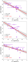 |
Fig. 1. Correlation between metallicity (12 + log(O/H)) and peak magnitude for the three different metallicity estimators (N2 at the top, O3N2 in the middle, and D16 at the bottom). Each Pearson correlation coefficient ρ is shown along with its standard deviation and p value. The best linear fits are shown with the red lines, and the 1σ region is indicated by the gray shades. No host extinction is applied here. |
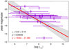 |
Fig. 2. Correlation between the average light-weighted stellar population age (⟨log t*, L⟩) and the peak magnitude. See the caption of Fig. 1 for details. |
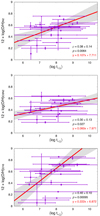 |
Fig. 3. Correlation between the average light-weighted stellar population age (⟨log t*, L⟩) and the metallicity (12 + log(O/H)) for the three different metallicity estimators (N2 at the top, O3N2 in the middle, and D16 at the bottom). See the caption of Fig. 1 for details. |
Pearson correlation coefficients, their standard deviations, and the p values.
It is worth noting that we did not find significant correlations between metallicity and CSM density (Fig. 4). A very weak negative correlation between metallicity and CSM density (i.e., SNe IIn with higher metallicity tend to have a less dense CSM) may exist, but it is still statistically marginal and depends on the metallicity indicator. Interestingly, no positive correlation is likely to exist. Taddia et al. (2015) previously investigated the metallicity dependence of mass-loss rates and wind velocities in SNe IIn. They concluded that SNe IIn from higher-metallicity environments have higher mass-loss rates and wind velocities. Figure 5 shows the CSM density estimates from the SNe IIn used in their analysis. The mass-loss rates and wind velocities in the Taddia et al. (2015) estimates were taken from a range of sources using different methods, and they were not necessarily estimated in a consistent way. Nonetheless, we do not find a significant correlation in the CSM density and metallicity in their sample either. Our results show that although mass-loss rates and wind velocities may have a metallicity dependence as proposed by Taddia et al. (2015), the CSM density (A ∝ Ṁ/vwind) is not significantly metallicity dependent.
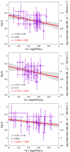 |
Fig. 4. Same as Fig. 1, but for the CSM density (log A*). The right vertical axis shows the corresponding mass-loss rate for a wind velocity of 100 km s−1. |
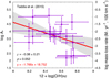 |
Fig. 5. Correlation between metallicity (12 + log(O/H)N2) and CSM density (log A*) for the SN IIn sample in Taddia et al. (2015). The right vertical axis shows the corresponding mass-loss rate for a wind velocity of 100 km s−1. The best linear fitting function (red line) with the 1σ region (gray shade) is shown. |
For the other combinations of the parameters, we do not find any statistically significant correlations. There may be other very weak correlations such as between the rise time and log ΣSFR, between the peak magnitude and log sSFR, and between log A* and ⟨log t*, L⟩. More SNe IIn are required to determine the validity of any additional correlations.
6. Discussion
We found that there is a negative correlation between metallicity and peak luminosity of SNe IIn in the sense that more luminous SNe IIn are associated with lower-metallicity environments. We also found a weak negative correlation between stellar population age and peak luminosity. The luminosity of SNe IIn can be characterized by εEkin/td, where Ekin is the kinetic energy in the shocked SN ejecta up to the time of the luminosity peak (Moriya & Maeda 2014). We found that the rise time, which is related to td, does not correlate with metallicity or stellar age. The conversion efficiency ε is not likely to be sensitive to metallicity and stellar population age, although it could be higher for higher metallicities because the cooling is more efficient. Thus, the negative correlation could be caused by the fact that SNe IIn tend to have a higher explosion energy in lower-metallicity environments and/or younger stellar populations. Because higher-mass progenitors tend to have higher explosion energies (e.g., Martinez et al. 2022), it may be natural to expect SNe IIn from younger stellar populations to have higher explosion energies. However, we do not find any correlations between EW(Hα) and peak luminosity. It is also possible that SN IIn progenitor masses tend to be higher at lower metallicity.
We did not find a significant correlation between metallicity and CSM density. This is interesting because some mass-loss mechanisms predict a positive correlation between mass-loss rate and metallicity. For example, in the case of hot massive stars, Björklund et al. (2021) reported that
![$$ \begin{aligned} \log \left(\frac{\dot{M}}{{M}_\odot \,\mathrm{yr}^{-1}}\right) =&-5.55 + 0.79 \log \left(\frac{Z}{Z_\odot }\right)\nonumber \\&+ \left[2.16-0.32\log \left(\frac{Z}{Z_\odot }\right) \right]\log \left(\frac{L}{10^6\,L_\odot }\right), \end{aligned} $$](/articles/aa/full_html/2023/09/aa46703-23/aa46703-23-eq12.gif)
with vwind ∝ Zp(L) and  . Here, Z is the metallicity and L is the luminosity of a star. This leads to a CSM density factor scaling of

For a given luminosity, the CSM density is expected to correlate positively with the metallicity. In order to have no or negative correlations between A and Z, the SN IIn progenitor luminosity L could increase at low metallicity. Ignoring the small term 0.09log(L/106 L⊙) and assuming L ∝ Zα for SN IIn progenitors, we obtain A ∝ Z1.11 + 2.16α. Thus, α ≲ −0.5 is required to have no or negative correlations between Z and A. If the progenitor luminosity is close to the Eddington luminosity (i.e., L ∝ M), an increase in progenitor mass by a factor of around 2 for a metallicity increase by a factor of 0.3 would produce no correlations, for example.
In the case of cool stars such as red supergiants (RSGs), the metallicity dependence of Ṁ is not so clear. The RSG mass-loss rates have been suggested to follow a relation of Ṁ ∝ L1.05Z0.7 with vwind ∝ L0.35 (Mauron & Josselin 2011, and the references therein), while Goldman et al. (2017) suggested no metallicity dependence for RSG mass-loss rates (Ṁ ∝ L0.9 with vwind ∝ ZL0.4). The two prescriptions predict quite different CSM density dependences on metallicity with A ∝ L0.7Z0.7 (Mauron & Josselin 2011) or A ∝ L0.5Z−1 (Goldman et al. 2017). In both cases, the CSM density around RSGs is predicted to strongly depend on metallicity. Nonetheless, because of the huge uncertainties in the metallicity dependence of RSG mass loss, it is difficult to judge from the metallicity dependence whether SN IIn progenitors are dominated by RSGs. Additional investigations into the metallicity dependence of RSG mass loss are required.
Because of their high mass-loss rates, the progenitors of SNe IIn may have optically thick winds forming a dense CSM. Mass-loss rates and wind velocities from optically thick winds are also predicted to be metallicity dependent, but their dependence may also compensate for a metallicity-independent CSM density (e.g., Gräfener & Hamann 2008; Sander et al. 2020).
It is also possible that the normal mass-loss mechanisms for hot and cool stars are irrelevant for SN IIn progenitors. Their CSM density may be driven by a totally different mass-loss mechanism that is not strongly affected by metallicity. Precursors observed in some SNe IIn (e.g., Ofek et al. 2013; Strotjohann et al. 2021) may indeed indicate that their mass-loss mechanism is quite different from those of the metallicity-dependent steady winds discussed above. For example, continuum-driven winds are not expected to have a metallicity dependence (e.g., Smith & Owocki 2006). Further investigation of the environmental dependence of SN IIn properties would help understanding this unknown mass-loss mechanism in SNe IIn.
Another possibility to explain the apparent lack of a metallicity dependence is that the CSM density depends on the metallicity, but we did not find this clearly because the CSM density needs to be high enough to be observed as SNe IIn. We might simply be biased to SNe with a CSM density above a certain metallicity-independent threshold by observing SNe IIn. In this case, the apparent lack of a metallicity dependence would simply be an observational bias.
7. Conclusions
Using 21 SNe IIn with good light curves and local IFS data, we investigated the relation between local environments and SN properties. We found that SNe IIn with a higher peak luminosity tend to be in environments with lower metallicities and younger stellar population ages. Because metallicity and stellar population age are correlated in our sample, it is unclear whether metallicity, stellar population age, or both drive the correlations. The correlations may indicate that SNe IIn have higher explosion energies in environments with lower metallicity and/or younger stellar ages.
We did not find statistically significant correlations between local metallicity and CSM density around SNe IIn. There might be a very weak negative correlation, but no positive correlation exists. This indicates that the mass-loss mechanism triggering the formation of the dense CSM around SNe IIn could be metallicity independent. Alternatively, the SN IIn progenitor mass range may depend on metallicity. It is also possible that the lack of a metallicity dependence is an observational bias that arose because we established a minimum threshold CSM density for a source to be classified as an SN IIn.
Our study is based on 21 SNe IIn. Some correlations are still not significant, and further confirmation is required. In addition, it is possible that some bias exists in our samples. Thus, a similar study with more SNe IIn is encouraged. Wide-field high-cadence transient surveys are increasing the number of well-observed SNe IIn. Follow-up observations to obtain local environment information to increase the sample size will be important to uncover the mysterious nature of SNe IIn.
Acknowledgments
We thank the anonymous referee for thoughtful comments. This work was supported by the NAOJ Research Coordination Committee, NINS (NAOJ-RCC-2201-0401). T.J.M. is supported by the Grants-in-Aid for Scientific Research of the Japan Society for the Promotion of Science (JP20H00174, JP21K13966, JP21H04997). L.G. acknowledges financial support from the Spanish Ministerio de Ciencia e Innovación (MCIN), the Agencia Estatal de Investigación (AEI) 10.13039/501100011033, and the European Social Fund (ESF) “Investing in your future” under the 2019 Ramón y Cajal program RYC2019-027683-I and the PID2020-115253GA-I00 HOSTFLOWS project, from Centro Superior de Investigaciones Científicas (CSIC) under the PIE project 20215AT016, and the program Unidad de Excelencia María de Maeztu CEX2020-001058-M. H.K. was funded by the Academy of Finland projects 324504 and 328898. J.D.L. acknowledges support from a UK Research and Innovation Fellowship (MR/T020784/1). We acknowledge the Telescope Access Program (TAP) funded by the NAOC, CAS and the Special Fund for Astronomy from the Ministry of Finance. S.D. acknowledges Project number 12133005 supported by National Natural Science Foundation of China (NSFC) and the Xplorer Prize. This work is supported by the Japan Society for the Promotion of Science Open Partnership Bilateral Joint Research Project between Japan and Chile (JPJSBP120209937, JPJSBP120239901). This work was funded by ANID, Millennium Science Initiative, ICN12_009. Based on observations collected at the Centro Astronómico Hispano en Andalucía (CAHA) at Calar Alto, operated jointly by Junta de Andalucía and Consejo Superior de Investigaciones Científicas (IAA-CSIC). Based on observations collected at the European Organisation for Astronomical Research in the Southern Hemisphere under ESO programmes 096.D-0296, 0100.D-0341, 0103.D-0440, 0101.D-0748, 196.B-0578, and 1100.B-0651. This research was partly supported by the Munich Institute for Astro-, Particle and BioPhysics (MIAPbP) which is funded by the Deutsche Forschungsgemeinschaft (DFG, German Research Foundation) under Germany’s Excellence Strategy – EXC-2094 – 390783311. The ZTF forced-photometry service was funded under the Heising-Simons Foundation grant #12540303 (PI: Graham).
References
- Anderson, J. P., James, P. A., Habergham, S. M., Galbany, L., & Kuncarayakti, H. 2015, PASA, 32, e019 [NASA ADS] [CrossRef] [Google Scholar]
- Bacon, R., Vernet, J., Borisova, E., et al. 2014, The Messenger, 157, 13 [NASA ADS] [Google Scholar]
- Barbarino, C., Nyholm, A., & Taddia, F. 2017, Transient Name Server Classification Report, 2017-293, 1 [Google Scholar]
- Björklund, R., Sundqvist, J. O., Puls, J., & Najarro, F. 2021, A&A, 648, A36 [EDP Sciences] [Google Scholar]
- Blanton, M. R., Bershady, M. A., Abolfathi, B., et al. 2017, AJ, 154, 28 [Google Scholar]
- Brimacombe, J., Brown, J. S., Stanek, K. Z., et al. 2016a, ATel, 9344, 1 [NASA ADS] [Google Scholar]
- Brimacombe, J., Brown, J. S., Stanek, K. Z., et al. 2016b, ATel, 9439, 1 [NASA ADS] [Google Scholar]
- Brimacombe, J., Kiyota, S., Holoien, T. W. S., et al. 2016c, ATel, 8703, 1 [NASA ADS] [Google Scholar]
- Brown, J. S., Prieto, J. L., Shappee, B. J., et al. 2016, ATel, 9445, 1 [NASA ADS] [Google Scholar]
- Bundy, K., Bershady, M. A., Law, D. R., et al. 2015, ApJ, 798, 7 [Google Scholar]
- Chandra, P., Chevalier, R. A., James, N. J. H., & Fox, O. D. 2022, MNRAS, 517, 4151 [NASA ADS] [CrossRef] [Google Scholar]
- Chen, P., Dong, S., Kochanek, C. S., et al. 2022, ApJS, 259, 53 [NASA ADS] [CrossRef] [Google Scholar]
- Chevalier, R. A., & Fransson, C. 2006, ApJ, 651, 381 [NASA ADS] [CrossRef] [Google Scholar]
- Cid Fernandes, R., Mateus, A., Sodré, L., Stasińska, G., & Gomes, J. M. 2005, MNRAS, 358, 363 [Google Scholar]
- Cid Fernandes, R., Schoenell, W., Gomes, J. M., et al. 2009, Rev. Mex. Astron. Astrofis. Conf. Ser., 35, 127 [Google Scholar]
- Dong, S., Davis, A. B., Holoien, T. W. S., et al. 2015, ATel, 6864, 1 [NASA ADS] [Google Scholar]
- Dopita, M. A., Kewley, L. J., Sutherland, R. S., & Nicholls, D. C. 2016, Ap&SS, 361, 61 [NASA ADS] [CrossRef] [Google Scholar]
- Elias-Rosa, N., Kromer, M., Faran, T., et al. 2016, ATel, 8727, 1 [NASA ADS] [Google Scholar]
- Filippenko, A. V. 1997, ARA&A, 35, 309 [NASA ADS] [CrossRef] [Google Scholar]
- Fitzpatrick, E. L. 1999, PASP, 111, 63 [Google Scholar]
- Fransson, C., Ergon, M., Challis, P. J., et al. 2014, ApJ, 797, 118 [Google Scholar]
- Galbany, L., Stanishev, V., Mourão, A. M., et al. 2014, A&A, 572, A38 [NASA ADS] [CrossRef] [EDP Sciences] [Google Scholar]
- Galbany, L., Anderson, J. P., Rosales-Ortega, F. F., et al. 2016a, MNRAS, 455, 4087 [NASA ADS] [CrossRef] [Google Scholar]
- Galbany, L., Stanishev, V., Mourão, A. M., et al. 2016b, A&A, 591, A48 [NASA ADS] [CrossRef] [EDP Sciences] [Google Scholar]
- Galbany, L., Anderson, J. P., Sánchez, S. F., et al. 2018, ApJ, 855, 107 [Google Scholar]
- Gal-Yam, A., & Leonard, D. C. 2009, Nature, 458, 865 [NASA ADS] [CrossRef] [Google Scholar]
- Goldman, S. R., van Loon, J. T., Zijlstra, A. A., et al. 2017, MNRAS, 465, 403 [Google Scholar]
- Gräfener, G., & Hamann, W. R. 2008, A&A, 482, 945 [Google Scholar]
- Habergham, S. M., Anderson, J. P., James, P. A., & Lyman, J. D. 2014, MNRAS, 441, 2230 [CrossRef] [Google Scholar]
- Hicken, M., Friedman, A. S., Blondin, S., et al. 2017, ApJS, 233, 6 [NASA ADS] [CrossRef] [Google Scholar]
- Hinshaw, G., Larson, D., Komatsu, E., et al. 2013, ApJS, 208, 19 [Google Scholar]
- Kelz, A., Verheijen, M. A. W., Roth, M. M., et al. 2006, PASP, 118, 129 [Google Scholar]
- Kennicutt, R. C., Jr. 1998, ApJ, 498, 541 [Google Scholar]
- Kiewe, M., Gal-Yam, A., Arcavi, I., et al. 2012, ApJ, 744, 10 [NASA ADS] [CrossRef] [Google Scholar]
- Kochanek, C. S., Shappee, B. J., Stanek, K. Z., et al. 2017, PASP, 129, 104502 [Google Scholar]
- Kumar, B., Eswaraiah, C., Singh, A., et al. 2019, MNRAS, 488, 3089 [NASA ADS] [CrossRef] [Google Scholar]
- Kuncarayakti, H., Galbany, L., Anderson, J. P., Krühler, T., & Hamuy, M. 2016, A&A, 593, A78 [NASA ADS] [CrossRef] [EDP Sciences] [Google Scholar]
- Kuncarayakti, H., Anderson, J. P., Galbany, L., et al. 2018, A&A, 613, A35 [NASA ADS] [CrossRef] [EDP Sciences] [Google Scholar]
- Li, W., Chornock, R., Leaman, J., et al. 2011, MNRAS, 412, 1473 [NASA ADS] [CrossRef] [Google Scholar]
- López-Cobá, C., Sánchez, S. F., Anderson, J. P., et al. 2020, AJ, 159, 167 [Google Scholar]
- Lyman, J., Homan, D., & Yaron, O. 2017, Transient Name Server Classification Report, 2017-937, 1 [Google Scholar]
- Marino, R. A., Rosales-Ortega, F. F., Sánchez, S. F., et al. 2013, A&A, 559, A114 [NASA ADS] [CrossRef] [EDP Sciences] [Google Scholar]
- Martinez, L., Anderson, J. P., Bersten, M. C., et al. 2022, A&A, 660, A42 [NASA ADS] [CrossRef] [EDP Sciences] [Google Scholar]
- Masci, F. J., Laher, R. R., Rusholme, B., et al. 2019, PASP, 131, 018003 [Google Scholar]
- Matzner, C. D., & McKee, C. F. 1999, ApJ, 510, 379 [Google Scholar]
- Mauron, N., & Josselin, E. 2011, A&A, 526, A156 [CrossRef] [EDP Sciences] [Google Scholar]
- Moller, A., Tucker, B., Zhang, B., et al. 2017, Transient Name Server Discovery Report, 2017-923, 1 [Google Scholar]
- Moran, S., Fraser, M., Kotak, R., et al. 2023, A&A, 669, A51 [NASA ADS] [CrossRef] [EDP Sciences] [Google Scholar]
- Moriya, T. J., & Maeda, K. 2014, ApJ, 790, L16 [NASA ADS] [CrossRef] [Google Scholar]
- Moriya, T. J., Maeda, K., Taddia, F., et al. 2014, MNRAS, 439, 2917 [NASA ADS] [CrossRef] [Google Scholar]
- Nyholm, A., Sollerman, J., Tartaglia, L., et al. 2020, A&A, 637, A73 [NASA ADS] [CrossRef] [EDP Sciences] [Google Scholar]
- Ofek, E. O., Rabinak, I., Neill, J. D., et al. 2010, ApJ, 724, 1396 [Google Scholar]
- Ofek, E. O., Sullivan, M., Cenko, S. B., et al. 2013, Nature, 494, 65 [CrossRef] [Google Scholar]
- Ofek, E. O., Arcavi, I., Tal, D., et al. 2014a, ApJ, 788, 154 [NASA ADS] [CrossRef] [Google Scholar]
- Ofek, E. O., Zoglauer, A., Boggs, S. E., et al. 2014b, ApJ, 781, 42 [CrossRef] [Google Scholar]
- Onori, F., Hamanowicz, A., Fraser, M., & Yaron, O. 2017, Transient Name Server Classification Report, 2017-354, 1 [Google Scholar]
- Osterbrock, D. E., & Ferland, G. J. 2006, Astrophysics of Gaseous Nebulae and Active Galactic Nuclei (Sausalito: University Science Books) [Google Scholar]
- Pan, Y. 2017, Transient Name Server Classification Report, 2017-745, 1 [Google Scholar]
- Pastorello, A., Kochanek, C. S., Fraser, M., et al. 2018, MNRAS, 474, 197 [NASA ADS] [CrossRef] [Google Scholar]
- Pessi, P., Csoernyei, G., Holas, A., et al. 2021, Transient Name Server AstroNote, 118, 1 [NASA ADS] [Google Scholar]
- Pessi, T., Anderson, J. P., Lyman, J. D., et al. 2023a, ArXiv e-prints [arXiv:2306.11962] [Google Scholar]
- Pessi, T., Prieto, J. L., Anderson, J. P., et al. 2023b, A&A, in press, https://doi.org/10.1051/0004-6361/202346512 [Google Scholar]
- Pettini, M., & Pagel, B. E. J. 2004, MNRAS, 348, L59 [NASA ADS] [CrossRef] [Google Scholar]
- Poon, H., Pun, J. C. S., Lam, T. Y., Qiu, Y. L., & Wei, J. Y. 2011, ArXiv e-prints [arXiv:1109.0899] [Google Scholar]
- Prieto, J. L., Kistler, M. D., Thompson, T. A., et al. 2008, ApJ, 681, L9 [NASA ADS] [CrossRef] [Google Scholar]
- Ransome, C. L., Habergham-Mawson, S. M., Darnley, M. J., James, P. A., & Percival, S. M. 2022, MNRAS, 513, 3564 [CrossRef] [Google Scholar]
- Reynolds, T., Fraser, M., & Yaron, O. 2016, Transient Name Server Classification Report, 2016-544, 1 [Google Scholar]
- Roth, M. M., Kelz, A., Fechner, T., et al. 2005, PASP, 117, 620 [Google Scholar]
- Sánchez, S. F., Pérez, E., Rosales-Ortega, F. F., et al. 2015, A&A, 574, A47 [NASA ADS] [CrossRef] [EDP Sciences] [Google Scholar]
- Sánchez, S. F., García-Benito, R., Zibetti, S., et al. 2016, A&A, 594, A36 [Google Scholar]
- Sander, A. A. C., Vink, J. S., & Hamann, W. R. 2020, MNRAS, 491, 4406 [Google Scholar]
- Schlegel, E. M. 1990, MNRAS, 244, 269 [NASA ADS] [Google Scholar]
- Shappee, B. J., Prieto, J. L., Grupe, D., et al. 2014, ApJ, 788, 48 [Google Scholar]
- Shappee, B. J., Prieto, J. L., Holoien, T. W. S., et al. 2015, ATel, 6882, 1 [NASA ADS] [Google Scholar]
- Sharma, Y., Sollerman, J., Fremling, C., et al. 2023, ApJ, 948, 52 [NASA ADS] [CrossRef] [Google Scholar]
- Smith, N. 2014, ARA&A, 52, 487 [NASA ADS] [CrossRef] [Google Scholar]
- Smith, N., & Andrews, J. E. 2020, MNRAS, 499, 3544 [NASA ADS] [CrossRef] [Google Scholar]
- Smith, N., & Owocki, S. P. 2006, ApJ, 645, L45 [NASA ADS] [CrossRef] [Google Scholar]
- Smith, K. W., Smartt, S. J., Young, D. R., et al. 2020, PASP, 132, 085002 [Google Scholar]
- Sorce, J. G., Tully, R. B., Courtois, H. M., et al. 2014, MNRAS, 444, 527 [Google Scholar]
- Springob, C. M., Magoulas, C., Colless, M., et al. 2014, MNRAS, 445, 2677 [Google Scholar]
- Strotjohann, N. L., Ofek, E. O., Gal-Yam, A., et al. 2021, ApJ, 907, 99 [NASA ADS] [CrossRef] [Google Scholar]
- Taddia, F., Stritzinger, M. D., Sollerman, J., et al. 2013, A&A, 555, A10 [NASA ADS] [CrossRef] [EDP Sciences] [Google Scholar]
- Taddia, F., Sollerman, J., Fremling, C., et al. 2015, A&A, 580, A131 [NASA ADS] [CrossRef] [EDP Sciences] [Google Scholar]
- Takats, K., Rodriguez, O., Galbany, L., & Yaron, O. 2016, Transient Name Server Classification Report, 2016-932, 1 [Google Scholar]
- Theureau, G., Hanski, M. O., Coudreau, N., Hallet, N., & Martin, J. M. 2007, A&A, 465, 71 [NASA ADS] [CrossRef] [EDP Sciences] [Google Scholar]
- Tonry, J., Denneau, L., Stalder, B., et al. 2016, Transient Name Server Discovery Report, 2016-909, 1 [Google Scholar]
- Tonry, J., Stalder, B., Denneau, L., et al. 2017a, Transient Name Server Discovery Report, 2017-284, 1 [Google Scholar]
- Tonry, J., Stalder, B., Denneau, L., et al. 2017b, Transient Name Server Discovery Report, 2017-336, 1 [Google Scholar]
- Tonry, J., Stalder, B., Denneau, L., et al. 2017c, Transient Name Server Discovery Report, 2017-709, 1 [Google Scholar]
- Tonry, J. L., Denneau, L., Heinze, A. N., et al. 2018, PASP, 130, 064505 [Google Scholar]
- Tonry, J., Denneau, L., Heinze, A., et al. 2021, Transient Name Server Discovery Report, 2021-771, 1 [Google Scholar]
- Tsuna, D., Kashiyama, K., & Shigeyama, T. 2019, ApJ, 884, 87 [NASA ADS] [CrossRef] [Google Scholar]
- Tully, R. B., Courtois, H. M., Dolphin, A. E., et al. 2013, AJ, 146, 86 [NASA ADS] [CrossRef] [Google Scholar]
- Van Dyk, S. D., Peng, C. Y., King, J. Y., et al. 2000, PASP, 112, 1532 [NASA ADS] [CrossRef] [Google Scholar]
- Verheijen, M. A. W., Bershady, M. A., Andersen, D. R., et al. 2004, Astron. Nachr., 325, 151 [Google Scholar]
- Weis, K., & Bomans, D. J. 2020, Galaxies, 8, 20 [NASA ADS] [CrossRef] [Google Scholar]
- Willick, J. A., & Batra, P. 2001, ApJ, 548, 564 [NASA ADS] [CrossRef] [Google Scholar]
- Xu, Z., Li, B., Li, Z., et al. 2017, Transient Name Server Discovery Report, 2017-903, 1 [Google Scholar]
Appendix A: Figures of the SN environments
We present supplementary figures presenting each SN environment. Figure A.1 shows SN host galaxies with SN locations, and Fig. A.2 shows their spectra, which were used to estimate the SN environment parameters.
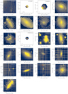 |
Fig. A.1. SN IIn host galaxies in the synthesized r band in our IFS data. The red circle is the SN position with the seeing-sized aperture. |
 |
Fig. A.2. Spectra of the SN IIn environments used for the environmental parameter estimations. Gray, red, and blue spectra are aperture spectra, the best SSP fits, and their resulting gas-pahse emissioin spectra, respectively. |
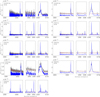 |
Fig. A.2. continued. |
Appendix B: Light-curve fitting results
The results of light-curve fitting that were used to estimate the rise time and peak luminosity of our SN IIn sample are presented in Fig. B.1. The fitting formula is Eq. (11).
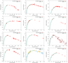 |
Fig. B.1. Light curves and fits for the SNe IIn. The light-curve fit to the peak is presented, and the peak is where the fitted line ends. |
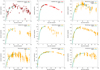 |
Fig. B.1. continued. |
All Tables
All Figures
|
Fig. 1. Correlation between metallicity (12 + log(O/H)) and peak magnitude for the three different metallicity estimators (N2 at the top, O3N2 in the middle, and D16 at the bottom). Each Pearson correlation coefficient ρ is shown along with its standard deviation and p value. The best linear fits are shown with the red lines, and the 1σ region is indicated by the gray shades. No host extinction is applied here. |
| In the text | |
|
Fig. 2. Correlation between the average light-weighted stellar population age (⟨log t*, L⟩) and the peak magnitude. See the caption of Fig. 1 for details. |
| In the text | |
|
Fig. 3. Correlation between the average light-weighted stellar population age (⟨log t*, L⟩) and the metallicity (12 + log(O/H)) for the three different metallicity estimators (N2 at the top, O3N2 in the middle, and D16 at the bottom). See the caption of Fig. 1 for details. |
| In the text | |
|
Fig. 4. Same as Fig. 1, but for the CSM density (log A*). The right vertical axis shows the corresponding mass-loss rate for a wind velocity of 100 km s−1. |
| In the text | |
|
Fig. 5. Correlation between metallicity (12 + log(O/H)N2) and CSM density (log A*) for the SN IIn sample in Taddia et al. (2015). The right vertical axis shows the corresponding mass-loss rate for a wind velocity of 100 km s−1. The best linear fitting function (red line) with the 1σ region (gray shade) is shown. |
| In the text | |
|
Fig. A.1. SN IIn host galaxies in the synthesized r band in our IFS data. The red circle is the SN position with the seeing-sized aperture. |
| In the text | |
|
Fig. A.2. Spectra of the SN IIn environments used for the environmental parameter estimations. Gray, red, and blue spectra are aperture spectra, the best SSP fits, and their resulting gas-pahse emissioin spectra, respectively. |
| In the text | |
|
Fig. A.2. continued. |
| In the text | |
|
Fig. B.1. Light curves and fits for the SNe IIn. The light-curve fit to the peak is presented, and the peak is where the fitted line ends. |
| In the text | |
|
Fig. B.1. continued. |
| In the text | |
Current usage metrics show cumulative count of Article Views (full-text article views including HTML views, PDF and ePub downloads, according to the available data) and Abstracts Views on Vision4Press platform.
Data correspond to usage on the plateform after 2015. The current usage metrics is available 48-96 hours after online publication and is updated daily on week days.
Initial download of the metrics may take a while.