| Issue |
A&A
Volume 677, September 2023
|
|
|---|---|---|
| Article Number | A148 | |
| Number of page(s) | 23 | |
| Section | Interstellar and circumstellar matter | |
| DOI | https://doi.org/10.1051/0004-6361/202245522 | |
| Published online | 21 September 2023 | |
SiO outflows in the most luminous and massive protostellar sources of the southern sky
1
Departamento de Astronomia, Universidad de Chile,
Santiago, Chile
e-mail: nguerra@ug.uchile.cl
2
Dipartimento di Fisica, Università di Roma “Tor Vergata”,
Via della Ricerca Scientifica 1,
00133
Roma, Italy
3
Department of Astronomy, University of Belgrade – Faculty of Mathematics,
Studentski trg 16,
11000
Belgrade, Serbia
4
Instituto de Astrofisica de La Plata (UNLP-CONICET),
La Plata, Argentina
5
Faculdad de Ciencias Astronomicas y Geofisicas, Universidad Nacional de La Plata,
Paseo del Bosque s/n,
1900,
La Plata, Argentina
6
INAF – IAPS,
Via Fosso del Cavaliere, 100,
00133
Roma, Italy
7
Dept. Ciencias Integradas, Facultad de Ciencias Experimentales, Centro de Estudios Avanzados en Fisica, Matemática y Computación, Unidad Asociada GIFMAN, CSIC-UHU, Universidad de Huelva,
Spain
Received:
21
November
2022
Accepted:
17
July
2023
Context. High-mass star formation is far less understood than low-mass star formation. It entails the ejection of matter through molecular outflows, which disturbs the protostellar clump. Studying these outflows and the shocked gas caused by them is the key to a better understanding of this process.
Aims. The present study aims to characterise the behaviour of molecular outflows in the most massive protostellar sources in the southern Galaxy by looking for evolutionary trends and associating the presence of shocked gas with outflow activity.
Methods. We present APEX SEPIA180 (Band 5) observations (beamwidth ~36″) of SiO(4-3) molecular outflow candidates towards a well-selected sample of 32 luminous and dense clumps, which are candidates for harbouring hot molecular cores. We study the emission of the SiO(4-3) line, which is an unambiguous tracer of shocked gas, and recent and active outflow activity, as well as the HCO+(2-1) and H13CO+(2-1) lines.
Results. Results show that 78% of our sample (25 sources) present SiO emission, revealing the presence of shocked gas. Nine of these sources are also found to have wings in the HCO+(2-1) line, indicating outflow activity. The SiO emission of these nine sources is generally more intense (Ta > 1 K) and wider (~61 km s−1 FWZP) than the rest of the clumps with SiO detection (~42 km s−1 FWZP), suggesting that the outflows in this group are faster and more energetic. This indicates that the shocked material gets dispersed as the core evolves and outflow activity decreases. Three positive linear correlations are found: a weak one (between the bolometric luminosity and outflow power) and two strong ones (one between the outflow power and the rate of matter expulsion and the other between the kinetic energy and outflow mass). These correlations suggest that more energetic outflows are able to mobilise more material. No correlation was found between the evolutionary stage indicator L/M and SiO outflow properties, supporting that molecular outflows happen throughout the whole high-mass star formation process.
Conclusions. We conclude that sources with both SiO emission and HCO+ wings and sources with only SiO emission are in an advanced stage of evolution in the high-mass star formation process, and there is no clear evolutionary difference between them. The former present more massive and more powerful SiO outflows than the latter. Therefore, looking for more outflow signatures such as HCO+ wings could help identify more massive and active massive star-forming regions in samples of similarly evolved sources, and could also help identify sources with older outflow activity.
Key words: stars: formation / stars: massive / ISM: clouds / ISM: jets and outflows / ISM: molecules
© The Authors 2023
 Open Access article, published by EDP Sciences, under the terms of the Creative Commons Attribution License (https://creativecommons.org/licenses/by/4.0), which permits unrestricted use, distribution, and reproduction in any medium, provided the original work is properly cited.
This article is published in open access under the Subscribe to Open model. Subscribe to A&A to support open access publication.
1 Introduction
Massive stars are crucial to the evolution of the interstellar medium (ISM) and galaxies. However, they are difficult to observe and study because they are very scarce (about 1% of stellar populations), have short timescales and large heliocentric distances, and are embedded in very complex environments with high extinction and turbulence (e.g. Motte et al. 2018). Thus, high-mass star formation remains much less understood than low-mass star formation.
The current picture for high-mass star formation is that it takes place in massive dense cores (MDCs) embedded in massive clouds called massive star-forming (MSF) regions, and can be described by four main phases (van der Tak 2004; Motte et al. 2018; Elia et al. 2021; Urquhart et al. 2022; Jiao et al. 2023). Initially, in the quiescent or starless phase, the clump has no embedded objects and is not visible at 70 μm. Later, in the young stellar object (YSO) phase, the clump has warmed up enough to be detected at 70 μm In this stage, (~104 yr), there is an embedded cold and collapsing prestellar core. When a protostar appears (protostellar phase, ~3 × 10⁵ yr), it feeds on inflow material and its mass increases until it becomes a high-mass protostar. Within this phase, the hot molecular core (HMC) stage can be identified. Then, as the protostar evolves and its temperature increases, it starts emitting ultraviolet (UV) radiation, which quickly ionises the surrounding gas. This starts the ultra-compact (UC) HII region phase (~105−106 yr).
Massive star formation entails a greatly relevant feedback process: molecular outflows and jets (i.e. matter expulsion at high velocities due to angular momentum conservation during matter accretion; Arce et al. 2007; Bally 2016; Motte et al. 2018). This feedback process occurs throughout the whole of the high-mass formation process (Li et al. 2020; Yang et al. 2022; Urquhart et al. 2022), and outflow features have been used as an indication of massive star formation activity (Li et al. 2019c; Liu et al. 2020). In order to understand how massive stars form, the study of molecular outflows in MSF regions is imperative.
The study of outflows heavily depends on the tracer used. There is no such thing as a perfect outflow tracer (Bally 2016). However, the SiO molecule has been found to be a very good tracer of outflow activity and shocked material, and has been broadly used for this purpose (e.g. Beuther et al. 2002; López-Sepulcre et al. 2011; Bally 2016; Li et al. 2019b; Liu et al. 2021a,b, 2022; De Simone et al. 2022). Silicon falls onto the icy mantles of the dust grains of the ISM. When hit by shocks of gas, the dust grains can sublimate to the gaseous state, releasing the Si. Thus, the Si in the gas phase can react with oxygen to form SiO, making it observable in the millimetre (mm), sub-mm, and centimetre (cm) regimes via its rotational transitions (Schilke et al. 1997; Klaassen & Wilson 2007; Gusdorf et al. 2008). Unlike other molecules, SiO has a key advantage. Its emission is not easily contaminated by excited ambient material, which makes it an unambiguous tracer of shocked material, and thus of outflow activity. Studying SiO emission can shed light on the kinematics of outflows and on the relevant chemical processes that occur in shock environments, such as the formation of complex organic molecules (COMs; Bally 2016; Li et al. 2020; Rojas-García et al. 2022). Broad spectral width SiO emission (full width zero power, FWZP ≥ 20 km s−1) and narrow spectral width SiO emission (FWZP ≤ 10 km s−1) have both been observed (Garay et al. 2010; Leurini et al. 2014; Bally 2016; Csengeri et al. 2016; Li et al. 2019b; Zhu et al. 2020). It is thought that broad-width emission is due to high-velocity col-limated shocks, while narrow-width emission is associated with less collimated low-velocity shocks, such as cloud-cloud collisions. It is possible to identify wings in the SiO spectral profile when it has a broad width, which are manifestations of SiO outflows. These have been extensively studied (Beuther et al. 2002; Liu et al. 2021a,b). Moreover, SiO outflow activity has been found to decrease and become less collimated over time (Arce et al. 2007; Sakai et al. 2010; López-Sepulcre et al. 2011). However, there is currently no consensus on whether SiO abundance decreases over time (Csengeri et al. 2016; Li et al. 2019b; Liu et al. 2022), and some works even conclude that SiO emission is much harder to interpret than just as a shock tracer (Widmann et al. 2016).
Another very helpful outflow tracer is HCO+ emission (Myers et al. 1996; Rawlings et al. 2004; Klaassen & Wilson 2007; Bally 2016; Li et al. 2019a; Liu et al. 2020; He et al. 2021). This species traces the surrounding material of protostar regions (Rawlings et al. 2004) and traces the disk material in low-mass star formation (Dutrey et al. 1997). This species can trace both inflow and outflow motions (Klaassen & Wilson 2007). When outflows are strong enough, they can be observed in broad high-velocity wings in the spectral profile (Wu et al. 2005; He et al. 2021). When HCO+, and other species such as CO, are dragged outwards due to the outflow, their spectral profiles present wings. This is caused by the greater velocity gradient of the dragged material. However, the spectral profile of this species experiences significant absorption, which often complicates its analysis. Moreover, studying the emission of an HCO+ isotopologue, H13CO+, can help distinguish between outflows and ambient dense gas as it traces dense gas only (see Sect. 3.1).
SiO line emissions are associated with recent and active outflow of matter, as shock chemistry processes happen in 102–104 yr, whilst the HCO+ wing observations are associated with old ‘fossil’ outflows (Arce et al. 2007; Klaassen & Wilson 2007; López-Sepulcre et al. 2016; Li et al. 2019a). The detection of only one of these phenomena is enough to indicate the presence of a molecular outflow. If both are detected, then it is possible to confirm without ambiguity that there is ongoing matter expulsion (Klaassen & Wilson 2007). Outflows are associated with an advanced stage of evolution. If a molecular core does not have an outflow, it may be because it has not reached this point yet. However, it is also possible that it has already experienced a significant loss of material and/or that accretion and outflow activity have ceased.
In this work we present SiO(2-1), HCO+(2-1), and H13CO+(2-1) APEX Band 5 observations towards a well-selected sample of 32 very massive and luminous protostellar sources that are amongst the brightest clumps in the Southern Milky Way. This study addresses several research questions, including how SiO outflows behave in the most massive proto-stellar sources, whether the presence of shocked gas is associated with outflow activity, and what different outflow signatures can tell us about similarly evolved sources.
This paper is organised as follows. In Sect. 2 we describe the studied sample, the selection criteria, and the observations. In Sect. 3 we analyse the data and describe how outflow and SiO detections were analysed. In Sect. 4 we calculate the outflow properties of the clumps and the SiO emission. In Sect. 5 we present relevant correlations, carry out a cross-check between SiO and outflow detections, and discuss possible evolutionary trends. Finally, in Sect. 6 we provide a summary of our main results and present our conclusions.
2 Observations
2.1 Source selection
The studied sample consists of 32 protostellar clumps (HMC candidates) from the Hi-GAL catalogue of compact sources (Elia et al. 2021), associated with CS(2-1) line emission from IRAS PSC sources with far-infrared colours of Ultra Compact HII regions by Bronfman et al. (1996). Their characteristics are presented in Table 1; the sources flagged with a black diamond (♦) have saturated Hi-GAL observations (see Appendix A). The sources have been given an identifier consisting of ‘HC’ (hot core) plus a number, and are listed in increasing order for convenience. The sources were selected using the following criteria:
Kinematic distance <6 kpc (from Reid et al. 2009; Hi-GAL distances were not used; see Appendix B);
Strong CS emission (Bronfman et al. 1996): Main-beam temperature in CS TMB(CS) ≥1.5 K;
Surface density above the threshold for the formation of massive stars: Σ > 0.2 g cm−2 (e.g. Butler & Tan 2012; Merello et al. 2018);
Mass >100 M⊙ (Elia et al. 2021);
High luminosity-to-mass ratio L/M. Values of this evolutionary stage indicator higher than 1 are associated with internal protostellar heating and the appearance of new stars in massive clumps (López-Sepulcre et al. 2011; Molinari et al. 2016).
Although low-mass star-forming clumps may also have a high value of L/M, the lower limit set on the mass of the clump together with a high L/M ensures our sample will only consist of massive protostellar clumps.
The sources in our sample are at an advanced stage of evolution, either in the protostellar or compact HII region phase. A histogram of the luminosity-to-mass ratio L/M, which acts as an evolutionary stage indicator, is presented in Fig. 1 (see Table 1). The parameter L/M has a minimum value of 3 L⊙/M⊙, a maximum of 154 L⊙/M⊙, a mean of 45 L⊙/M⊙, and a median of 30 L⊙/M⊙.
The sources are very energetic, with bolometric luminosities up to ~2.3 × 10⁵L⊙. The selection criteria of the sources allowed us to work only with luminous, strong, and relatively near clumps. They are among the most luminous sources in the southern sky, and some of them have been extensively studied (see Appendix C). The continuum dust properties of the sources are shown in Table 2; the sources flagged with a black diamond (♦) have saturated Hi-GAL observations (see Appendix A) and were obtained from a SED fit (Elia et al. 2021). Compared with the general population of Hi-GAL protostellar sources (Elia et al. 2017, 2021), we see that our sample is much more massive and luminous. The median value for H2 mass derived from dust Mdust and bolometric luminosity LBol for our sample is 828 M⊙ and 19839 L⊙, respectively, whilst for Hi-GAL protostellar sources these values are equal to 464 M⊙ and 1071 L⊙, respectively. In comparison with the rest of the Hi-GAL sources within 6 kpc, the contrast is even greater since the mean bolometric luminosity is 206 L⊙ and the mean dust mass is 88 M⊙ in this region of the Galaxy. Finally, Fig. 2 shows the distribution in the Galactic plane of the sources presented in this work.
Studied sample sources.
2.2 APEX observations
Observations were made using the SEPIA180 instrument at the Atacama Pathfinder Experiment (APEX)1 in the Atacama Desert in Chile (Belitsky et al. 2018) for ten nights between November 2018 and October 2019. The observations were made in single-pointing mode. For each source a region free from emission was taken as reference from the dust maps at 250 μm by Herschel, typically at 300–500″ from the source. The system temperature was 174.30 K on average.
The band was tuned at 172 GHz in the LSB to observe the H13CO+(2-1) (173.507 GHz) and SiO(4-3) (173.688 GHz) lines, and centred at the HCO+(2−l) line (178.375 GHz). The spectral resolution used was of ∆V = 0.2 km s−1, which gives a typical RMS noise temperature of 25 mK, and the main beam efficiency ηMB was equal to 0.83. APEX observations have an antenna temperature uncertainty of about 20% (APEX staff, priv. comm.). The frequency of the transitions used was obtained from the SPLATALOGUE2 database. This frequency range corresponds to Band 5 of the Atacama Large Millimeter/submillimeter Array.
The beam angular size can be calculated with the frequency f of a spectral line with θ″ = 7.8″ × 800/f. For these observations this results in a beam angular size of approximately 36″.
The CLASS software from the GILDAS3 software package was used to reduce the spectra. It is used to process single-dish spectra and is oriented towards the processing of a large number of spectra. For every spectral line, the baseline was subtracted at first order and then centred to the VLSR of the corresponding source.
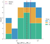 |
Fig. 1 Histogram of the luminosity-to-mass ratio L/M in logarithmic scale. The red and purple vertical lines denote the median (30 L⊙/M⊙) and the mean (45 L⊙/M⊙), respectively. Groups A, B, and C are defined in Table 6. |
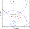 |
Fig. 2 Galactic distribution of the sources. The orange point corresponds to the Sun and the green point to the Galactic centre. The red crosses are the sources studied in this paper. The blue circles are centred on the Sun and the black circles on the Galactic centre. They indicate the 1, 5, and 10 kpc distances. |
Clump properties.
3 Analysis
The SiO(4-3), H13CO+(2-1), and HCO+(2-1) spectral profiles of source HC02 are presented in Fig. 3 as an example, where the red dotted line is at FWZP and the blue line in the H13CO+ panel shows the Gaussian fit (see Figs D.1–D.31 for the rest).
Results for the HCO+(2-1), H13CO+(2-1), and SiO(4-3) spectral lines are displayed in Tables 3–5, respectively. We calculated the spatial beam size R with the angular beam size θ and distance to the source D:
 (1)
(1)
It should be noted that since our observations do not resolve the singular clump, the spatial beam size is diluted and introduces uncertainties. We compared the beam size of the sources at the H13CO+ (2-1) line with their beam-deconvolved sizes measured at 250 μm continuum emission obtained from the Hi-GAL catalogue of compact sources (Elia et al. 2021). The H13CO+ line traces the cold surrounding material; on the other hand, the cold dust is expected to emit at around 250 μm (i.e. they trace mostly the same dense gas; e.g. Elia et al. 2017). Thus, we computed the ratio of the clump sizes in 250 μm to those in the H13CO+ (2-1) line. This indicates how beam dilution affects our results. We found that the beam size in our APEX observations is on average 2.35 times larger than the size of the clump at 250 μm On the other hand, the SiO(4-3) line has an angular resolution of 36″, which corresponds to 0.087 pc at a distance of 1 kpc. The distances to our sources range from 1.33 to 5.54 kpc. These uncertainties propagate linearly to the column densities to be calculated in Sect. 4.1.2.
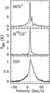 |
Fig. 3 Spectral profiles for source HC02, Group A. The red dotted line is at FWZP and the blue line in the H13CO+ panel shows the Gaussian fit. |
3.1 Clump tracer emission
The HCO+ and H13CO+ species are commonly used as dense gas tracers. They are treated as linear rigid rotors (Mladenović 2017) and are expected to present a Gaussian profile. Although they are isotopologues, these lines present different behaviours. At a kinetic temperature of 20 K, the HCO+(2-1) and H13CO+(2-1) lines have optically thin critical densities of 4.2 × 105 cm−3 and 3.8 × 105 cm−3 and effective excitation densities of 1.7 × 103 cm−3 and 7.1 × 104 cm−3, respectively (Shirley 2015). The HCO+ has a much lower effective density than its isotopologue, which indicates that HCO+ traces regions with lower density, such as outflows and jets, which are usually less dense than the surrounding material. This is why HCO+ traces both outflows and the surrounding material, whilst H13CO+ only traces the latter. The differences between these two lines are visually clear in their spectral profiles (see Fig. 3 and Appendix D). HCO+ emission experiences significant absorption and self-absorption (Klaassen & Wilson 2007), and thus it is not possible to quantify properties of the clump using this spectral profile only. In addition, H13CO+ emission is optically thin and does not present absorption. Therefore, the Gaussian parameters fitted to the H13CO+(2-1) spectral profiles were used to calculate the properties of the cores for all the sources, and the velocity of the H13CO+(2-1) Gaussian peak was used to centre the standard of rest velocity VLSR of the sources. The parameters of the HCO+(2-1) spectral lines are displayed in Table 3, and the results from the Gaussian fit to the H13CO+(2-1) spectral profile are displayed in Table 4.
We note that if the outflow is strong enough, it is possible that the H13CO+ line presents wings as well, as is the case for source HC20 (see Fig. D.19). Since the sources in our sample are extreme, it is reasonable to see this feature. The wings in the H13CO+ line are much smaller than those in the HCO+ line, and it is still possible to properly fit a Gaussian curve.
Since wings in the HCO+ spectral profile are a very good indicator of outflows, its (2-1) spectral line was used to determine the presence of molecular outflows through the detection of wings. In the literature, spectral lines with wings are usually modelled by a Lorentz distribution. However, this line presents significant absorption in our data, which makes any curve fit far too inaccurate. Thus, HCO+ wings were checked in the following way. The sum of the widths of the red and blue wings was obtained by subtracting the baseline width of the Gaussian fit of the H13CO+ line from the HCO+ FWZP. If the sum of the widths was larger than 25 km s−1, then the given source was deemed to have HCO+ wings. As modelled by Gusdorf et al. (2008; see also Leurini et al. 2014), shocks trigger the erosion of grains, and SiO can be efficiently produced only if shock speeds are above 25 km s−1. Results show (see Table 3) that 28% of our sample (nine sources) present wings in the HCO+ spectral profile (see e.g. Fig. D.7). However, we note that, due to the lack of spatial information, there is significant uncertainty in these results.
HCO+ spectral line data.
H13CO+ spectral line data.
3.2 SiO detection
We checked whether the sources present SiO emission, which directly traces outflows and shocked gas. Emission at 5σ or more was considered. SiO emission was found in 78% of our sample (25 sources). The results are displayed in Table 5.
The material ejected by bipolar outflows forms two lobes, as modelled in Rawlings et al. (2004). Depending on the inclination angle, this produces two main features: the red and blue wings. While centred at the velocity of each source, the width from the Gaussian fit to the H13CO+(2-1) line was subtracted from the SiO(4-3) spectral profile width to obtain the width of the red and blue wings. With these measurements (see Table 5) the velocity integrated intensity of the SiO wings were obtained and further used to calculate the physical properties of the outflows.
There are a few sources that have particularly intense SiO emission, such as source HC02 (associated with IRAS 17574−2403). The peak of the emission of these sources is ≥20 times the RMS and they have Tpeak > 0.7 K. A more detailed description and summary of previous works done on these sources can be found in Appendix C. According to our results, we divided the sample into three groups, as seen in Table 6: 9 sources present both SiO detection and HCO+ wings, 16 sources present SiO emission and no HCO+ wings, and the remaining 7 present neither.
SiO spectral line data.
Grouping of the sources.
4 Results
4.1 Properties of the clump
4.1.1 Virial masses
The Gaussian width of the H13CO+(2-1) spectral line was used to calculate the virial mass of the clump. Assuming that it is grav-itationally bound, so that the virial theorem applies, the virial mass can be calculated as (e.g. Merello et al. 2013)
 (2)
(2)
where ∆V is the line’s Gaussian width and R is the spatial beam size of the source.
The results show (see Table 7) that these sources have very high virial masses, reaching up to 4.9 × 10³M⊙. However, the beam of the observation instrument APEX is larger than the clump, and thus the observations include more material.
4.1.2 LTE mass
The local thermodynamic equilibrium (LTE) mass of the clump was calculated using the LTE formalism, assuming the emission is optically thin. The H13CO+ is a linear and rigid rotor molecule. Thus, the column density NJ was calculated as follows (e.g. Garden et al. 1991; Sanhueza et al. 2012):
![$\matrix{ {{N_J} = {{3h} \over {8{\pi ^3}\,{{\rm{\mu }}^2}\,}}{{U\left( {{T_{{\rm{ex}}}}} \right)} \over {\left( {J + 1} \right)}}{{\exp \,\left( {{{{E_J}} \over {k{T_{{\rm{ex}}}}}}} \right)} \over {\left[ {1 - \exp \,\left( {{{ - hv} \over {k{T_{{\rm{ex}}}}}}} \right)} \right]}}} \hfill \cr {\,\,\,\,\,\,\,\,\,\,\,\,\,\, \times {1 \over {\left( {J\left( {{T_{{\rm{ex}}}}} \right) - J\left( {{T_{{\rm{bg}}}}} \right)} \right)}}\int {\,{T_{{\rm{MB}}}}{\rm{d}}v.} } \hfill \cr } $](/articles/aa/full_html/2023/09/aa45522-22/aa45522-22-eq3.png) (3)
(3)
Here, k is the Boltzmann constant, h is the Planck constant, μ = 3.89 × 10⁻¹⁸ (D) is the electric dipole momenta, and EJ = hBJ(J + 1) is the energy in the level J (in this case, J = 1), where B = 43377.165 (MHz) is the rotational constant. The intensity J(T) is defined for a given frequency ν as
 (4)
(4)
Finally, U (T) is the partition function
![$U\left( T \right) = \sum\limits_{J = 0}^\infty {{g_J}\,\exp \,\left[ {{{ - hBJ\left( {J + 1} \right)} \over {k{T_{{\rm{ex}}}}}}} \right] \approx {k \over {hB}}\,\left( {{T_{{\rm{ex}}}} + {{hB} \over {3k}}} \right)} ,$](/articles/aa/full_html/2023/09/aa45522-22/aa45522-22-eq5.png) (5)
(5)
where ɡJ = 2J + 1 is the rotational degeneracy. A cosmic background temperature Tbg of 2.75 K was considered. The excitation temperature Tex was set to a standard value of 30 K, which is close to the median of the dust temperatures (26.4 ± 6.0 K; e.g. Elia et al. 2017). The total column density in units of cm−2 can be obtained by multiplying NJ by the abundance of H13CO+: [H2/H13CO+] = 3.0 × 10¹⁰ (Blake et al. 1987). Finally, the LTE mass was obtained by multiplying the total column density by the area of the source,
 (6)
(6)
where R is the radius of the beam. These results are also shown in Table 7.
We compared our LTE mass estimates to the clump mass derived from dust emission obtained by Hi-GAL (Elia et al. 2017, 2021). The ratio of the dust to LTE masses has a mean of 2.11, a median of 1.64, and a standard deviation of 1.34. The origin of this uncertainty can come from the assumed temperature and from the H13CO+ abundance. Furthermore, the dust masses from Hi-GAL used here were calculated by fitting a spectral energy distribuiton (SED) which was scaled to the angular size at 250 μm (Elia et al. 2013; Motte et al. 2010). We note that for the four saturated sources of the sample, the mass used here was obtained using the flux at 500 μm instead (see Appendix A for the treatment of saturated sources). The H13CO+ line and emission at 250 μm trace mostly the same dense gas, and their angular sizes are within a factor of 2.35 on average (see Sect. 3), which is consistent with the difference seen between the masses. This indicates that our estimates are sound.
The uncertainty of the molecular observations is ~20%, which affects the Gaussian fit parameters, and propagates to the rest of the clump’s properties. Because of the propagating error, the column density can be considered to have an uncertaintly of 10–20%, whilst the mass uncertainty is <30%. The distances are also a source of uncertainty, which affects the beam radius and masses (see Appendix B).
Properties obtained from H13CO+ emission.
4.1.3 Virial and LTE mass comparison
The ratio of the virial to LTE mass can provide information about the gravitational stability of the source. High values of this ratio indicate that the internal kinetic energy of the source is too high, and that it is not massive enough to be gravitationally stable. Since the material traced by H13CO+ emission should be both gravitationally bound and in local thermodynamic equilibrium, the virial and LTE mass should match within a factor of ~2 when magnetic effects are not considered. Results are presented in Table 7. The ratio of the virial to LTE mass has a mean value of 1.54, a median of 1.45, a minimum of 0.64, and a maximum of 3.07. Only eight sources have a ratio of 2.00 or higher. Thus, the virial and LTE masses are in good agreement.
4.2 Properties of the SiO outflows
4.2.1 Outflow mass
We calculated the LTE mass for the SiO outflows in the red and blue wings. With an assumption of optically thin thermal SiO(4-3) emission in LTE (e.g. Liu et al. 2021a), the column densities NJ and Ntot and the LTE mass were calculated as described in Sect. 4.1.2 using a rotational constant B of 21711.96 (MHz), an electric dipole moment μ of 3.10 × 10⁻¹⁸ (D), an excitation temperature Tex of 18 K, and an SiO abundance [H2/SiO] of 109 (Liu et al. 2021a; Sanhueza et al. 2012), standard values for this source type. If a higher Tex of 25 K or 30 K were used, the values of the outflow masses would increase by 16.32 and 29.42%, respectively. Since SiO abundances can drastically vary in different MSF regions (by up to six orders of magnitude; Ziurys et al. 1989; Martin-Pintado et al. 1992; Li et al. 2019b), using an inadequate choice for this parameter could artificially modify the results. Here we use a standard value for [H2/SiO], accepted for protostellar objects. The results are displayed in Table 8.
4.2.2 Dynamical properties
We obtained further characteristics of the outflow (Beuther et al. 2002): momentum Pout, kinetic energy Ekin, characteristic timescale t, mechanical force or flow of momentum F, rate of matter expulsion Ṁ, and mechanical luminosity or power Lm.
They were computed as follows:
 (7)
(7)
 (8)
(8)
 (9)
(9)
 (10)
(10)
 (11)
(11)
 (12)
(12)
Here, R is the radius of the source, Mout = Mr + Mb is the total outflow mass, and Vb and Vr are the maximum velocities of the outflows, which correspond to |VLSR – Vi |(Beuther et al. 2002; Liu et al. 2021b), where Vi is the velocity at each extreme of the SiO emission baseline. The results are displayed in Table 8.
The uncertainty of the observations (20%; see Sect. 2.2) propagates to these calculated properties. The outflow column density and mass have uncertainties of about 10–20% and <30%, respectively. The momentum and kinetic energy have the same uncertainty as the mass, whilst the force, rate of matter expulsion, and mechanical luminosity have an additional source of uncertainty due to the dynamical timescales, which comes from the distances and the instrumental error (~20%).
A statistical description of these results is shown in Table 9. The typical rate of matter expulsion for mid and early massive protostars ranges from 10−5 to a few times 10−3 M⊙ yr−1, and the typical momentum from 10−4 to 10−2 M⊙ km s−1 (Arce et al. 2007). Our results for the rate of matter expulsion are well within this typical range. The momentum is generally higher, with a mean of 922 M⊙ km s−1, indicating that the outflows in our sample are generally very fast and/or massive. Furthermore, the SiO outflows studied here present properties that are within the range of results presented in other works, but are more massive and powerful. This is the case for the sample of protostellar candidates studied by Beuther et al. (2002), which were traced with CO(2-1), and the sample of massive young stellar objects (MYSOs) and compact HII regions traced with 12CO(2-1) and 13CO(2-1) by Maud et al. (2015). Similarly, our sample has more massive and powerful SiO outflows than other studies that have traced them with the SiO(5-4) spectral line, such as the sample of infrared dark clouds (IRDCs) studied by Liu et al. (2021a), for which our results are larger by up to three orders of magnitude. Thus, our results are in good agreement with other works in the literature, and our sources stand out because of their powerful outflows.
Properties of the SiO outflows.
5 Discussion
5.1 Correlations
We looked for correlations between the properties of the outflows and the properties of their hosting clump. We found three relevant correlations: between the bolometric luminosity and outflow power, between the outflow power and the rate of matter expulsion, and between the kinetic energy of the outflow and outflow mass. Their rank correlation coefficients were calculated, and the Python package sklearn.linear_model (Pedregosa et al. 2011) was used to perform a linear regression in order to find the slope of these correlations. Our results show that, for these three correlations, the rank correlation coefficients are positive, as are the slopes.
A weak linear trend between the bolometric luminosity and the outflow power shown in Fig. 4 was found. This correlation tells us that, given a source with a molecular outflow, the more luminous the source, the more energetic its outflow will be. Therefore, it is possible that it will power more massive and energetic outflows. However, this correlation has a large amount of dispersion, and it is not possible to make definitive conclusions. Other studies have also found this correlation: Wu et al. (2004), Liu et al. (2021b), and Maud et al. (2015) found it in the 12CO and 13CO lines, and Liu et al. (2021b) also found it in the HCO+ and CS lines. It has also been found in other SiO transitions (Csengeri et al. 2016; Li et al. 2019b; Liu et al. 2021a). All of these species are outflow tracers and the linear regressions have always given a positive slope. Thus, although it is a weak correlation in our sample, it is still positive and is in agreement with the trends found by these other works. Thus, the idea that more luminous sources are able to produce more powerful shocks (Codella et al. 1999) cannot be discarded. Since this has been found in various SiO transitions and outflow tracers, and now in SiO(4-3) as well, it is a possible universal trend to molecular outflows in MSF regions.
As shown in Fig. 5, there is a close linear relationship between the kinetic energy and the outflow mass. This correlation has a Spearman ρ coefficient of 0.93 and a slope of 0.69. It is strong, and suggests that the more massive an outflow is, the faster it will be.
It should be noted that this correlation is physically equivalent to that between the outflow power and the rate of mass expulsion, as these parameters are proportional to the inverse of the characteristic timescale (see Eqs. (11) and (12)):
 (13)
(13)
Thus, this correlation carries the uncertainties of the dynamical timescale previously discussed. However, it is still useful to analyse this trend as it provides intuitive physical significance, and a direct comparison with other works is possible. In our sample this is a strong relation; its Spearman ρ rank correlation coefficient is equal to 0.97 and its slope is equal to 0.70 (see Fig. 6). This relationship tells us that the more powerful the outflow is, the faster it ejects matter. Therefore, in addition to expelling more material, energetic outflows expel this material faster. This trend has also been found by other studies, such as Beuther et al. (2002) and Liu et al. (2021b) in the CO line and its isotopologues. Liu et al. (2021b) found this trend in other outflow tracers as well, such as HCO+ and CS, indicating that this trend is common to outflows independent of the tracer used. Finding this trend in SiO here further supports this idea.
The correlations found here suggest that since sources with a larger bolometric luminosity are more energetic, their outflows are as well. These energetic outflows are able to mobilise more material. Thus, their rate of mass loss is high, which translates into high outflow masses. These correlations agree with the dependency suggested by Liu et al. (2021b; see also Wu et al. 2004): bolometric luminosity → outflow energy → rate of mass loss → outflow mass.
Statistics of the properties of the outflow.
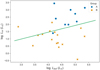 |
Fig. 4 Bolometric luminosity (L⊙) vs. outflow power Lm (L⊙) in logarithmic scale. |
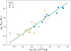 |
Fig. 5 Kinetic energy (1046 erg) vs. outflow mass (M⊙) in logarithmic scale. The Spearman ρ rank correlation coefficient is equal to 0.93 and the slope is equal to 0.69. |
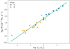 |
Fig. 6 Outflow power Lm (L⊙) vs. rate of matter expulsion Ṁ (10−4M⊙ yr−1) in logarithmic scale. The Spearman ρ rank correlation coefficient is equal to 0.97 and the slope is equal to 0.70. |
5.2 Evolutionary stage indicator L/M
The luminosity-to-mass ratio L/M can be used as an evolutionary stage indicator (e.g. Molinari et al. 2016; Elia et al. 2021; Urquhart et al. 2022). In the first stages of star formation the core is cold and actively accreting matter, so L/M ≤ 1. Eventually, the temperature and luminosity increase, while the mass remains virtually unchanged. This results in a value of L/M ≥ 1. It has been found that the more luminous sources in the Galaxy usually have L/M ≥ 10 (López-Sepulcre et al. 2011; Molinari et al. 2016). The sources in the sample studied here are in an advanced stage of the star-forming process as L/M has values ranging from 3 L⊙/M⊙ up to 177 L⊙/M⊙, with a mean of 58 L⊙/M⊙ and a median of 41 L⊙/M⊙ (see Table 2). Furthermore, we looked for correlations between L/M and the SiO outflow properties and found that they are not correlated. Other works have also failed to find such correlations (Liu et al. 2022, Liu et al 2021b; Maud et al. 2015). This strongly suggests that molecular outflows are present throughout the whole of the high-mass star formation process (Csengeri et al. 2016; Urquhart et al. 2022).
5.3 Cross-check between SiO and HCC+ wing detections
All of the sources that present wings in the HCO+ line also present SiO emission above 5σ. We compared these sources (Group A) with the rest of the clumps with SiO detections (Group B; see Table 6). Table 10 shows a statistical comparison of the spectral parameters, the outflow properties, and the evolutionary stage indicator L/M between these groups.
SiO spectral profiles with FWZP > 20 km s−1 are considered broad line widths due to high-velocity shocks (Duarte-Cabral et al. 2014; Zhu et al. 2020). We note that all the sources in both Groups A and Β exhibit broad line widths, with a minimum FWZP of 19.18 km s−1, a mean value of 47.15 km s−1, a median value of 44.86 km s−1, and a maximum of 92.12 km s−1. This means that all of the sources where SiO was detected have experienced recent outflow activity, which has manifested in high-velocity shocks, typically associated with collimated jets, and it is strong enough to produce SiO outflows (Csengeri et al. 2016; Li et al. 2019b; Liu et al. 2022). This confirms the sources in both Groups A and Β are protostellar (Zhu et al. 2020).
Furthermore, the SiO spectral profile of the sources in Group A is wider and more intense, indicating that the outflows in this group are more massive, faster and more energetic than those in Group Β (Schilke et al. 1997; Duarte-Cabral et al. 2014; Liu et al. 2022; see Table 10). Their mean outflow mass is higher than those in Group Β by a factor of 4.8, their mean momentum by a factor of 7, their mean kinetic energy by a factor of 14.7, their dynamic timescale by a factor of 0.58, their rate of matter expulsion by a factor of 8.7, their outflow force by a factor of 12, and their outflow power by a factor of 25.1. Sources in Group A are possibly more collimated too, as broad-width SiO detection is associated with them. Further studies of the spatial morphology of these outflows could confirm this trend.
Even though SiO outflow activity has been found to decrease and become less collimated over time (Arce et al. 2007; Sakai et al. 2010; López-Sepulcre et al. 2011), results show that sources in Groups A and Β are virtually at the same stage of evolution because their evolutionary stage indicator L/M have similar values. Table 10 shows that the evolutionary stage indicator L/M has a mean value of 40 (L⊙/M⊙) and 47 (L⊙/M⊙), and a median of 32 (L⊙/M⊙) and 29 (L⊙/M⊙) for Groups A and B, respectively. Thus, sources in Groups A and Β are most likely equally evolved, even within the protostellar phase (Motte et al. 2018). The fact that sources in Group A have more intense and massive SiO outflows, but both groups are at the same evolutionary stage, suggests that the presence of wings in the HCO+ spectral profile could help identify sources with stronger SiO outflows. Therefore, checking for wings in the HCO+ line could help identify more massive and active MSF regions in samples of similarly evolved sources. Alternatively, since HCO+ emission is associated with old outflow activity (Li et al. 2019a), sources in Group Β might have just recently started exhibiting strong outflow activity, thus allowing SiO outflows to be detected, and are too new to produce wings in the HCO+ spectral profile. Meanwhile, sources in Group A might have started exhibiting outflow activity long enough ago for wings in the HCO+ spectral profile, a signal of old outflows, to form. In this scenario, SiO outflows detected from the sources in Group A have been active for a longer time, which might be a consequence of their high mass, power, and luminosity. Thus, checking for wings in the HCO+ line might also help identify sources whose outflows have been active for longer. Further research with larger samples and better resolution could provide insight into which of these two scenarios is more likely and significant.
6 Summary and conclusions
The aim of this work was to study shocked matter and SiO outflows in very massive, luminous, and powerful protostellar sources. We characterised them, searched for any evolutionary trends they might exhibit, associated the presence of shocked gas with outflow activity, and cross-checked SiO emission with other outflow signatures. We used single-dish APEX/SEPIA Band 5 observations of 32 of the brightest massive protostellar sources in the southern Galaxy. We studied their outflow activity using the SiO and HCO+ tracers, as well as their general clump properties with H13CO+ emission. The following is a summary of our main results and conclusions:
The SiO emission detection rate above 5σ is 78% (25 sources). All SiO detections have a broad line width due to high-velocity shocks, which confirms that these sources have evolved well into the protostellar phase. Furthermore, 28% of our sample (nine sources) show wings in the HCO+ spectral profile.
We calculated the dynamical properties of the SiO outflows. Results show they are very massive, fast, and energetic. The outflow mass has a minimum value of 3 M⊙, a median of 10 M⊙, a mean of 30 M⊙, and a maximum value of 116 M⊙. The outflow momentum has a minimum value of 50 M⊙ km s−1, a median of 271 M⊙ km s−1, a mean of 922 M⊙ km s−1, and a maximum value of 4812 M⊙ km s−1. The kinetic energy of the outflow has a minimum value of 0.1 × 1046 erg, a median of 4 × 1046 erg, a mean of 27 × 1046 erg, and a maximum value of 183 × 1046 erg. The outflow power has a minimum value of 1.24 × 10⁻³Mo km s−1 yr−1, a median of 14.24 × 10⁻³M⊙ km s−1 yr−1, a mean of 102.25 × 10⁻³M⊙ km s−1 yr−1, and a maximum value of 884.85 × 10⁻³M⊙ km s−1 yr−1.
We found three positive linear correlations involving SiO outflows properties: a weak one between the bolometric luminosity and outflow power (Fig. 4), a strong one between the outflow power and the rate of matter expulsion (Fig. 6), and another strong one between the kinetic energy and outflow mass (Fig. 5). They are all positive correlations. The second and third have very low dispersion, but the second has high dispersion. These correlations suggest that the more energetic the outflow, the more material it is able to mobilise.
We did not find any correlations between the evolutionary stage indicator L/M and SiO outflow properties. This agrees with the idea that molecular outflows are a ubiquitous phenomenon throughout the process of high-mass star formation.
We performed a cross-check between SiO detection and the presence of wings in the HCO+ line. Sources in Group A (sources that present both features; see Table 6) have more massive, faster, more energetic, and more collimated SiO outflows than sources in Group B (sources that only exhibit SiO emission). The sources in both groups are at an advanced stage of evolution in the high-mass star formation process, and there is no clear evolutionary difference between them. Thus, since SiO emission is such a good tracer of outflow activity, checking for wings in the HCO+ line could help identify more massive and active MSF regions in samples of similarly evolved sources. Alternatively, checking for wings in the HCO+ line might help identify sources whose outflows have been active for longer, since HCO+ traces old outflow activity, whilst SiO traces recent and active outflows.
Our findings show the potential for further studies of sources at an advanced stage of evolution (L/M > 10) and their molecular outflows.
Statistics of the spectral parameters and outflow properties of sources from Groups A and B.
Acknowledgements
We thank the anonymous referee for their helpful and insightful comments. This publication is based on data acquired with the Atacama Pathfinder Experiment (APEX) under programme ID C-0102.F-9703B-2018 and C-0104.F-9702B-2019. APEX is a collaboration between the MaxPlanck-Institut fur Radioastronomie, the European Southern Observatory, and the Onsala Space Observatory. M.M. acknowledges support from ANID, Pro-grama de Astronomia - Fondo ALMA-CONICYT, project 3119AS0001. L.B. and R.F. gratefully acknowledge support by the ANID BASAL projects ACE210002 and FB210003, FONDEFID21I10359 and FONDECYT1221662. E.M. acknowledges support under the grant “Maria Zambrano” from the UHU funded by the Spanish Ministry of Universities and the “European Union NextGenerationEU”.
Appendix A Treatment of saturated sources
There are four sources in our sample with saturated observations (flagged with a ♦ in Tables 1 and 2): HC02, HC04, HC16, and HC20. Their dust mass Md was estimated at 500 (e.g. Merello et al. 2013; Motte et al. 2007),
 (A.1)
(A.1)
where D is the distance to the source, Fv is the flux density obtained from the Hi-GAL catalogue Elia et al. (2021), κν is the opacity, and Bv(Td) is Planck’s function at frequency ν = 599.585 GHz. The dust temperature Td was set to 25 K. The opacity κ500 for dense clumps with typical conditions has a value of 5.04 cm2 g−1 at 500 μm (Ossenkopf & Henning 1994).
The bolometric luminosity Lbo1 was calculated using the flux density at 70 obtained from the Hi-GAL catalogue, which has been found to be a good estimator for the total luminosity of protostellar objects when using the following empirical relation (Elia et al. 2017):
 (A.2)
(A.2)
Appendix B Distances
The distances used for the selection of the sources Dsel are the kinematic distances from Reid et al. (2009) using the local standard of rest velocity VLSR taken from Bronfman et al. (1996). Once the selection was made, the distances to the sources were corrected, as seen in Table B.1. The distance measured through trigonometric parallax from Reid et al. (2019) was used for the sources that have it. For the sources that do not have a distance calculated with parallax, the kinematic distances from Reid et al. (2014) were used instead. This left us with distances with the least possible uncertainty. These corrected distances were the ones used in the calculation of the properties of the sources.
Distances to the sources in the studied sample.
Appendix C Notes on particular sources
Some of the sources in our sample were found to be of particular interest because the intensity of their SiO outflows stands out from the rest (peak > 0.7 K). They are all of potential interest for future work. A brief description of the studies that have been carried out on these sources is provided here.
C.1 HC02: HIGALBM5.8856-0.3920, IRAS 17574-2403
This source (see Fig. 3) presents a particularly intense outflow. Although it is not the most massive, it has the maximum rate of matter expulsion calculated here. In addition, its spectral profiles shown in Fig. 3 suggest that there is a second cloud at 15.7 km s−1, and absorption at ~ 20 km s−1. It has been extensively studied since its discovery (Acord et al. 1997). Zahorecz et al. (2017) observed this source with APEX in the Band 5 and found that it does not present D2CO emission, suggesting that it is past the early stages of evolution. It was mapped at 12 mm and 7 mm by Nicholas et al. (2011a) and Nicholas et al. (2011b), respectively, and its [OI] spectra were resolved by Leurini et al. (2015). Its magnetic fields were studied by Tang et al. (2009) and Fernández-López et al. (2021). Su et al. (2009) reported a dense and hot-molecular cocoon in the environment of the source. Furthermore, its outflow has been extensively studied. The outflow of this source was mapped in the SiO(5-4) line by Sollins et al. (2004), traced in the SiO(8-7) line by Klaassen & Wilson (2007), and Zapata et al. (2019) found indications that it is an explosive multi-polar outflow. This was confirmed in Zapata et al. (2020), where a graph and an animation modelling the source are presented, clearly showing the multiple lobes.
C.2 HC08: HIGALBM301.1365-0.2259, IRAS 12326-6245
This source (see Fig. D.7) presents the most intense (Tpeak = 1.57 K) SiO emission in our sample and the most massive outflow (Mout = 116 M⊙). There are multiple infrared and radio sources deeply embedded in this clump (Henning et al. 2000; Murphy et al. 2010), and it presents one of the strongest molecular outflows in the southern sky (Araya et al. 2005). This suggests it is already at an advanced stage of evolution (Dedes et al. 2011). Finally, Duronea et al. (2021) present a study of the IR bubble S169 associated with this source, and conclude that star formation is actively taking place.
C.3 HC17: HIGALBM331.2786-0.1883, IRAS 16076-5134
This source presents one of the strongest outflows in our sample, which is clearly seen in both its HCO+ and SiO lines (see Fig. D.16). Its HCO+ line presents significant absorption and the SiO profile is one of the widest in our sample (FWZP = 52.26 km s−1). It has been an object of interest in numerous studies. Zinchenko et al. (2000) present C18O and HNCO observations and find that HNCO emission is most likely related to shocks of matter, similar to SiO emission. They detected HNCO emission in this source. Lee et al. (2001) and Lee et al. (2002) reported shock-excited H2 emission in addition to an outflow powered by a deeply embedded object in the former. Furthermore, De Buizer et al. (2009) present single-dish SiO(6-5) observations and evidence of outflow, and Baug et al. (2020) present images of the CO outflow observed with ALMA.
C.4 HC20: HIGALBM333.1246-0.4244, IRAS 16172-5028
The SiO intensity and the clear asymmetry of the spectral lines of this source make it particularly interesting. As is clear in Fig. D.19, its HCO+ line experiences more absorption on the blue side than on the red side. The H13CO+ even shows a wing on the red side, indicating that the outflow is particularly intense. The SiO line has a particular profile: its intensity decreases at the same velocity as the HCO+ absorption and the H13CO+ wing. This suggests that there might be a second colder cloud at around 50 km s−1. Rojas-García et al. (2022) map this source at 216.968 GHz and also report the possibility of a second source nearby. They also present a chemical profile of this source, where several COMs and SiO are detected. This source was also studied by Lo et al. (2007), where strong SiO and water maser emissions were detected. Lo et al. (2014) present a [CI] mapping of the source. Moreover, Figuerêdo et al. (2005) show that this source contains an embedded OB star cluster at very early evolutionary stages, and the presence of infall was confirmed by Wiles et al. (2016).
C.5 HC21: HIGALBM335.5848-0.2894, IRAS 16272-4837
This source presents one of the most intense (97.0 km s−1) and wide (57.41 km s−1) SiO profiles in the sample, as clearly seen in Fig. D.20. The studies done on this source include the discovery of water emission towards this source (van der Tak, F. F. S. et al. 2019), which has also been used as an evolutionary indicator because it can only be detected when the inner hot gas has reached a temperature of at least 300 K (van der Tak 2004). Emission of HNCO, another shock tracer, was found by Yu et al. (2018). Moreover, Garay et al. (2002) suggest that there is a young massive protostar embedded in this clump and it is still undergoing an intense accretion phase. This corresponds well with our findings and further suggests that it is a HMC. Finally, ALMA observations of this source have been presented by Olguin et al. (2021), where there is evidence of infall and rotation motions.
C.6 HC27: HIGALBM345.0035-0.2239, IRAS 17016-4124
This source presents a very wide (68.36 km s−1) and intense (1.02 K) SiO emission (see Fig. D.26). In addition, its HCO+ profile presents significant self-absorption and absorption. These characteristics make it a particularly interesting source. Several studies have conducted observations towards this source. Zinchenko et al. (2000) present C18O and HNCO emission observations, where it was found that high-velocity gas enhances the abundance of HNCO. Furthermore, mid-infrared observations are presented by Morales et al. (2009), and Testi et al. (1998) present H2O maser emission detection. Krishnan et al. (2013) and Voronkov et al. (2014) have found methanol maser emission as well. This source has been mapped with Large APEX BOlometer CAmera (LABOCA) at APEX by Gómez et al. (2014). Finally, Yu & Wang (2015) present MALT90 (Millimetre Astronomy Legacy Team 90 GHz) observations of the N2H+, H13CO+, HCO+, HNC, C2H HC3N and SiO spectral lines, and conclude that the sources in their sample are associated with dense clumps and recent outflow activity.
Appendix D Spectral profiles at the SiO(4-3), H13CO+(2-1), and HCO+(2-1) lines
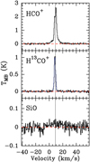 |
Fig. D.1 Spectral profiles for source HC01, Group C. The red dotted line is at FWZP, and the blue line in the H13CO+ panel shows the Gaussian fit. |
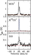 |
Fig. D.2 Spectral profiles for source HC03, Group B. The red dotted line is at FWZP, and the blue line in the H13CO+ panel shows the Gaussian fit. |
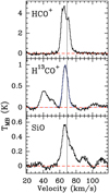 |
Fig. D.3 Spectral profiles for source HC04, Group B. The red dotted line is at FWZP, and the blue line in the H13CO+ panel shows the Gaussian fit. |
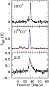 |
Fig. D.4 Spectral profiles for source HC05, Group B. The red dotted line is at FWZP, and the blue line in the H13CO+ panel shows the Gaussian fit. |
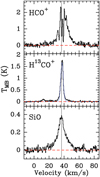 |
Fig. D.5 Spectral profiles for source HC06, Group B. The red dotted line is at FWZP, and the blue line in the H13CO+ panel shows the Gaussian fit. |
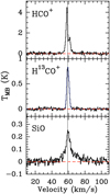 |
Fig. D.6 Spectral profiles for source HC07, Group B. The red dotted line is at FWZP, and the blue line in the H13CO+ panel shows the Gaussian fit. |
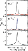 |
Fig. D.7 Spectral profiles for source HC08, Group A. The red dotted line is at FWZP, and the blue line in the H13CO+ panel shows the Gaussian fit. |
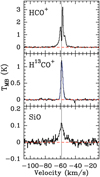 |
Fig. D.8 Spectral profiles for source HC09, Group B. The red dotted line is at FWZP, and the blue line in the H13CO+ panel shows the Gaussian fit. |
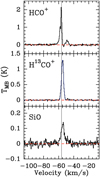 |
Fig. D.9 Spectral profiles for source HC10, Group B. The red dotted line is at FWZP, and the blue line in the H13CO+ panel shows the Gaussian fit. |
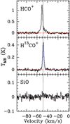 |
Fig. D.10 Spectral profiles for source HC11, Group C. The red dotted line is at FWZP, and the blue line in the H13CO+ panel shows the Gaussian fit. |
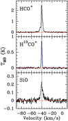 |
Fig. D.11 Spectral profiles for source HC12, Group B. The red dotted line is at FWZP, and the blue line in the H13CO+ panel shows the Gaussian fit. |
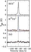 |
Fig. D.12 Spectral profiles for source HC13, Group C. The red dotted line is at FWZP, and the blue line in the H13CO+ panel shows the Gaussian fit. |
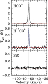 |
Fig. D.13 Spectral profiles for source HC14, Group C. The red dotted line is at FWZP, and the blue line in the H13CO+ panel shows the Gaussian fit. |
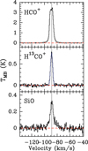 |
Fig. D.14 Spectral profiles for source HC15, Group B. The red dotted line is at FWZP, and the blue line in the H13CO+ panel shows the Gaussian fit. |
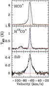 |
Fig. D.15 Spectral profiles for source HC16, Group A. The red dotted line is at FWZP, and the blue line in the H13CO+ panel shows the Gaussian fit. |
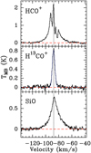 |
Fig. D.16 Spectral profiles for source HC17, Group A. The red dotted line is at FWZP, and the blue line in the H13CO+ panel shows the Gaussian fit. |
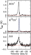 |
Fig. D.17 Spectral profiles for source HC18, Group A. The red dotted line is at FWZP, and the blue line in the H13CO+ panel shows the Gaussian fit. |
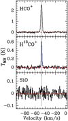 |
Fig. D.18 Spectral profiles for source HC19, Group C. The red dotted line is at FWZP, and the blue line in the H13CO+ panel shows the Gaussian fit. |
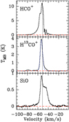 |
Fig. D.19 Spectral profiles for source HC20, Group A. The red dotted line is at FWZP, and the blue line in the H13CO+ panel shows the Gaussian fit. |
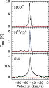 |
Fig. D.20 Spectral profiles for source HC21, Group A. The red dotted line is at FWZP, and the blue line in the H13CO+ panel shows the Gaussian fit. |
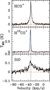 |
Fig. D.21 Spectral profiles for source HC22, Group A. The red dotted line is at FWZP, and the blue line in the H13CO+ panel shows the Gaussian fit. |
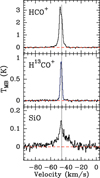 |
Fig. D.22 Spectral profiles for source HC23, Group B. The red dotted line is at FWZP, and the blue line in the H13CO+ panel shows the Gaussian fit. |
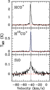 |
Fig. D.23 Spectral profiles for source HC24, Group B. The red dotted line is at FWZP, and the blue line in the H13CO+ panel shows the Gaussian fit. |
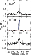 |
Fig. D.24 Spectral profiles for source HC25, Group B. The red dotted line is at FWZP, and the blue line in the H13CO+ panel shows the Gaussian fit. |
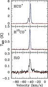 |
Fig. D.25 Spectral profiles for source HC26, Group B. The red dotted line is at FWZP, and the blue line in the H13CO+ panel shows the Gaussian fit. |
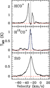 |
Fig. D.26 Spectral profiles for source HC27, Group B. The red dotted line is at FWZP, and the blue line in the H13CO+ panel shows the Gaussian fit. |
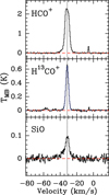 |
Fig. D.27 Spectral profiles for source HC28, Group B. The red dotted line is at FWZP, and the blue line in the H13CO+ panel shows the Gaussian fit. |
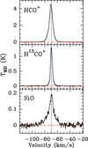 |
Fig. D.28 Spectral profiles for source HC29, Group A. The red dotted line is at FWZP, and the blue line in the H13CO+ panel shows the Gaussian fit. |
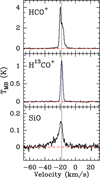 |
Fig. D.29 Spectral profiles for source HC30, Group B. The red dotted line is at FWZP, and the blue line in the H13CO+ panel shows the Gaussian fit. |
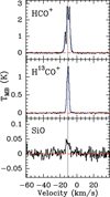 |
Fig. D.30 Spectral profiles for source HC31, Group C. The red dotted line is at FWZP, and the blue line in the H13CO+ panel shows the Gaussian fit. |
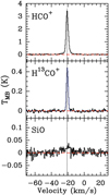 |
Fig. D.31 Spectral profiles for source HC32, Group C. The red dotted line is at FWZP, and the blue line in the H13CO+ panel shows the Gaussian fit. |
References
- Acord, J. M., Walmsley, C. M., & Churchwell, E. 1997, ApJ, 475, 693 [NASA ADS] [CrossRef] [Google Scholar]
- Araya, E., Hofner, P., Kurtz, S., Bronfman, L., & DeDeo, S. 2005, ApJS, 157, 279 [NASA ADS] [CrossRef] [Google Scholar]
- Arce, H. G., Shepherd, D., Gueth, F., et al. 2007, in Protostars and Planets V, eds. B. Reipurth, D. Jewitt, & K. Keil (Tucson: University of Arizona Press), 245 [Google Scholar]
- Bally, J. 2016, ARA&A, 54, 491 [Google Scholar]
- Baug, T., Wang, K., Liu, T., et al. 2020, ApJ, 890, 44 [NASA ADS] [CrossRef] [Google Scholar]
- Belitsky, V., Lapkin, I., Fredrixon, M., et al. 2018, A&A, 612, A23 [NASA ADS] [CrossRef] [EDP Sciences] [Google Scholar]
- Beuther, H., Schilke, P., Menten, K. M., et al. 2002, ASP Conf. Ser., 267, 341 [NASA ADS] [Google Scholar]
- Blake, G. A., Sutton, E. C., Masson, C. R., & Phillips, T. G. 1987, ApJ, 315, 621 [Google Scholar]
- Bronfman, L., Nyman, L. A., & May, J. 1996, A&AS, 115, 81 [Google Scholar]
- Butler, M. J., & Tan, J. C. 2012, ApJ, 754, 5 [Google Scholar]
- Codella, C., Bachiller, R., & Reipurth, B. 1999, A&A, 343, 585 [NASA ADS] [Google Scholar]
- Csengeri, T., Leurini, S., Wyrowski, F., et al. 2016, A&A, 586, A149 [NASA ADS] [CrossRef] [EDP Sciences] [Google Scholar]
- De Buizer, J. M., Redman, R. O., Longmore, S. N., Caswell, J., & Feldman, P. A. 2009, A&A, 493, 127 [NASA ADS] [CrossRef] [EDP Sciences] [Google Scholar]
- Dedes, C., Leurini, S., Wyrowski, F., et al. 2011, A&A, 526, A59 [NASA ADS] [CrossRef] [EDP Sciences] [Google Scholar]
- De Simone, M., Codella, C., Ceccarelli, C., et al. 2022, MNRAS, 512, 5214 [CrossRef] [Google Scholar]
- Duarte-Cabral, A., Bontemps, S., Motte, F., et al. 2014, A&A, 570, A1 [NASA ADS] [CrossRef] [EDP Sciences] [Google Scholar]
- Duronea, N. U., Cichowolski, S., Bronfman, L., et al. 2021, A&A, 646, A103 [NASA ADS] [CrossRef] [EDP Sciences] [Google Scholar]
- Dutrey, A., Guilloteau, S., & Guelin, M. 1997, A&A, 317, L55 [NASA ADS] [Google Scholar]
- Elia, D., Molinari, S., Fukui, Y., et al. 2013, ApJ, 772, 45 [NASA ADS] [CrossRef] [Google Scholar]
- Elia, D., Molinari, S., Schisano, E., et al. 2017, MNRAS, 471, 100 [NASA ADS] [CrossRef] [Google Scholar]
- Elia, D., Merello, M., Molinari, S., et al. 2021, MNRAS, 504, 2742 [NASA ADS] [CrossRef] [Google Scholar]
- Fernández-López, M., Sanhueza, P., Zapata, L. A., et al. 2021, ApJ, 913, 29 [CrossRef] [Google Scholar]
- Figuerêdo, E., Blum, R. D., Damineli, A., & Conti, P. S. 2005, AJ, 129, 1523 [CrossRef] [Google Scholar]
- Garay, G., Brooks, K. J., Mardones, D., Norris, R. P., & Burton, M. G. 2002, ApJ, 579, 678 [NASA ADS] [CrossRef] [Google Scholar]
- Garay, G., Mardones, D., Bronfman, L., et al. 2010, ApJ, 710, 567 [NASA ADS] [CrossRef] [Google Scholar]
- Garden, R. P., Hayashi, M., Gatley, I., Hasegawa, T., & Kaifu, N. 1991, ApJ, 374, 540 [NASA ADS] [CrossRef] [Google Scholar]
- Gómez, L., Wyrowski, F., Schuller, F., Menten, K. M., & Ballesteros-Paredes, J. 2014, A&A, 561, A148 [NASA ADS] [CrossRef] [EDP Sciences] [Google Scholar]
- Gusdorf, A., Cabrit, S., Flower, D. R., & Pineau des Forêts, G. 2008, A&A, 482, 809 [NASA ADS] [CrossRef] [EDP Sciences] [Google Scholar]
- He, Y.-X., Henkel, C., Zhou, J.-J., et al. 2021, ApJS, 253, 2 [NASA ADS] [CrossRef] [Google Scholar]
- Henning, T., Lapinov, A., Schreyer, K., Stecklum, B., & Zinchenko, I. 2000, A&A, 364, 613 [NASA ADS] [Google Scholar]
- Jiao, W., Wang, K., Pillai, T. G. S., et al. 2023, ApJ, 945, 81 [NASA ADS] [CrossRef] [Google Scholar]
- Klaassen, P. D., & Wilson, C. D. 2007, ApJ, 663, 1092 [NASA ADS] [CrossRef] [Google Scholar]
- Krishnan, V., Ellingsen, S. P., Voronkov, M. A., & Breen, S. L. 2013, MNRAS, 433, 3346 [NASA ADS] [CrossRef] [Google Scholar]
- Lee, J.-K., Walsh, A., Burton, M., & Ashley, M. 2001, MNRAS, 324, 1102 [NASA ADS] [CrossRef] [Google Scholar]
- Lee, J. K., Walsh, A. J., & Burton, M. G. 2002, IAU Symp., 206, 175 [NASA ADS] [Google Scholar]
- Leurini, S., Codella, C., López-Sepulcre, A., et al. 2014, A&A, 570, A49 [NASA ADS] [CrossRef] [EDP Sciences] [Google Scholar]
- Leurini, S., Wyrowski, F., Wiesemeyer, H., et al. 2015, A&A, 584, A70 [NASA ADS] [CrossRef] [EDP Sciences] [Google Scholar]
- Li, Q., Zhou, J., Esimbek, J., et al. 2019a, MNRAS, 488, 4638 [NASA ADS] [CrossRef] [Google Scholar]
- Li, S., Wang, J., Fang, M., et al. 2019b, ApJ, 878, 29 [NASA ADS] [CrossRef] [Google Scholar]
- Li, S., Zhang, Q., Pillai, T., et al. 2019c, ApJ, 886, 130 [Google Scholar]
- Li, S., Sanhueza, P., Zhang, Q., et al. 2020, ApJ, 903, 119 [Google Scholar]
- Liu, H.-L., Sanhueza, P., Liu, T., et al. 2020, ApJ, 901, 31 [NASA ADS] [CrossRef] [Google Scholar]
- Liu, M., Tan, J. C., Marvil, J., et al. 2021a, ApJ, 921, 96 [NASA ADS] [CrossRef] [Google Scholar]
- Liu, D.J., D.-J., Xu, Y., Li, Y.-J., et al. 2021b, ApJS, 253, 15 [NASA ADS] [CrossRef] [Google Scholar]
- Liu, R., Liu, T., Chen, G., et al. 2022, MNRAS, 511, 3618 [CrossRef] [Google Scholar]
- Lo, N., Cunningham, M., Bains, I., Burton, M. G., & Garay, G. 2007, MNRAS, 381, L30 [NASA ADS] [Google Scholar]
- Lo, N., Cunningham, M. R., Jones, P. A., et al. 2014, ApJ, 797, L17 [NASA ADS] [CrossRef] [Google Scholar]
- López-Sepulcre, A., Walmsley, C. M., Cesaroni, R., et al. 2011, A&A, 526, L2 [NASA ADS] [CrossRef] [EDP Sciences] [Google Scholar]
- López-Sepulcre, A., Watanabe, Y., Sakai, N., et al. 2016, ApJ, 822, 85 [CrossRef] [Google Scholar]
- Martin-Pintado, J., Bachiller, R., & Fuente, A. 1992, A&A, 254, 315 [NASA ADS] [Google Scholar]
- Maud, L. T., Moore, T. J. T., Lumsden, S. L., et al. 2015, MNRAS, 453, 645 [Google Scholar]
- Merello, M., Bronfman, L., Garay, G., et al. 2013, ApJ, 774, 38 [NASA ADS] [CrossRef] [Google Scholar]
- Merello, M., Molinari, S., Rygl, K. L. J., et al. 2018, MNRAS, 483, 5355 [Google Scholar]
- Mladenović, M. 2017, AIP, 147, 24 [Google Scholar]
- Molinari, S., Merello, M., Elia, D., et al. 2016, ApJ, 826, L8 [Google Scholar]
- Morales, E. F. E., Mardones, D., Garay, G., Brooks, K. J., & Pineda, J. E. 2009, ApJ, 698, 488 [NASA ADS] [CrossRef] [Google Scholar]
- Motte, F., Bontemps, S., Schilke, P., et al. 2007, A&A, 476, 1243 [NASA ADS] [CrossRef] [EDP Sciences] [Google Scholar]
- Motte, F., Zavagno, A., Bontemps, S., et al. 2010, A&A, 518, L77 [CrossRef] [EDP Sciences] [Google Scholar]
- Motte, F., Bontemps, S., & Louvet, F. 2018, ARA&A, 56, 41 [NASA ADS] [CrossRef] [Google Scholar]
- Murphy, T., Cohen, M., Ekers, R. D., et al. 2010, MNRAS, 405, 1560 [Google Scholar]
- Myers, P. C., Mardones, D., Tafalla, M., Williams, J. P., & Wilner, D. J. 1996, ApJ, 465, L133 [NASA ADS] [CrossRef] [Google Scholar]
- Nicholas, B., Rowell, G., Burton, M. G., et al. 2011a, MNRAS, 411, 1367 [CrossRef] [Google Scholar]
- Nicholas, B. P., Rowell, G., Burton, M. G., et al. 2011b, MNRAS, 419, 251 [Google Scholar]
- Olguin, F. A., Sanhueza, P., Guzmán, A. E., et al. 2021, ApJ, 909, 199 [NASA ADS] [CrossRef] [Google Scholar]
- Ossenkopf, V., & Henning, T. 1994, A&A, 291, 943 [NASA ADS] [Google Scholar]
- Pedregosa, F., Varoquaux, G., Gramfort, A., et al. 2011 J. Mach. Learn. Res., 12, 2825 [Google Scholar]
- Rawlings, J. M. C., Redman, M. P., Keto, E., & Williams, D. A. 2004, MNRAS, 351, 1054 [Google Scholar]
- Reid, M. J., Menten, K. M., Zheng, X. W., et al. 2009, ApJ, 700, 137 [CrossRef] [Google Scholar]
- Reid, M. J., Menten, K. M., Brunthaler, A., et al. 2014, ApJ, 783, 130 [Google Scholar]
- Reid, M. J., Menten, K. M., Brunthaler, A., et al. 2019, ApJ, 885, 131 [Google Scholar]
- Rojas-García, O. S., Gómez-Ruiz, A. I., Palau, A., et al. 2022, ApJS, 262, 13 [CrossRef] [Google Scholar]
- Sakai, T., Sakai, N., Hirota, T., & Yamamoto, S. 2010, ApJ, 714, 1658 [NASA ADS] [CrossRef] [Google Scholar]
- Sanhueza, P., Jackson, J. M., Foster, J. B., et al. 2012, ApJ, 756, 60 [Google Scholar]
- Schilke, P., Walmsley, C. M., Pineau des Forets, G., & Flower, D. R. 1997, A&A, 321, 293 [NASA ADS] [Google Scholar]
- Shirley, Y. L. 2015, PASP, 127, 299 [Google Scholar]
- Sollins, P. K., Hunter, T. R., Battat, J., et al. 2004, ApJ, 616, L35 [NASA ADS] [CrossRef] [Google Scholar]
- Su, Y.-N., Liu, S.-Y., Wang, K.-S., Chen, Y.-H., & Chen, H.-R. 2009, ApJ, 704, L5 [NASA ADS] [CrossRef] [Google Scholar]
- Tang, Y.-W., Ho, P. T. P., Girart, J. M., et al. 2009, ApJ, 695, 1399 [Google Scholar]
- Testi, L., Felli, M., Persi, P., & Roth, M. 1998, A&AS, 129, 495 [NASA ADS] [CrossRef] [EDP Sciences] [Google Scholar]
- Urquhart, J. S., Wells, M. R. A., Pillai, T., et al. 2022, MNRAS, 510, 3389 [NASA ADS] [CrossRef] [Google Scholar]
- van der Tak, F. F. S. 2004, in Star Formation at High Angular Resolution, eds. M. G. Burton, R. Jayawardhana, & T. L. Bourke (Amsterdam: Elsevier), 221, 59 [NASA ADS] [Google Scholar]
- van der Tak, F. F. S., Shipman, R. F., Jacq, T., et al. 2019, A&A, 625, A103 [NASA ADS] [CrossRef] [EDP Sciences] [Google Scholar]
- Voronkov, M. A., Caswell, J. L., Ellingsen, S. P., Green, J. A., & Breen, S. L. 2014, MNRAS, 439, 2584 [NASA ADS] [CrossRef] [Google Scholar]
- Widmann, F., Beuther, H., Schilke, P., & Stanke, T. 2016, A&A, 589, A29 [NASA ADS] [CrossRef] [EDP Sciences] [Google Scholar]
- Wiles, B., Lo, N., Redman, M. P., et al. 2016, MNRAS, 458, 3429 [NASA ADS] [CrossRef] [Google Scholar]
- Wu, Y., Wei, Y., Zhao, M., et al. 2004, A&A, 426, 503 [NASA ADS] [CrossRef] [EDP Sciences] [Google Scholar]
- Wu, Y., Zhu, M., Wei, Y., et al. 2005, ApJ, 628, L57 [NASA ADS] [CrossRef] [Google Scholar]
- Yang, A. Y., Urquhart, J. S., Wyrowski, F., et al. 2022, A&A, 658, A160 [NASA ADS] [CrossRef] [EDP Sciences] [Google Scholar]
- Yu, N., & Wang, J.-J. 2015, MNRAS, 451, 2507 [NASA ADS] [CrossRef] [Google Scholar]
- Yu, N.-P., Xu, J.-L., & Wang, J.-J. 2018, RAA, 18, 015 [NASA ADS] [Google Scholar]
- Zahorecz, S., Jimenez-Serra, I., Testi, L., et al. 2017, A&A, 602, L3 [NASA ADS] [CrossRef] [EDP Sciences] [Google Scholar]
- Zapata, L. A., Ho, P. T. P., Guzmán Ccolque, E., et al. 2019, MNRAS, 486, L15 [NASA ADS] [Google Scholar]
- Zapata, L. A., Ho, P. T. P., Fernández-López, M., et al. 2020, ApJ, 902, L47 [Google Scholar]
- Zhu, F.-Y., Wang, J.-Z., Liu, T., et al. 2020, MNRAS, 499, 6018 [NASA ADS] [CrossRef] [Google Scholar]
- Zinchenko, I., Henkel, C., & Mao, R. Q. 2000, A&A, 361, 1079 [NASA ADS] [Google Scholar]
- Ziurys, L. M., Friberg, P., & Irvine, W. M. 1989, ApJ, 343, 201 [NASA ADS] [CrossRef] [Google Scholar]
All Tables
Statistics of the spectral parameters and outflow properties of sources from Groups A and B.
All Figures
|
Fig. 1 Histogram of the luminosity-to-mass ratio L/M in logarithmic scale. The red and purple vertical lines denote the median (30 L⊙/M⊙) and the mean (45 L⊙/M⊙), respectively. Groups A, B, and C are defined in Table 6. |
| In the text | |
|
Fig. 2 Galactic distribution of the sources. The orange point corresponds to the Sun and the green point to the Galactic centre. The red crosses are the sources studied in this paper. The blue circles are centred on the Sun and the black circles on the Galactic centre. They indicate the 1, 5, and 10 kpc distances. |
| In the text | |
|
Fig. 3 Spectral profiles for source HC02, Group A. The red dotted line is at FWZP and the blue line in the H13CO+ panel shows the Gaussian fit. |
| In the text | |
|
Fig. 4 Bolometric luminosity (L⊙) vs. outflow power Lm (L⊙) in logarithmic scale. |
| In the text | |
|
Fig. 5 Kinetic energy (1046 erg) vs. outflow mass (M⊙) in logarithmic scale. The Spearman ρ rank correlation coefficient is equal to 0.93 and the slope is equal to 0.69. |
| In the text | |
|
Fig. 6 Outflow power Lm (L⊙) vs. rate of matter expulsion Ṁ (10−4M⊙ yr−1) in logarithmic scale. The Spearman ρ rank correlation coefficient is equal to 0.97 and the slope is equal to 0.70. |
| In the text | |
|
Fig. D.1 Spectral profiles for source HC01, Group C. The red dotted line is at FWZP, and the blue line in the H13CO+ panel shows the Gaussian fit. |
| In the text | |
|
Fig. D.2 Spectral profiles for source HC03, Group B. The red dotted line is at FWZP, and the blue line in the H13CO+ panel shows the Gaussian fit. |
| In the text | |
|
Fig. D.3 Spectral profiles for source HC04, Group B. The red dotted line is at FWZP, and the blue line in the H13CO+ panel shows the Gaussian fit. |
| In the text | |
|
Fig. D.4 Spectral profiles for source HC05, Group B. The red dotted line is at FWZP, and the blue line in the H13CO+ panel shows the Gaussian fit. |
| In the text | |
|
Fig. D.5 Spectral profiles for source HC06, Group B. The red dotted line is at FWZP, and the blue line in the H13CO+ panel shows the Gaussian fit. |
| In the text | |
|
Fig. D.6 Spectral profiles for source HC07, Group B. The red dotted line is at FWZP, and the blue line in the H13CO+ panel shows the Gaussian fit. |
| In the text | |
|
Fig. D.7 Spectral profiles for source HC08, Group A. The red dotted line is at FWZP, and the blue line in the H13CO+ panel shows the Gaussian fit. |
| In the text | |
|
Fig. D.8 Spectral profiles for source HC09, Group B. The red dotted line is at FWZP, and the blue line in the H13CO+ panel shows the Gaussian fit. |
| In the text | |
|
Fig. D.9 Spectral profiles for source HC10, Group B. The red dotted line is at FWZP, and the blue line in the H13CO+ panel shows the Gaussian fit. |
| In the text | |
|
Fig. D.10 Spectral profiles for source HC11, Group C. The red dotted line is at FWZP, and the blue line in the H13CO+ panel shows the Gaussian fit. |
| In the text | |
|
Fig. D.11 Spectral profiles for source HC12, Group B. The red dotted line is at FWZP, and the blue line in the H13CO+ panel shows the Gaussian fit. |
| In the text | |
|
Fig. D.12 Spectral profiles for source HC13, Group C. The red dotted line is at FWZP, and the blue line in the H13CO+ panel shows the Gaussian fit. |
| In the text | |
|
Fig. D.13 Spectral profiles for source HC14, Group C. The red dotted line is at FWZP, and the blue line in the H13CO+ panel shows the Gaussian fit. |
| In the text | |
|
Fig. D.14 Spectral profiles for source HC15, Group B. The red dotted line is at FWZP, and the blue line in the H13CO+ panel shows the Gaussian fit. |
| In the text | |
|
Fig. D.15 Spectral profiles for source HC16, Group A. The red dotted line is at FWZP, and the blue line in the H13CO+ panel shows the Gaussian fit. |
| In the text | |
|
Fig. D.16 Spectral profiles for source HC17, Group A. The red dotted line is at FWZP, and the blue line in the H13CO+ panel shows the Gaussian fit. |
| In the text | |
|
Fig. D.17 Spectral profiles for source HC18, Group A. The red dotted line is at FWZP, and the blue line in the H13CO+ panel shows the Gaussian fit. |
| In the text | |
|
Fig. D.18 Spectral profiles for source HC19, Group C. The red dotted line is at FWZP, and the blue line in the H13CO+ panel shows the Gaussian fit. |
| In the text | |
|
Fig. D.19 Spectral profiles for source HC20, Group A. The red dotted line is at FWZP, and the blue line in the H13CO+ panel shows the Gaussian fit. |
| In the text | |
|
Fig. D.20 Spectral profiles for source HC21, Group A. The red dotted line is at FWZP, and the blue line in the H13CO+ panel shows the Gaussian fit. |
| In the text | |
|
Fig. D.21 Spectral profiles for source HC22, Group A. The red dotted line is at FWZP, and the blue line in the H13CO+ panel shows the Gaussian fit. |
| In the text | |
|
Fig. D.22 Spectral profiles for source HC23, Group B. The red dotted line is at FWZP, and the blue line in the H13CO+ panel shows the Gaussian fit. |
| In the text | |
|
Fig. D.23 Spectral profiles for source HC24, Group B. The red dotted line is at FWZP, and the blue line in the H13CO+ panel shows the Gaussian fit. |
| In the text | |
|
Fig. D.24 Spectral profiles for source HC25, Group B. The red dotted line is at FWZP, and the blue line in the H13CO+ panel shows the Gaussian fit. |
| In the text | |
|
Fig. D.25 Spectral profiles for source HC26, Group B. The red dotted line is at FWZP, and the blue line in the H13CO+ panel shows the Gaussian fit. |
| In the text | |
|
Fig. D.26 Spectral profiles for source HC27, Group B. The red dotted line is at FWZP, and the blue line in the H13CO+ panel shows the Gaussian fit. |
| In the text | |
|
Fig. D.27 Spectral profiles for source HC28, Group B. The red dotted line is at FWZP, and the blue line in the H13CO+ panel shows the Gaussian fit. |
| In the text | |
|
Fig. D.28 Spectral profiles for source HC29, Group A. The red dotted line is at FWZP, and the blue line in the H13CO+ panel shows the Gaussian fit. |
| In the text | |
|
Fig. D.29 Spectral profiles for source HC30, Group B. The red dotted line is at FWZP, and the blue line in the H13CO+ panel shows the Gaussian fit. |
| In the text | |
|
Fig. D.30 Spectral profiles for source HC31, Group C. The red dotted line is at FWZP, and the blue line in the H13CO+ panel shows the Gaussian fit. |
| In the text | |
|
Fig. D.31 Spectral profiles for source HC32, Group C. The red dotted line is at FWZP, and the blue line in the H13CO+ panel shows the Gaussian fit. |
| In the text | |
Current usage metrics show cumulative count of Article Views (full-text article views including HTML views, PDF and ePub downloads, according to the available data) and Abstracts Views on Vision4Press platform.
Data correspond to usage on the plateform after 2015. The current usage metrics is available 48-96 hours after online publication and is updated daily on week days.
Initial download of the metrics may take a while.