| Issue |
A&A
Volume 677, September 2023
|
|
|---|---|---|
| Article Number | A151 | |
| Number of page(s) | 10 | |
| Section | Galactic structure, stellar clusters and populations | |
| DOI | https://doi.org/10.1051/0004-6361/202244286 | |
| Published online | 20 September 2023 | |
Observational constraints on the origin of the elements
V. NLTE abundance ratios of [Ni/Fe] in Galactic stars and enrichment by sub-Chandrasekhar mass supernovae
1
Max Planck Institute for Astronomy, Königstuhl 17, 69117 Heidelberg, Germany
e-mail: This email address is being protected from spambots. You need JavaScript enabled to view it.
2
Ruprecht Karl University of Heidelberg, Grabengasse 1, 69117 Heidelberg, Germany
3
Niels Bohr International Academy, Niels Bohr Institute, University of Copenhagen, Blegdamsvej 17, 2100 Copenhagen, Denmark
4
School of Science, University of New South Wales Canberra The Australian Defence Force Academy, 2600 Canberra, ACT, Australia
5
Department of Physics and Astronomy, University of Victoria, Victoria, V8P 5C2 BC, Canada
6
Konkoly Observatory, Research Centre for Astronomy and Earth Sciences, Eötvös Loránd Research Network (ELKH), Konkoly Thege Miklós út 15-17, 1121 Budapest, Hungary
Received:
16
June
2022
Accepted:
11
July
2023
Abstract
Aims. We constrain the role of different Type Ia supernova (SN Ia) channels in the chemical enrichment of the Galaxy by studying the abundances of nickel in Galactic stars. We investigated four different SN Ia sub-classes, including the classical single-degenerate near-Chandrasekhar mass (Mch) SN Ia, the fainter SN Iax systems associated with He accretion from the companion, as well as two sub-Chandrasekhar mass (sub-Mch) SN Ia channels. The latter include the double detonation of a white dwarf accreting helium-rich matter and violent white dwarf mergers.
Methods. The chemical abundances in Galactic stars were determined using Gaia eDR3 astrometry and photometry and high-resolution optical spectra. Non-local thermodynamic equilibrium (NLTE) models of Fe and Ni were used in the abundance analysis. We included new delay-time distributions arising from the different SN Ia channels in models of the Galactic chemical evolution, as well as recent yields for core-collapse supernovae and asymptotic giant branch stars. The data-model comparison was performed using a Markov chain Monte Carlo framework that allowed us to explore the entire parameter space allowed by the diversity of explosion mechanisms and the Galactic SN Ia rate, taking the uncertainties of the observed data into account.
Results. We show that NLTE effects have a non-negligible impact on the observed [Ni/Fe] ratios in the Galactic stars. The NLTE corrections to Ni abundances are not large, but strictly positive, lifting the [Ni/Fe] ratios by ∼ + 0.15 dex at [Fe/H] −2. We find that the distributions of [Ni/Fe] in LTE and in NLTE are very tight, with a scatter of ≲0.1 dex at all metallicities. This supports earlier work. In LTE, most stars have scaled solar Ni abundances, [Ni/Fe] ≈ 0, with a slight tendency for sub-solar [Ni/Fe] ratios at lower [Fe/H]. In NLTE, however, we find a mild anti-correlation between [Ni/Fe] and metallicity, and slightly elevated [Ni/Fe] ratios at [Fe/H] ≲ −1.0. The NLTE data can be explained by models of the Galactic chemical evolution that are calculated with a substantial fraction, ∼75%, of sub-Mch SN Ia.
Key words: Galaxy: evolution / Galaxy: abundances / supernovae: general / supernovae: individual: SNe Ia / stars: abundances / nuclear reactions / nucleosynthesis / abundances
© The Authors 2023
 Open Access article, published by EDP Sciences, under the terms of the Creative Commons Attribution License (https://creativecommons.org/licenses/by/4.0), which permits unrestricted use, distribution, and reproduction in any medium, provided the original work is properly cited.
This article is published in open access under the Subscribe to Open model.
Open access funding provided by Max Planck Society.
1. Introduction
Type Ia supernovae (SN Ia) systems are of critical significance in modern astrophysics because they play a key role in extragalactic distance measurements (e.g. Phillips 1993; Riess et al. 1998, 2022), they contribute to chemical enrichment of stellar populations with Fe-peak elements (e.g. Timmes et al. 1995; Kobayashi et al. 2020), and they are sources of kinetic energy in galaxies. Recent studies (see e.g. Taubenberger 2017; Ruiter 2019) uncovered a great diversity of SN Ia types, associated with different explosions and progenitors of white dwarfs (WDs; Iben et al. 1987). These include canonical single-degenerate Chandrasekhar-mass (Mch) explosions caused by mass transfer onto a WD in a binary system, double-degenerate explosions associated with a violent merger of two WDs resulting in a prompt detonation (e.g. Pakmor et al. 2012), and scenarios in which He mass transfer from the companion leads to a surface He detonation triggering detonation in the CO core (e.g. Livne 1990; Fink et al. 2010; Shen et al. 2018; Goldstein & Kasen 2018). Additionally, head-on collisions in triples through the Lidov-Kozai mechanism are being explored (e.g. Antognini & Thompson 2016; Toonen et al. 2018).
However, constraining progenitor and explosion types by direct observations is difficult because their spectroscopic and photometric properties are similar (Branch 1998; Hillebrandt et al. 2013). Independent constraints can be obtained through studies of the integrated chemical enrichment of stellar populations that probe a range of ages and metallicities, that is, by combining observed abundances and models of Galactic chemical evolution (GCE; e.g. Timmes et al. 1995; Kobayashi et al. 2020). This approach is particularly valuable in the studies of properties of sub-Mch explosions (Seitenzahl et al. 2013a) because their associated integrated yields for Ni, Co, and Mn (e.g. Gronow et al. 2021; Boos et al. 2021) and delay times are in stark contrast to those of the classical Mch-SN Ia models (e.g. Ruiter et al. 2011; Goldstein & Kasen 2018). Recent studies of sub-Mch SNe fractions in the chemical evolution of the Milky Way and dwarf galaxies include Seitenzahl et al. (2013a), McWilliam et al. (2018), Kirby et al. (2019), Kobayashi et al. (2020), Eitner et al. (2020), de los Reyes et al. (2020), Lach et al. (2020), and Sanders et al. (2021). Except for Eitner et al. (2020) and McWilliam et al. (2018), most other studies relied either on local thermodynamic equilibrium (LTE) calculations of stellar photospheric abundances or on mixed LTE and NLTE estimates. They combined for instance NLTE measurements of Fe abundances with LTE estimates of Ni abundances (as in Sanders et al. 2021).
In this paper, we use the new data sets for [Ni/Fe] to study the role of sub-Mch SN Ia channels in the chemical enrichment of the Galaxy. The Ni abundances in NLTE are derived for the first time for the Galactic stars. Starting with a summary of the observational sample in Sect. 2, we provide details on the methods for deriving and modelling explosion channels as well as abundance tracks in Sect. 3. The results are then presented in Sect. 4 and discussed in the light of similar studies in Sect. 5. We close with conclusions and a future outlook in Sect. 6.
2. Observations and stellar parameters
2.1. Main stellar sample
We used public spectra obtained within the Gaia-ESO1 survey data (Gilmore et al. 2022; Randich et al. 2022). The Gaia-ESO survey was designed to comprehensively cover the Galactic disk, halo, and stellar clusters because one of the major science goals was to constrain the Galactic structure and evolution. The survey was executed on the Very Large Telescope (VLT) from 2013 to 2018. In this work, we use only the high-resolution R ∼ 47 000 spectra taken in the UVES 580 setting (λ 480 to 680 nm), and limit the analysis to data with a high signal-to-noise ratio (S/N) with S/N > ;60 for stars in the metallicity range above −0.7, which offers a reasonable trade-off between the number of stars over a representative metallicity range and the quality of the spectra.
The analysis of stellar parameters was carried out using the SAPP pipeline (Gent et al. 2022), which combines different types of observational information, including photometry, spectra, and parallaxes in the full Bayesian framework to provide estimates of Teff, log g, and [Fe/H]. The photometric magnitudes were adopted from the third data release (eDR3) of the Gaia catalogue (Gaia Collaboration 2021). The characteristic photometric errors range from 0.3 mmag to 6 mmag. Distances were adopted from the Bailer-Jones et al. (2021) catalogue. As recommended by these authors, we used their photo-geometric distances. To improve the quality of the abundance diagnostics, the Ni abundances were derived by a line-by-line analysis using the NLTE spectrum synthesis code TSFitPy (Gerber et al. 2023), along with grids of NLTE departure coefficients calculated with the MULTI2.3 code (Carlsson 1992) using updated NLTE atomic models of Fe (Semenova et al. 2020) and Ni (Bergemann et al. 2021; Magg et al. 2022). We note that in the latter model, the rates of transitions associated with charge-exchange reactions Ni+H were calculated using new quantum-mechanical data from Voronov et al. (2022). Figure 1 shows some examples of the observed spectra and the best fits for the Ni I 6086 Å and 6175 Å. Our final high-quality stellar sample consists of 264 stars with Ni abundances.
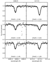 |
Fig. 1. Best-fit line profiles for two diagnostic lines of Ni for three representative stars at metallicities [Fe/H] = −0.34, −0.55, and −1.05. |
2.2. Additional samples
For comparison, we also included additional data sets. Specifically, we added the abundances from Bensby et al. (2014), who employed high-quality optical spectra taken from different facilities and with a resolving power in the range from R ∼ 47 000 to ∼110 000. The Fe abundances were corrected for NLTE effects based on the model atom and corrections from Bergemann et al. (2012) and Lind et al. (2012). We also corrected their LTE Ni abundances for NLTE using the direct line-to-line abundances for each individual star kindly provided to us by T. Bensby (priv. comm.). As a guidance, we present the NLTE Ni I corrections for three models representative of our stellar sample in Fig. 2. The NLTE effect on Ni abundances is rather modest but non-negligible at solar metallicity. However, especially at metallicities [Fe/H] ≲ −2, NLTE corrections for Ni increase and may reach +0.3 dex depending on the evolutionary stage of the star, which implies that NLTE abundances of Ni have to be used for a reliable chemical evolution modelling.
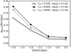 |
Fig. 2. Ni NLTE corrections as a function of metallicity for three representative stellar model atmospheres averaged over diagnostic lines of Ni I in the optical wavelength range. |
The Galactic [Fe/H]–[Ni/Fe] distributions from the combined sample are shown in Fig. 3. Our NLTE [Ni/Fe] results are higher than the LTE measurements, especially at low metallicity. This is fully expected given the NLTE effects in the diagnostic lines, which are primarily associated with over-excitation and over-ionisation in Ni I (Bergemann et al. 2014, 2021; Magg et al. 2022).
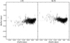 |
Fig. 3. Trends of [Ni/Fe] against metallicity [Fe/H], calculated in LTE (left) and NLTE (right). |
3. Methods
3.1. Chemical evolution model
We used the two-zone GCE model OMEGA+2 (Côté et al. 2017; Côté & Ritter 2018), which was chosen for its high flexibility regarding the treatment of chemical enrichment sources. The model is conceptually similar to other widely used analytical GCE models (e.g. Tinsley 1980; Matteucci & Greggio 1986; Matteucci 2004; Chiappini et al. 1997; Kobayashi et al. 2000; Gibson et al. 2003; Prantzos 2008; Yates et al. 2013; Rybizki et al. 2017; Weinberg et al. 2017). In what follows, we provide a compact summary of the basic ingredients of the model.
OMEGA+ supports in- and outflows, and its inner region represents a classical open-box, one-zone GCE model without the simplification of instantaneous recycling. The initial mass function is assumed to follow the Kroupa (2001) prescription, and the star formation rate (SFR) is computed using the Kennicutt–Schmidt law (Kennicutt 1998). The model furthermore relies on Heger & Woosley (2010) yields for Population III stars. The yields from asymptotic giant branch (AGB) and massive stars are discussed in Sect. 3.2, and the SN Ia yields are described in detail in Sect. 3.3. We modelled gas exchange with the circumgalactic medium using a classical double-exponential inflow rate that contains an initial burst of star formation with a decay scale of 0.68 Gyr and an additional period with a delay of 1 Gyr and duration of 7 Gyr, as proposed by Chiappini et al. (1997). The free parameters of the model are the star formation efficiency (SFE), the mass-loading factor, and the infall strength, and they were chosen such that the GCE model reproduces the present-day observables, including the SFR, gas mass, metallicity, and the total rate of SN Ia (Côté et al. 2019). In particular, for the specific model adopted in this work, we used logSFE ∼ −9.52 and a mass-loading factor of 0.5. The influence of the model parameters was investigated in our previous studies and is not repeated here. Specifically, the SFR, the mass-loading factor, inflows and outflows were discussed and explored in Côté et al. (2017, 2018). In the former study, this was done against observational constraints, and in the latter study, it was done within the scope of hydrodynamical simulations of galaxy formation.
3.2. Asymptotic giant branch and core-collapse explosions
We considered two sets of core-collapse (CC) SN yields that are commonly used in the literature, Nomoto et al. (2013) and Limongi & Chieffi (2018). We also investigated two widely used sets of AGB yields from Karakas (2010) and Cristallo et al. (2015).
The tables by Nomoto et al. (2013) include the yields from Nomoto et al. (2006), Kobayashi et al. (2006, 2011), and Tominaga et al. (2007), who considered masses between 13 and 40 M⊙ and metallicities Z between 0.001 and 0.05 (i.e. super-solar). The models hereby follow the mixing and fallback scheme by Umeda & Nomoto (2002). The yields were calibrated on observed spectra and light curves of CC SNe with respect to the progenitor mass, explosion energy, and 56Ni production of the models. In this paper, we did not include hypernovae because their role in the chemical evolution is still debated (see the discussion in Eitner et al. 2020). The massive star yields of Nomoto et al. (2013) were complemented with AGB yields from Cristallo et al. (2015).
Limongi & Chieffi (2018) focused on the analysis of the influence of rotational mixing on the evolution and explosion physics of massive stars. They presented a set of yields for stars in the mass range of 13 − 120 M⊙ and [Fe/H] = 0, −1, −2, −3. Mixing-fallback was included only for stars with mass below 25 M⊙. In their recommended model, they also assumed that stellar winds alone contribute to the chemical enrichment above this mass threshold due to a complete BH collapse. We adopted their models, which were computed using a metallicity-dependent average rotation velocity profile from Prantzos et al. (2018). Higher rotation velocities lead to continuous mixing during central He-burning, which introduces an important source of neutrons, thereby allowing for a more efficient production of heavy nuclei and effectively increasing Mn abundances at low metallicities. These massive star yields were supplemented by AGB star yields from Karakas (2010).
In Fig. 4 we compare the average yields from Nomoto et al. (2013, hereafter N13) and Limongi & Chieffi (2018, hereafter LC18). The yields of LC18 show significantly more Ni than Fe over the entire metallicity range compared to N13 yields. This difference has strong implications for the Galactic evolution of [Ni/Fe], and this is explored in detail in Sect. 4.2.
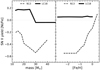 |
Fig. 4. Comparison of the integrated yields from CC SNe from Limongi & Chieffi (2018) and Nomoto et al. (2013). Top row: yields as a function of stellar mass, averaged over metallicity. Bottom panel: mass-averaged yields as a function of metallicity. |
3.3. Supernova Ia scenarios
We include here four common SN Ia scenarios: two with Mch WDs, and two with sub-Mch WD progenitors, as described in detail below. Different explosion mechanisms were assumed for different scenarios. For each of these models, the yield tables were adopted from the Heidelberg Supernova Model Archive (HESMA)3 (Kromer et al. 2017).
3.3.1. Yields
First, we considered the classical channel of a single-degenerate binary system that contains a primary near-Mch WD that receives H-rich material from a non-degenerate companion (the donor) via Roche-lobe overflow, and explodes in a delayed detonation (Khokhlov 1991). The yields adopted for events of this type were computed by Seitenzahl et al. (2013b), where the detailed hydrodynamics of the explosion process was modelled for different numbers and geometries of ignition conditions. We chose the same model as in Röpke et al. (2012), which consists of 100 partially overlapping ignition kernels in a symmetric orientation. The central density was assumed to be ∼2.9 × 10⁹ g cm−3, but Seitenzahl et al. (2013b) noted that the yields for slightly neutron-rich isotopes such as 55Mn and 54Fe depend only weakly on their particular choice of central density as long as it is not much higher. According to Seitenzahl et al. (2013a), this scenario produces 55Mn in super-solar abundance relative to Fe (e.g. in their simulation N100) because the central density is above the threshold for the occurrence of normal nuclear statistical equilibrium (NSE) freeze-out (Bravo & Martínez-Pinedo 2012), such that large fractions of the parent isotope 55Co remain.
The second near-Mch channel investigated in this work represents the fainter type of SNe, commonly referred to as Iax in the literature (e.g. Foley et al. 2013; Jha 2017). The actual mechanism that produces such systems is not yet fully understood. Jordan et al. (2012) and Kromer et al. (2013a) suggested a failed detonation, near-Mch CO-WD event as the main pathway to producing SN Iax. We adopted the model def_2015_N5def from Kromer et al. (2013b) and Fink et al. (2014). This scenario yields faint SNe, which produce synthetic observables that agree with the typical Ia SN 2002cx-like events.
For sub-Mch SN Ia, we considered two different binary star configurations. The first sub-Mch scenario is the double detonation (hereafter, double-det.) of a C-O WD with a mass below Mch, but above ∼0.8 M⊙ (Sim et al. 2010). The disruption of the primary white dwarf occurs in a secondary detonation, and it is triggered by a first detonation in the He-rich shell that is accreted through stable Roche-lobe overflow from a He-rich companion in a single- or double-degenerate system. Different combinations of initial and post-relaxation He-shell masses and the location of ignition spots were explored in Gronow et al. (2020). We used the yields based on their model M2a, for which they show that the angular averaged spectrum reproduces the near maximum spectrum of SN 2016jhr (Jiang et al. 2017) reasonably well.
Finally, we included a violent merger sub-Mch SN Ia channel using the yields from Pakmor et al. (2012). Specifically, we used the model merger_2012_11+09, which is a WD merger model with a rather massive (≳1 M⊙) primary, and it includes nucleosynthesis contributions from nuclear statistical equilibrium and therefore exhibits lower Mn/Fe ratios.
Figure 5 shows the [Ni/Fe] yield ratios from different SN Ia channels compared to the massive star yields described in Sect. 3.2. Overall, the sub-Mch channels produce less Ni relative to Fe compared to Mch channels. Especially the double-detonation SNe Ia events yield [Ni/Fe] ∼ −0.5. Hydrogen and helium donor Mch-SNe, on the other, hand produce super-solar amounts of Ni above the observed mean [Ni/Fe] abundance at low and high metallicities. The reason for the large differences in Ni yields between Mch and sub-Mch explosion is the higher density of the Mch WDs upon explosion and the resulting electron fraction Ye. The electron capture in Mch WDs during NSE is significantly more frequent than in sub-Mch WDs, which leads to a decrease in Ye and hence the preferential synthesis of stable, neutron-rich Ni isotopes. The timescale of the following freeze-out is shorter and the α abundance is lower (normal freeze-out) for the more massive WDs, which causes the Ni abundances to stay close to their NSE values. For sub-Mch WDs, and hence lower peak densities, on the other hand, the freeze-out is α-rich and slower, which can cause the yields to diverge significantly from NSE. During freeze-out, Ye stays constant, which means that sub-Mch synthesis occurs at rather high Ye, which corresponds to low production rates of the main stable isotope 58Ni (see Blondin et al. 2022).
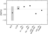 |
Fig. 5. Comparison of yields from CC SNe and SNe Ia. The mean, maximum, and minimum yields are shown for the N13 and LC18 models. |
3.3.2. Delay-time distributions
Because of their different progenitor masses and evolutionary paths, each SN Ia channel has its own delay-time distribution (DTD). We used this parameter to describe the number of SN Ia events per year and per solar mass as a function of time. A DTD thus contains information about the time delay from the formation to explosion, which is associated with the evolution of the individual binary components. It also contains information about the temporal distribution that contains all plausible candidates. The DTDs of four scenarios are shown in Fig. 6 and are briefly discussed below.
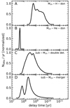 |
Fig. 6. DTDs for four different types of SN Ia as obtained from StarTrack. |
We relied on simulations from the StarTrack population synthesis code (e.g. Belczynski et al. 2008; Ruiter et al. 2009, 2014) to model the DTDs. This code evolves a simple stellar population from the zero-age main-sequence (ZAMS) over time and records the number of possible SN Ia events from various formation channels. Within our population, we find after the conversion of ∼4 × 10⁷ M⊙ of gas into stars, a fraction of ∼1% SN Ia x as opposed to 99% classical SN Ia within the Mch progenitor models, as well as ∼72% of sub-Mch occurring in double detonation (allowing for two separate evolutionary scenarios; see below) and ∼28% in double-degenerate mergers. For WD mergers, we included all binary CO WDs that merged in a Hubble time, but we excluded those with a mass of the primary WDs below 0.9 M⊙. The systems with lower-mass primaries are thought to merge without causing a supernova explosion (however, see Pakmor et al. 2021).
For the single-degenerate scenario with H-rich donors (Fig. 6, panel A), the donor star is typically in the Hertzsprung gap or is a red giant star. The evolutionary timescale of the donor is most important in setting the lower limit for the DTD. The ZAMS masses for these progenitors are typically rather low, ∼1.7 − 2.6 M⊙. This sets the timescale for the corresponding DTD because systems that have higher donor masses in our model would drop out of this progenitor channel and evolve into something else, with the shortest delay-time occurring after ∼400 Myr. In our binary population synthesis models, this only occurs in a rather narrow region of the MWD–M⊙ parameter space, although we allowed for steady H-burning. It is therefore rather difficult to build up toward the Chandrasekhar-mass limit for a large number of accreting WDs (Ruiter et al. 2009).
The He-rich donor systems involving Mch mass WD exploders (Fig. 6, panel B) have short delay-times and arise from H-stripped He-burning stars that are relatively massive (∼4−6 M⊙) on the ZAMS. They form SN Ia progenitors rather quickly after star formation (see Kromer et al. 2015, for details concerning the binary evolution calculations and delay times). In general, these systems are currently a favoured scenario for explaining SN Iax events (Jha 2017).
The evolution of the binary systems leading to sub-Mch double-detonation events (Fig. 6, panel C) differs from that of CO WD binaries that lead to violent mergers. In the former, two common-envelope events occur frequently (note the steeper power-law distribution; Ruiter et al. 2011), and the final mass-transfer RLOF phase is dynamically stable. For these systems, which are assumed to undergo a double-detonation SN Ia, donors are either He-rich WDs (either He or hybrid He-CO WDs), or H-stripped He-burning stars with masses < 1 M⊙. The binaries with WD donors typically have rather low ZAMS masses for the secondary star (≲2 M⊙), and so the progenitor configuration is not realised until > 500 Myr after star formation, leading to the second peak seen in panel C. The first peak is attributed to double detonations occurring in binaries with the He-burning stars, which generally derive from more massive progenitors in terms of the secondary star. The amount of He-rich material that is allowed to accumulate on the surface of the CO white dwarf before the He-shell detonation is dependent on the white dwarf mass, but is usually on the order of a few hundredths of a solar mass. Details are described in Ruiter et al. (2014; model P-MDS). The timescale associated with stable mass transfer is miniscule compared to the evolutionary timescale of the binary. When RLOF starts, the explosion will occur within ≲10 Myr.
Violent mergers of two CO WDs (Fig. 6, panel D) have a DTD that roughly follows a power law ∝t−1, which is to be expected because the main physical mechanism leading to decreasing orbital size in double WD mergers is set by emission of gravitational waves (see Ruiter et al. 2009, for details). A merging white dwarf system is assumed to produce a SN Ia if (i) both white dwarfs are of C-O type and (ii) at least one of the white dwarfs is above some mass threshold, in this case, 0.9 M⊙, because lower masses will not produce enough 56Ni to produce an explosion whose light curve reflects that of a typical SN Ia, including sub-luminous 91bg-like SN Ia (Ruiter et al. 2013; Shen et al. 2018; Pakmor et al. 2022, see Figs. 4, 5 and 14, respectively). The criteria that determine stability of mass transfer, that is, whether a white dwarf pair will merge or undergo stable mass transfer, when one of the white dwarfs fills its Roche lobe are defined by the properties of the individual binary. We refer to Belczynski et al. (2008). On average, we find that most mergers undergo only one common-envelope event, each of which drastically decreases the orbital separation by up to ∼2 orders of magnitude. However, one particular formation scenario of double WD mergers leads to mergers occurring 100 million years or less after star formation. These are the so-called ultra-prompt mergers (Ruiter et al. 2013). In these mergers, the same star loses its envelope twice: once while it is a regular giant-like star, and later when it is a He giant-like star. These merger progenitors, with their unique evolutionary channel, do not follow the canonical power-law distribution.
3.4. Model-data comparison
The comparison of the resulting GCE curves to the observed data was carried out as follows. We employed the goodness-of-fit statistics using the quadratic distance of each observation to the curve, weighted by the combined uncertainties in [Mn/Fe] and metallicity. The fitting algorithm is based on the emcee ensemble sampler (Foreman-Mackey et al. 2013), a Markov chain Monte Carlo (MCMC) framework that allowed us to explore the entire input parameter space using the so-called walkers. The main input parameter was Ni, the total number of SN events in channel i per solar mass formed. We applied a wide flat prior for each log Ni between 3.0 and 7.0 and allowed each of the channels to vary freely. To ensure that the chemical evolution model was physically realistic, we furthermore required that it reached solar metallicity around the birth time of the Sun, which effectively limited the total number of SNe of all channels combined and ensured a present-day [Fe/H] in agreement with expectations within the solar neighbourhood. We furthermore applied an additional prior, which ensured that the present-day SN Ia-rate was consistent with observations, such that the rate was within 0.4 × 10⁻² ± 0.2 × 10⁻² yr−1 (e.g. Prantzos et al. 2011). Initially, the walkers were evenly distributed within the bounds set by their prior to ensure that no bias was introduced by pre-selection. The sampling was then executed for 10 000 burn-in iterations, followed by 40 000 regular iterations from which the final chains were constructed. We included a pool of in total 700 walkers, meaning that the GCE model was evaluated 7 000 000 times during burn-in and 28 000 000 times during sampling. We ensured that the chosen number of walkers, as well as burn-in and sampling iterations, had no significant influence on the results because we obtained identical results for significantly longer chains.
In the context of this work, it is sufficient to estimate the ratio of all sub-Mch type explosions to the Mch models because the actual contribution of each type of progenitor is not known. Moreover, there is evidence that binary evolution population synthesis studies of the rates of SNe Ia characteristically under-predict the SN Ia rate, in particular when compared against extra-galactic rates of SN Ia (Ruiter et al. 2011, Fig. 1). We therefore refrained from restricting ourselves to the binary population synthesis model rate output alone. We furthermore reduced the dimensionality of the parameter space by only fitting the Mch-H-donor and sub-Mch double-detonation events, as well as sub-Mch mergers to the data, whereas the Mch-He donor systems were modelled by requiring the inter-channel ratios obtained at the end of the StarTrack simulations4. We recall that our methodological approach assumes that the four specific formation channels used for our binary population synthesis model (and the associated DTDs) correspond to specific nucleosynthetic yields obtained for a set of four explosion models, as discussed in Sect. 3.3. The explosion models used were chosen to feasibly match a scenario that can be naturally obtained from binary evolution. We acknowledge that other plausible SN Ia formation scenarios and DTDs might also contribute, but for this study, we only paired a set of four models (explosion model and binary evolution model) that we considered to be well matched.
The likelihood of the GCE model track [Ni/Fe] against [Fe/H]) was only evaluated in the metallicity range [Fe/H] ≳ −2.0 dex. Stars with metallicites lower than the limit have a negligible constraining power for all considered SN Ia channels (see the next section for a detailed analysis). We furthermore binned the stars in metallicity. The uncertainties in each bin were calculated from the individual abundance errors and the standard deviation.
4. Results
4.1. Galactic chemical evolution tracks
The predictions of OMEGA+ for a range of different SN Ia channel weights are presented in Fig. 7. Here we show the models calculated with CC SNe yields from the set LC18 (Limongi & Chieffi 2018), but we note that the behaviour of the distributions is very similar in the N13 set. In each panel, log Ni is varied from 3.0 to 6.0 (while the other channels are kept fixed), and the fraction relative to the total number of SNe is shown as colour.
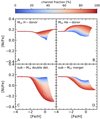 |
Fig. 7. Effects of different numbers of SN Ia on the synthetic abundance curves of [Ni/Fe]. In each panel, log Ni is varied from 3.0 to 6.0 for the respective channel, while the contributions from the remaining three channels are kept fixed. |
The main common attribute independent of the weight of each SN Ia channel is that there is no contribution at very low metallicities below ∼ − 2, which simply reflects the time delay imposed by their DTDs. However, each of the four SN Ia channels clearly has a unique signature in the [Ni/Fe] ratios. The classical Mch channel (panel A) sets in rather late, at [Fe/H] ∼ −1 dex, in the metallicity range corresponding to the transition between the thick- and thin-disc stars (e.g. Feltzing et al. 2003; Ruchti et al. 2011; Bensby et al. 2014; Bergemann et al. 2014). Decreasing the fraction of such events causes a stronger (more negative) slope towards solar [Ni/Fe] because the production of Fe is increased compared to Ni. The second Mch channel (panel B), representing Mch-He-donor type SN Ia (SN Iax), sets in very early (mainly −3 ≲ [Fe/H] ≲ −0.5). Even though the Mch-He-donor type explosions produce a high [Ni/Fe] ratio, the absolute yield is too low to influence the Galactic trend significantly enough compared to the other SN Ia channels. The strongest effect is seen for the double-detonation sub-Mch channel (panel C). Owing to their more extended DTDs, they contribute earlier, which is reflected in the lower-metallicity departure from the CC plateau. With increasing double-detonation sub-Mch fraction, the ratio of [Ni/Fe] at a given metallicity decreases. The same trend is seen for the sub-Mch merger scenario (panel D). Similar to SNe Iax, WD mergers contribute at lower metallicity, −2 ≲ [Fe/H] ≲ −0.5, where they act to decrease the Ni/Fe ratio. Hence, the contribution from WD mergers is especially interesting for the study of very low-metallicity stars.
4.2. Supernova Ia fractions
Following the procedure outlined in Sect. 3.4, we determined the sub-Mch SN Ia fractions from the posterior probability distribution constructed by fitting the observed [Ni/Fe] trend against [Fe/H] with a series of GCE models. In the procedure, we accounted for the individual abundance uncertainties of stars in the sample.
The best-fit GCE models are compared with observations in Fig. 8. In addition to our own data, we here also include the average trends based on the LTE [Ni/Fe] values from the GALAH survey5 (Buder et al. 2021) in order to aid the statistics at low metallicity. Clearly, assuming LTE or NLTE has a strong influence on the best-fit models and consequently on the resulting sub-Mch SN Ia fractions. In LTE (Fig. 8, left panel), the observations can only be described by the GCE model calculated using the core-collapse yields from Nomoto et al. (2013). This GCE model predicts a systematically decreasing [Ni/Fe] ratio with decreasing metallicity, which is qualitatively consistent with the LTE data. However, the models produce less [Ni/Fe] compared to what we see in the data at [Fe/H] ≲ −0.5. In order to reach solar [Ni/Fe] ratios, a significant contribution from classical Mch SN Ia is required, and as a result, the maximum fraction of sub-Mch SN Ia (relative to the total number of SN Ia) does not exceed ∼21 ± 3%. This is consistent with previous studies, in which the LTE abundances of Ni were used to interpret the enrichment due to different SN Ia channels, specifically in Kobayashi et al. (2020).
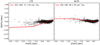 |
Fig. 8. Observed distributions of [Ni/Fe] in LTE and NLTE against [Fe/H] compared to the best-fit GCE models. The solid grey lines correspond to mean GALAH abundances. See text. |
Interestingly, the NLTE abundance ratios of [Ni/Fe] over the [Fe/H] (Fig. 8, right panel) range investigated in this work can only be explained by the GCE models that are based on the core-collapse models from Limongi & Chieffi (2018). The slightly elevated [Ni/Fe] fraction in the low-metallicity regime, as well as the mildly decreasing [Ni/Fe] trend around [Fe/H] ∼ −1, agree excellently with the NLTE abundance measurements. As emphasised in Sects. 3.3.1 and 3.4, the slight over-production of Ni (compared to Fe) at low-[Fe/H] can be balanced by sub-solar Ni/Fe fractions in sub-Mch SN Ia channels. Consequently, a very substantial fraction, 80 ± 3%, of sub-Mch SN Ia is needed to account for the NLTE [Ni/Fe] distribution. We note that the flatness of [Ni/Fe] with metallicity has been firmly established in other observational studies of the Galactic disc (Nissen & Schuster 1997; Chen et al. 2000; Adibekyan et al. 2012; Bensby et al. 2014; Hawkins et al. 2016; Jönsson et al. 2020). These studies report a tight zero-slope [Ni/Fe] trend in the disc, with a dispersion of ≲0.1 dex that is fully consistent with our present findings based on the Gaia-ESO UVES spectra. However, as we show in this work, the NLTE corrections to Ni, although not large, are strictly positive at all metallicities. Hence, taking the NLTE effects into account would also lead to mildly super-solar [Ni/Fe] ratios in other observational datasets, as we show here using the data from Bensby et al. (2014), as well as our own LTE and NLTE analysis of [Ni/Fe] abundance ratios in stellar populations of the Milky Way.
5. Discussion
Our analysis of the chemical enrichment of the Galaxy suggests that a significant fraction of sub-Mch SN Ia, ∼80%, is needed to explain the evolution of [Ni/Fe] abundance ratios in the Milky Way. This fraction is fully consistent with our earlier results (Eitner et al. 2020, 75%), although the Galactic chemical evolution model is different and we used a more comprehensive set of yields and delay-time distributions in this work.
Our findings agree with the results from Palla (2021), who reported that a dominant contribution (≳50%) from sub-Mch SN Ia describes the Galactic [Ni/Fe] evolution best. They furthermore pointed out that such a large fraction is consistent with [Mn/Fe] abundances when corrected for NLTE. We also confirm the findings by Kobayashi et al. (2020): Using the massive star yields from Nomoto et al. (2013), which are very similar to those of Kobayashi et al. (2011), and LTE abundances of Fe-group elements, there is little need for sub-Mch SN Ia because very low CC yields and classical H-donor SN Ia would be capable of explaining the Galactic evolution of [Mn/Fe] with metallicity.
Evidence for an important role of sub-Mch SN Ia in the chemical enrichment of galaxies was also reported based on studies of extragalactic stellar populations. de los Reyes et al. (2020) found that the abundances in the Sculptor dwarf galaxy are best described by a chemical evolution model based on ∼80% sub-Mch SN Ia. However, they also remarked on the role of the environment, noting that dSphs with extended SFHs tend to show higher [Mn/Fe] abundances at a similar metallicity. This conclusion qualitatively agrees with Childress et al. (2014), who reported a strong SN Ia-age dependence on the host-galaxy mass. Sanders et al. (2021), who analysed systems with a varying metallicity distribution and star formation history such as the MW Bulge or the Magellanic Clouds, also came to the conclusion that metallicity-dependent SN Ia yields are necessary to explain [Mn/Fe] abundances. They furthermore noted that only a large contribution from sub-Mch SNe is able to achieve this metallicity dependence because the [Mn/Fe] production from incomplete Si-burning is more sensitive to metallicity than the synthesis in Mch models through normal freez-out from NSE (Sanders et al. 2021; Gronow et al. 2021). Recent studies of metal-poor extragalactic globular clusters by Larsen et al. (2022) placed further emphasis on the need for sub-Mch SN Ia. They probed the [Fe/H]-regime between −1 and −3 dex through globular clusters in the Local Group and found the [Mn/Fe] ratios to be high (∼ − 0.2 dex) and approximately constant with metallicity.
Direct studies of SN light curves and spectra also provide independent information about SNe Ia progenitors. Goldstein & Kasen (2018) used time-dependent radiation transport simulations to show that the diversity of observed width-luminosity (WL) relations of SNe Ia can only be explained using sub-Mch models, whereas the classical Mch explosion can only account for bright events. Recently, Shen et al. (2021) also derived light curves and spectra of double-detonating WDs using multidimensional radiative transfer computations and found evidence that the majority of observed SNe Ia occur below Mch. Cikota et al. (2019) analysed the polarisation and line velocities of the Si II 6355 Å line using multi-epoch spectra and found a dichotomy in the polarisation properties of sub-Mch and Mch SNe, indicating that there is a significant number of observed supernovae that show clear signatures of sub-Mch. They additionally found that their observations of the peak polarisation are consistent with the Mch model from Seitenzahl et al. (2013a) as well as the sub-Mch double-det. model from Fink et al. (2010). Seitenzahl et al. (2019) studied the spatially resolved Fe XIV 5303 Å emission from three young type Ia SNe and were able to identify one of the events as an Mch and a second event as an energetic sub-Mch explosion. Support for sub-Mch explosions also stems from studies of late-type SNe spectra. Among recent studies, Flörs et al. (2020) carried out optical and near-IR spectroscopy of large samples of SN Ia systems, showing that the observed [Ni/Fe] ratios are consistent with 85% sub-Mch explosions, and only ∼11% of objects can be explained by Mch models.
6. Conclusions
We aimed to constrain the relevance of different Mch and sub-Mch SN Ia channels by comparing the predictions of Galactic chemical evolution models with new NLTE [Ni/Fe] abundance ratios in Galactic stars. The atomic model of Ni based on quantum-mechanical Ni+H collisional data from Voronov et al. (2022) was used to compute the NLTE abundances of Ni for 264 stars with high-resolution (R = 47 000) optical spectra taken within the Gaia-ESO survey. The GCE models rely on current yields from AGB stars, core-collapse SNe, SN Ia, and delay-time distributions from recent sources. Specifically, we considered a total of four Mch and sub-Mch SN Ia scenarios, including the classical single-degenerate SN Ia, SN Iax-likes, classical double detonations, and double-degenerate violent mergers of CO WDs, respectively.
First, we find that the [Ni/Fe] abundance ratios in our stellar sample show a very tight dispersion, both in LTE and in NLTE. In LTE, the trend of [Ni/Fe] is very close to solar at all metallicities probed by this work (−2.5 ≳ [Fe/H] ≳ 0.5). In NLTE, the [Ni/Fe] ratios are mildly super-solar at low metallicity, but the trends flattens to zero at [Fe/H] ≈ −1. Our LTE results are fully consistent with the Galactic [Ni/Fe] measurements in earlier studies (e.g. Nissen & Schuster 1997; Chen et al. 2000; Adibekyan et al. 2012; Bensby et al. 2014; Hawkins et al. 2016; Jönsson et al. 2020). Our work, however, is the first attempt to explore the effects of NLTE on the [Ni/Fe] over the entire metallicity range probed by the disc.
Comparing the predictions of GCE models with our LTE and NLTE data, we find that the GCE models based on the massive star yields from Limongi & Chieffi (2018) agree well with the NLTE [Ni/Fe] pattern. These models predict slightly super-solar [Ni/Fe] at low [Fe/H] and a mild decline toward the solar metallicity, as observed in the NLTE abundance ratios. The corresponding sub-Mch SN Ia fraction is 75%, which is consistent with our earlier constraints (Eitner et al. 2020). The GCE models based on the massive stars yields from Nomoto et al. (2013) do not yield a fully satisfactory agreement with Ni abundance patterns. Their [Ni/Fe] ratios are significantly lower than in LTE and NLTE data.
We emphasise that there are other SN Ia models in the literature that are not included in this study. Perets et al. (2019) presented a hybrid-disruption model for sub-Mch SN Ia that is capable of producing explosions at very low WD masses. The exploration of the other scenarios would be interesting and would merit a detailed investigation in future work.
Pairs of white dwarf binaries that are not exchanging matter can be difficult to detect in the electromagnetic spectrum, and furthermore, deriving their physical properties remains challenging. The future space-based gravitational wave observatory Laser Interferometer Space Antenna (LISA) will be able to resolve a large number of detached white dwarf binaries in our Galaxy (Nelemans et al. 2001; Ruiter et al. 2010), some of which would be likely SN Ia progenitors through the double WD merger channel discussed here. Although catching the onset of a nearby double WD merging event would be spectacular, we would have to be lucky. Nonetheless, future synergies involving LISA and current and existing surveys such as Gaia and the LSST will enable us to gain an unprecedented understanding about the properties of white dwarf binary systems well before they merge (Korol et al. 2017). This will be an important future step toward constraining the nature of SN Ia progenitor models.
Publicly available at https://github.com/becot85/JINAPyCEE
During the fitting process, we hence assumed that log NHe − don = log NH − don − 2.053.
This survey did not provide NLTE abundances of Ni.
Acknowledgments
We acknowledge the anonymous referees for the insightful report and many useful suggestions that have helped to improve the work. This work made use of the Heidelberg Supernova Model Archive (HESMA), https://hesma.h-its.org. M.B. is supported through the Lise Meitner grant from the Max Planck Society. We acknowledge support by the Collaborative Research centre SFB 881 (projects A5, A10), Heidelberg University, of the Deutsche Forschungsgemeinschaft (DFG, German Research Foundation). This project has received funding from the European Research Council (ERC) under the European Union’s Horizon 2020 research and innovation programme (Grant agreement No. 949173). This research made use of Astropy (http://www.astropy.org), a community-developed core Python package for Astronomy (Astropy Collaboration 2013, 2018). I.R.S. and A.J.R. were supported by the Australian Research Council through grant numbers FT160100028 and FT170100243, respectively. B.C. acknowledges support from the NSF grant PHY-1430152 (JINA Center for the Evolution of the Elements). This research was undertaken with the assistance of resources and services from the National Computational Infrastructure (NCI), which is supported by the Australian Government, through the National Computational Merit Allocation Scheme and the UNSW HPC Resource Allocation Scheme.
References
- Adibekyan, V. Z., Sousa, S. G., Santos, N. C., et al. 2012, A&A, 545, A32 [NASA ADS] [CrossRef] [EDP Sciences] [Google Scholar]
- Antognini, J. M. O., & Thompson, T. A. 2016, MNRAS, 456, 4219 [NASA ADS] [CrossRef] [Google Scholar]
- Astropy Collaboration (Robitaille, T. P., et al.) 2013, A&A, 558, A33 [NASA ADS] [CrossRef] [EDP Sciences] [Google Scholar]
- Astropy Collaboration (Price-Whelan, A. M., et al.) 2018, AJ, 156, 123 [Google Scholar]
- Bailer-Jones, C. A. L., Rybizki, J., Fouesneau, M., Demleitner, M., & Andrae, R. 2021, AJ, 161, 147 [Google Scholar]
- Belczynski, K., Kalogera, V., Rasio, F. A., et al. 2008, ApJS, 174, 223 [Google Scholar]
- Bensby, T., Feltzing, S., & Oey, M. S. 2014, A&A, 562, A71 [NASA ADS] [CrossRef] [EDP Sciences] [Google Scholar]
- Bergemann, M., Lind, K., Collet, R., Magic, Z., & Asplund, M. 2012, MNRAS, 427, 27 [Google Scholar]
- Bergemann, M., Ruchti, G. R., Serenelli, A., et al. 2014, A&A, 565, A89 [NASA ADS] [CrossRef] [EDP Sciences] [Google Scholar]
- Bergemann, M., Hoppe, R., Semenova, E., et al. 2021, MNRAS, 508, 2236 [NASA ADS] [CrossRef] [Google Scholar]
- Blondin, S., Bravo, E., Timmes, F. X., Dessart, L., & Hillier, D. J. 2022, A&A, 660, A96 [NASA ADS] [CrossRef] [EDP Sciences] [Google Scholar]
- Boos, S. J., Townsley, D. M., Shen, K. J., Caldwell, S., & Miles, B. J. 2021, ApJ, 919, 126 [NASA ADS] [CrossRef] [Google Scholar]
- Branch, D. 1998, ARA&A, 36, 17 [NASA ADS] [CrossRef] [Google Scholar]
- Bravo, E., & Martínez-Pinedo, G. 2012, Phys. Rev. C, 85, 055805 [NASA ADS] [CrossRef] [Google Scholar]
- Buder, S., Sharma, S., Kos, J., et al. 2021, MNRAS, 506, 150 [NASA ADS] [CrossRef] [Google Scholar]
- Carlsson, M. 1992, ASP Conf. Ser., 26, 499 [Google Scholar]
- Chen, Y. Q., Nissen, P. E., Zhao, G., Zhang, H. W., & Benoni, T. 2000, A&AS, 141, 491 [NASA ADS] [CrossRef] [EDP Sciences] [Google Scholar]
- Chiappini, C., Matteucci, F., & Gratton, R. 1997, ApJ, 477, 765 [Google Scholar]
- Childress, M. J., Wolf, C., & Zahid, H. J. 2014, MNRAS, 445, 1898 [Google Scholar]
- Cikota, A., Patat, F., Wang, L., et al. 2019, MNRAS, 490, 578 [NASA ADS] [CrossRef] [Google Scholar]
- Côté, B., & Ritter, C. 2018, Astrophysics Source Code Library [record ascl:1806.018] [Google Scholar]
- Côté, B., O’Shea, B. W., Ritter, C., Herwig, F., & Venn, K. A. 2017, ApJ, 835, 128 [Google Scholar]
- Côté, B., Silvia, D. W., O’Shea, B. W., Smith, B., & Wise, J. H. 2018, ApJ, 859, 67 [CrossRef] [Google Scholar]
- Côté, B., Lugaro, M., Reifarth, R., et al. 2019, ApJ, 878, 156 [CrossRef] [Google Scholar]
- Cristallo, S., Straniero, O., & Piersanti, L. 2015, ASP Conf. Ser., 497, 301 [NASA ADS] [Google Scholar]
- de los Reyes, M. A. C., Kirby, E. N., Seitenzahl, I. R., & Shen, K. J. 2020, ApJ, 891, 85 [NASA ADS] [CrossRef] [Google Scholar]
- Eitner, P., Bergemann, M., Hansen, C. J., et al. 2020, A&A, 635, A38 [NASA ADS] [CrossRef] [EDP Sciences] [Google Scholar]
- Feltzing, S., Bensby, T., & Lundström, I. 2003, A&A, 397, L1 [NASA ADS] [CrossRef] [EDP Sciences] [Google Scholar]
- Fink, M., Röpke, F. K., Hillebrandt, W., et al. 2010, A&A, 514, A53 [NASA ADS] [CrossRef] [EDP Sciences] [Google Scholar]
- Fink, M., Kromer, M., Seitenzahl, I. R., et al. 2014, MNRAS, 438, 1762 [NASA ADS] [CrossRef] [Google Scholar]
- Flörs, A., Spyromilio, J., Taubenberger, S., et al. 2020, MNRAS, 491, 2902 [NASA ADS] [Google Scholar]
- Foley, R. J., Challis, P. J., Chornock, R., et al. 2013, ApJ, 767, 57 [Google Scholar]
- Foreman-Mackey, D., Hogg, D. W., Lang, D., & Goodman, J. 2013, PASP, 125, 306 [Google Scholar]
- Gaia Collaboration (Brown, A. G. A., et al.) 2021, A&A, 649, A1 [NASA ADS] [CrossRef] [EDP Sciences] [Google Scholar]
- Gent, M. R., Bergemann, M., Serenelli, A., et al. 2022, A&A, 658, A147 [NASA ADS] [CrossRef] [EDP Sciences] [Google Scholar]
- Gerber, J. M., Magg, E., Plez, B., et al. 2023, A&A, 669, A43 [NASA ADS] [CrossRef] [EDP Sciences] [Google Scholar]
- Gibson, B. K., Fenner, Y., Renda, A., Kawata, D., & Lee, H.-C. 2003, PASA, 20, 401 [NASA ADS] [CrossRef] [Google Scholar]
- Gilmore, G., Randich, S., Worley, C. C., et al. 2022, A&A, 666, A120 [NASA ADS] [CrossRef] [EDP Sciences] [Google Scholar]
- Goldstein, D. A., & Kasen, D. 2018, ApJ, 852, L33 [NASA ADS] [CrossRef] [Google Scholar]
- Gronow, S., Collins, C., Ohlmann, S. T., et al. 2020, A&A, 635, A169 [NASA ADS] [CrossRef] [EDP Sciences] [Google Scholar]
- Gronow, S., Côté, B., Lach, F., et al. 2021, A&A, 656, A94 [NASA ADS] [CrossRef] [EDP Sciences] [Google Scholar]
- Hawkins, K., Masseron, T., Jofré, P., et al. 2016, A&A, 594, A43 [NASA ADS] [CrossRef] [EDP Sciences] [Google Scholar]
- Heger, A., & Woosley, S. E. 2010, ApJ, 724, 341 [Google Scholar]
- Hillebrandt, W., Kromer, M., Röpke, F. K., & Ruiter, A. J. 2013, Front. Phys., 8, 116 [Google Scholar]
- Iben, I., Jr., Nomoto, K., Tornambe, A., & Tutukov, A. V. 1987, ApJ, 317, 717 [NASA ADS] [CrossRef] [Google Scholar]
- Jha, S. W. 2017, in Handbook of Supernovae, eds. A. W. Alsabti, & P. Murdin, 375 [CrossRef] [Google Scholar]
- Jiang, J.-A., Doi, M., Maeda, K., et al. 2017, Nature, 550, 80 [CrossRef] [Google Scholar]
- Jönsson, H., Holtzman, J. A., Allende Prieto, C., et al. 2020, AJ, 160, 120 [Google Scholar]
- Jordan, G. C., IV, Perets, H. B., Fisher, R. T., & van Rossum, D. R. 2012, ApJ, 761, L23 [NASA ADS] [CrossRef] [Google Scholar]
- Karakas, A. I. 2010, MNRAS, 403, 1413 [NASA ADS] [CrossRef] [Google Scholar]
- Kennicutt, R. C., Jr. 1998, ApJ, 498, 541 [Google Scholar]
- Khokhlov, A. M. 1991, A&A, 245, 114 [NASA ADS] [Google Scholar]
- Kirby, E. N., Xie, J. L., Guo, R., et al. 2019, ApJ, 881, 45 [NASA ADS] [CrossRef] [Google Scholar]
- Kobayashi, C., Tsujimoto, T., & Nomoto, K. 2000, ApJ, 539, 26 [NASA ADS] [CrossRef] [Google Scholar]
- Kobayashi, C., Umeda, H., Nomoto, K., Tominaga, N., & Ohkubo, T. 2006, ApJ, 653, 1145 [NASA ADS] [CrossRef] [Google Scholar]
- Kobayashi, C., Karakas, A. I., & Umeda, H. 2011, MNRAS, 414, 3231 [Google Scholar]
- Kobayashi, C., Leung, S.-C., & Nomoto, K. 2020, ApJ, 895, 138 [CrossRef] [Google Scholar]
- Korol, V., Rossi, E. M., Groot, P. J., et al. 2017, MNRAS, 470, 1894 [NASA ADS] [CrossRef] [Google Scholar]
- Kromer, M., Fink, M., Stanishev, V., et al. 2013a, MNRAS, 429, 2287 [NASA ADS] [CrossRef] [Google Scholar]
- Kromer, M., Pakmor, R., Taubenberger, S., et al. 2013b, ApJ, 778, L18 [NASA ADS] [CrossRef] [Google Scholar]
- Kromer, M., Ohlmann, S. T., Pakmor, R., et al. 2015, MNRAS, 450, 3045 [NASA ADS] [CrossRef] [Google Scholar]
- Kromer, M., Ohlmann, S., & Röpke, F. K. 2017, Mem. Soc. Astron. It., 88, 312 [NASA ADS] [Google Scholar]
- Kroupa, P. 2001, MNRAS, 322, 231 [NASA ADS] [CrossRef] [Google Scholar]
- Lach, F., Röpke, F. K., Seitenzahl, I. R., et al. 2020, A&A, 644, A118 [NASA ADS] [CrossRef] [EDP Sciences] [Google Scholar]
- Larsen, S. S., Eitner, P., Magg, E., et al. 2022, A&A, 660, A88 [NASA ADS] [CrossRef] [EDP Sciences] [Google Scholar]
- Limongi, M., & Chieffi, A. 2018, ApJS, 237, 13 [NASA ADS] [CrossRef] [Google Scholar]
- Lind, K., Bergemann, M., & Asplund, M. 2012, MNRAS, 427, 50 [Google Scholar]
- Livne, E. 1990, ApJ, 354, L53 [Google Scholar]
- Magg, E., Bergemann, M., Serenelli, A., et al. 2022, A&A, 661, A140 [NASA ADS] [CrossRef] [EDP Sciences] [Google Scholar]
- Matteucci, F. 2004, in Origin and Evolution of the Elements, eds. A. McWilliam, & M. Rauch, 85 [Google Scholar]
- Matteucci, F., & Greggio, L. 1986, A&A, 154, 279 [NASA ADS] [Google Scholar]
- McWilliam, A., Piro, A. L., Badenes, C., & Bravo, E. 2018, ApJ, 857, 97 [NASA ADS] [CrossRef] [Google Scholar]
- Nelemans, G., Yungelson, L. R., & Portegies Zwart, S. F. 2001, A&A, 375, 890 [NASA ADS] [CrossRef] [EDP Sciences] [Google Scholar]
- Nissen, P. E., & Schuster, W. J. 1997, A&A, 326, 751 [NASA ADS] [Google Scholar]
- Nomoto, K., Tominaga, N., Umeda, H., Kobayashi, C., & Maeda, K. 2006, Nucl. Phys. A, 777, 424 [CrossRef] [Google Scholar]
- Nomoto, K., Kobayashi, C., & Tominaga, N. 2013, ARA&A, 51, 457 [CrossRef] [Google Scholar]
- Pakmor, R., Kromer, M., Taubenberger, S., et al. 2012, ApJ, 747, L10 [NASA ADS] [CrossRef] [Google Scholar]
- Pakmor, R., Zenati, Y., Perets, H. B., & Toonen, S. 2021, MNRAS, 503, 4734 [Google Scholar]
- Pakmor, R., Callan, F. P., Collins, C. E., et al. 2022, MNRAS, 517, 5260 [NASA ADS] [CrossRef] [Google Scholar]
- Palla, M. 2021, MNRAS, 503, 3216 [Google Scholar]
- Perets, H. B., Zenati, Y., Toonen, S., & Bobrick, A. 2019, ArXiv e-prints [arXiv:1910.07532] [Google Scholar]
- Phillips, M. M. 1993, ApJ, 413, L105 [Google Scholar]
- Prantzos, N. 2008, in EAS Pub. Ser., 32, 311 [NASA ADS] [CrossRef] [EDP Sciences] [Google Scholar]
- Prantzos, N., Boehm, C., Bykov, A. M., et al. 2011, Rev. Mod. Phys., 83, 1001 [NASA ADS] [CrossRef] [Google Scholar]
- Prantzos, N., Abia, C., Limongi, M., Chieffi, A., & Cristallo, S. 2018, MNRAS, 476, 3432 [Google Scholar]
- Randich, S., Gilmore, G., Magrini, L., et al. 2022, A&A, 666, A121 [NASA ADS] [CrossRef] [EDP Sciences] [Google Scholar]
- Riess, A. G., Filippenko, A. V., Challis, P., et al. 1998, AJ, 116, 1009 [Google Scholar]
- Riess, A. G., Yuan, W., Macri, L. M., et al. 2022, ApJ, 934, L7 [NASA ADS] [CrossRef] [Google Scholar]
- Röpke, F. K., Kromer, M., Seitenzahl, I. R., et al. 2012, ApJ, 750, L19 [CrossRef] [Google Scholar]
- Ruchti, G. R., Fulbright, J. P., Wyse, R. F. G., et al. 2011, ApJ, 737, 9 [NASA ADS] [CrossRef] [Google Scholar]
- Ruiter, A. J. 2019, Proc. IAU Symp., 15, 1 [CrossRef] [Google Scholar]
- Ruiter, A. J., Belczynski, K., & Fryer, C. 2009, ApJ, 699, 2026 [Google Scholar]
- Ruiter, A. J., Belczynski, K., Benacquista, M., Larson, S. L., & Williams, G. 2010, ApJ, 717, 1006 [NASA ADS] [CrossRef] [Google Scholar]
- Ruiter, A. J., Belczynski, K., Sim, S. A., et al. 2011, MNRAS, 417, 408 [CrossRef] [Google Scholar]
- Ruiter, A. J., Sim, S. A., Pakmor, R., et al. 2013, MNRAS, 429, 1425 [NASA ADS] [CrossRef] [Google Scholar]
- Ruiter, A. J., Belczynski, K., Sim, S. A., Seitenzahl, I. R., & Kwiatkowski, D. 2014, MNRAS, 440, L101 [NASA ADS] [CrossRef] [Google Scholar]
- Rybizki, J., Just, A., & Rix, H.-W. 2017, A&A, 605, A59 [NASA ADS] [CrossRef] [EDP Sciences] [Google Scholar]
- Sanders, J. L., Belokurov, V., & Man, K. T. F. 2021, MNRAS, 506, 4321 [NASA ADS] [CrossRef] [Google Scholar]
- Seitenzahl, I. R., Cescutti, G., Röpke, F. K., Ruiter, A. J., & Pakmor, R. 2013a, A&A, 559, L5 [NASA ADS] [CrossRef] [EDP Sciences] [Google Scholar]
- Seitenzahl, I. R., Ciaraldi-Schoolmann, F., Röpke, F. K., et al. 2013b, MNRAS, 429, 1156 [NASA ADS] [CrossRef] [Google Scholar]
- Seitenzahl, I. R., Ghavamian, P., Laming, J. M., & Vogt, F. P. A. 2019, Phys. Rev. Lett., 123, 041101 [CrossRef] [Google Scholar]
- Semenova, E., Bergemann, M., Deal, M., et al. 2020, A&A, 643, A164 [NASA ADS] [CrossRef] [EDP Sciences] [Google Scholar]
- Shen, K. J., Kasen, D., Miles, B. J., & Townsley, D. M. 2018, ApJ, 854, 52 [Google Scholar]
- Shen, K. J., Boos, S. J., Townsley, D. M., & Kasen, D. 2021, ApJ, 922, 68 [NASA ADS] [CrossRef] [Google Scholar]
- Sim, S. A., Röpke, F. K., Hillebrandt, W., et al. 2010, ApJ, 714, L52 [Google Scholar]
- Taubenberger, S. 2017, in The Extremes of Thermonuclear Supernovae, eds. A. W. Alsabti, & P. Murdin, 317 [Google Scholar]
- Timmes, F. X., Woosley, S. E., & Weaver, T. A. 1995, ApJS, 98, 617 [NASA ADS] [CrossRef] [Google Scholar]
- Tinsley, B. M. 1980, Fund. Cosmic Phys., 5, 287 [Google Scholar]
- Tominaga, N., Umeda, H., & Nomoto, K. 2007, ApJ, 660, 516 [NASA ADS] [CrossRef] [Google Scholar]
- Toonen, S., Perets, H. B., & Hamers, A. S. 2018, A&A, 610, A22 [NASA ADS] [CrossRef] [EDP Sciences] [Google Scholar]
- Umeda, H., & Nomoto, K. 2002, ApJ, 565, 385 [Google Scholar]
- Voronov, Y. V., Yakovleva, S. A., & Belyaev, A. K. 2022, ApJ, 926, 173 [NASA ADS] [CrossRef] [Google Scholar]
- Weinberg, D. H., Andrews, B. H., & Freudenburg, J. 2017, ApJ, 837, 183 [NASA ADS] [CrossRef] [Google Scholar]
- Yates, R. M., Henriques, B., Thomas, P. A., et al. 2013, MNRAS, 435, 3500 [CrossRef] [Google Scholar]
All Figures
|
Fig. 1. Best-fit line profiles for two diagnostic lines of Ni for three representative stars at metallicities [Fe/H] = −0.34, −0.55, and −1.05. |
| In the text | |
|
Fig. 2. Ni NLTE corrections as a function of metallicity for three representative stellar model atmospheres averaged over diagnostic lines of Ni I in the optical wavelength range. |
| In the text | |
|
Fig. 3. Trends of [Ni/Fe] against metallicity [Fe/H], calculated in LTE (left) and NLTE (right). |
| In the text | |
|
Fig. 4. Comparison of the integrated yields from CC SNe from Limongi & Chieffi (2018) and Nomoto et al. (2013). Top row: yields as a function of stellar mass, averaged over metallicity. Bottom panel: mass-averaged yields as a function of metallicity. |
| In the text | |
|
Fig. 5. Comparison of yields from CC SNe and SNe Ia. The mean, maximum, and minimum yields are shown for the N13 and LC18 models. |
| In the text | |
|
Fig. 6. DTDs for four different types of SN Ia as obtained from StarTrack. |
| In the text | |
|
Fig. 7. Effects of different numbers of SN Ia on the synthetic abundance curves of [Ni/Fe]. In each panel, log Ni is varied from 3.0 to 6.0 for the respective channel, while the contributions from the remaining three channels are kept fixed. |
| In the text | |
|
Fig. 8. Observed distributions of [Ni/Fe] in LTE and NLTE against [Fe/H] compared to the best-fit GCE models. The solid grey lines correspond to mean GALAH abundances. See text. |
| In the text | |
Current usage metrics show cumulative count of Article Views (full-text article views including HTML views, PDF and ePub downloads, according to the available data) and Abstracts Views on Vision4Press platform.
Data correspond to usage on the plateform after 2015. The current usage metrics is available 48-96 hours after online publication and is updated daily on week days.
Initial download of the metrics may take a while.