| Issue |
A&A
Volume 676, August 2023
|
|
|---|---|---|
| Article Number | A134 | |
| Number of page(s) | 11 | |
| Section | Galactic structure, stellar clusters and populations | |
| DOI | https://doi.org/10.1051/0004-6361/202346474 | |
| Published online | 23 August 2023 | |
A Bayesian estimation of the Milky Way’s circular velocity curve using Gaia DR3
1
NICPB, Rävala 10, Tallinn 10143, Estonia
e-mail: This email address is being protected from spambots. You need JavaScript enabled to view it.
2
Tallinn University of Technology, Ehitajate tee 5, Tallinn 19086, Estonia
3
Tartu Observatory, University of Tartu, Observatooriumi 1, Tõravere 61602, Estonia
e-mail: This email address is being protected from spambots. You need JavaScript enabled to view it.
4
Instituto de Astrofísica de Canarias, C/Vía Láctea s/n, 38205 La Laguna, Tenerife, Spain
5
Universidad de La Laguna, Dpto. Astrofísica, Avenida Astrofísico Francisco Sánchez, 38206 La Laguna, Tenerife, Spain
Received:
21
March
2023
Accepted:
27
June
2023
Abstract
Aims. Our goal is to calculate the circular velocity curve of the Milky Way, along with corresponding uncertainties that quantify various sources of systematic uncertainty in a self-consistent manner.
Methods. The observed rotational velocities are described as circular velocities minus the asymmetric drift. The latter is described by the radial axisymmetric Jeans equation. We thus reconstruct the circular velocity curve between Galactocentric distances from 5 kpc to 14 kpc using a Bayesian inference approach. The estimated error bars quantify uncertainties in the Sun’s Galactocentric distance and the spatial-kinematic morphology of the tracer stars. As tracers, we used a sample of roughly 0.6 million stars on the red giant branch stars with six-dimensional phase-space coordinates from Gaia Data Release 3 (DR3). More than 99% of the sample is confined to a quarter of the stellar disc with mean radial, rotational, and vertical velocity dispersions of (35 ± 18) km s−1, (25 ± 13) km s−1, and (19 ± 9) km s−1, respectively.
Results. We find a circular velocity curve with a slope of 0.4 ± 0.6 km s−1 kpc−1, which is consistent with a flat curve within the uncertainties. We further estimate a circular velocity at the Sun’s position of vc(R0) = 233 ± 7 km s−1 and that a region in the Sun’s vicinity, characterised by a physical length scale of ∼1 kpc, moves with a bulk motion of VLSR = 7 ± 7 km s−1. Finally, we estimate that the dark matter (DM) mass within 14 kpc is log10 MDM(R < 14kpc)/ M⊙ =(11.2+2.0-2.3) and the local spherically averaged DM density is ρDM(RO)=(0.41+0.10-0.09) GeV cm-3 = (0.011+0.003-0.002) M⊙pc-3. In addition, the effect of biased distance estimates on our results is assessed.
Key words: Galaxy: kinematics and dynamics / Galaxy: disk / methods: statistical
© The Authors 2023
 Open Access article, published by EDP Sciences, under the terms of the Creative Commons Attribution License (https://creativecommons.org/licenses/by/4.0), which permits unrestricted use, distribution, and reproduction in any medium, provided the original work is properly cited.
This article is published in open access under the Subscribe to Open model. This email address is being protected from spambots. You need JavaScript enabled to view it. to support open access publication.
1. Introduction
The rotation of stars and gas in galactic discs has been extensively used as a kinematical tracer of matter distribution of external galaxies and our own Galaxy, the Milky Way (MW) (Kuzmin 2022). Several recent studies (Mróz et al. 2019; Eilers et al. 2019; Chrobáková et al. 2020; Ablimit et al. 2020; Khanna et al. 2023; Gaia Collaboration 2023; Wang et al. 2022; Zhou et al. 2023) have measured the stellar disc rotation in the MW using stellar data from the Gaia satellite (Gaia Collaboration 2016). These studies differ in the samples of stars used as a tracer and/or in the methodology and assumptions employed. Moreover, some of the cited studies provided rotational (azimuthal) velocities, whereas the others presented circular ones. The former are direct measurements and no underlying assumptions are made with respect to the shape or time dependence of the MW’s gravitational potential. On the other hand, circular velocities assume a stationary gravitational potential that exhibits axial symmetry. Moreover, these are the velocities that should be used to derive the total or dynamical matter distribution. The modelling assumptions can therefore bias the determination of the total and dark matter content in our Galaxy.
The amount of phase space data currently available is large, and statistics is generally not the limiting factor for studies of the dynamics of the MW stellar disc. The limiting factor is instead systematic errors, such as the Sun’s Galactocentric distance or the adoption of incorrect modelling assumptions. In this paper, we present a Bayesian inference approach to estimate the circular velocity curve of our Galaxy that allows the straightforward incorporation of systematic and statistical sources of uncertainty, which are both treated as nuisance parameters. In this way, we provide, for the first time, a circular velocity curve with errorbars that self-consistently include uncertainties in the Sun’s Galactocentric distance and in the spatial-kinematic structure of the stellar disc. Therefore, our uncertain knowledge about astrophysical parameters is propagated through Bayes’ theorem to the determination of the circular velocity curve and, subsequently, to the estimation of the dark matter density profile in our Galaxy. Taking into account the uncertainties about how dark matter is distributed in the MW is essential for interpreting the results of dark matter particle searches (see e.g. Benito et al. 2017).
The Bayesian inference approach presented here is a flexible method that models the observed rotational or azimuthal velocity at a given Galactocentric distance as the difference between the circular velocity and the asymmetric drift component. The latter velocity component is obtained from the stationary, axisymmetric radial Jeans equation under the assumption of symmetry above and below the Galactic plane. Observed and modelled azimuthal velocities are then compared by means of the Bayes theorem. The paper is divided as follows. Section 2 describes the data; Sect. 3 presents the Bayesian methodology. The results are presented in Sect. 4, and we conclude in Sect. 5.
2. Data
2.1. Red giant branch stars
We used astrometric data and radial velocities from Gaia data release 3 (DR3) for 665 660 stars in the red giant branch (RGB). These stars are old and have relatively large velocity dispersion. Thus, they are less susceptible to perturbations. They are also bright enough to have measured radial velocities out to large distances. Specifically, we used the same sample of almost six million RGB stars as in Gaia Collaboration (2023) to which we performed additional spatial and kinematic cuts.
In the following we briefly describe how the RGB sample was obtained and we refer readers to the original paper Gaia Collaboration (2023) for a thorough description. Red giants are identified as stars with effective temperatures between 3000 K and 5500 K and surface gravity satisfying the condition log g < 3. Both stellar parameters are provided as data products in Gaia DR3 (Andrae et al. 2023). Using these first selection criteria, we obtained 11 576 957 sources. We then selected RGB stars with good astrometric data as measured by the fidelity parameter fa given in Rybizki et al. (2022) and we removed stars with fa ≤ 0.5, thus remaining with 6 586 329 stars. After this, we performed a cut in height above and below the Galactic plane, |z|< 0.2 kpc (which removes ca. 4.5M stars), a cut in Galactocentric distances 5 kpc < R < 14 kpc (removing ca. 84k stars), and a cut in heliocentric velocity |v − v⊙| < 210 km s−11. The latter cut removed roughly 28k stars. The z and velocity cuts are applied to remove halo stars (Helmi et al. 2018; Thomas et al. 2019). The cut in height also avoids large density and velocity gradients in the z-coordinate, thus making the derivatives with respect to z in the Jeans equation negligible (see Eq. (3)). We note that the scale height of the thin disc is roughly 250 pc (Bland-Hawthorn & Gerhard 2016).
We used GSP-Phot distances (Andrae et al. 2023) instead of the inverse of the parallax due to noisy parallax measurements. As shown in the left panel of Fig. 1, the GSP-Phot distances are significantly underestimated at large distances from the Sun (see also Andrae et al. 2023; Fouesneau et al. 2023). This would lead to artificially lower circular velocities and thus to a steeper slope of the estimated circular velocity curve. To reduce this bias, we imposed a tight constraint on the quality of the parallax measurements, namely ϖ/σϖ > 20. This cut-off removed approximately 1.3M stars and suppressed the systematic underestimation of the distances, in fact leading to a slight overestimation. To assess the dependence of our results on inaccurate distances, we further performed the same analysis using a less stringent quality cut on parallaxes and ‘photogeo’ distances from Bailer-Jones et al. (2021; henceforth referred to as BJ21). Photogeo distances suffer from underestimation when including measurements with ϖ/σϖ ≲ 20 (see the right panel of Fig. 1). In the end, we are left with a final sample of 665 660 stars which is shown in Fig. 2.
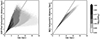 |
Fig. 1. Bias in different distance estimates. Left: GSP-Phot heliocentric distances as a function of parallax inverse. The colour bar shows the mean parallax quality inside each pixel. The quality cut used in this paper corresponds to log10(ϖ/σϖ) > 1.301. Right: same but for photogeo heliocentric distances by Bailer-Jones et al. (2021). |
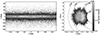 |
Fig. 2. Spatial distribution of the final red giants sample. Left: distribution in the Galactic longitude (ℓ) and latitude (b) plane. The colour bar shows the number density of stars per pixel. Each pixel has a size of 1 degree in both latitude and longitude. Right: same but projected into the Galactic plane. Each pixel has a size of 0.05 kpc and 0.06 kpc in the x and y coordinates, respectively. In this figure, the Galactic centre is located at (0, 0), the Sun is located at ( − 8.277, 0) and the rotation of the Galaxy is clockwise. We added dashed, black circles at 5 kpc, R0 = 8.277 kpc, 12 kpc and 14 kpc to ease visualisation. For the transformation to Galactocentric coordinades, we adopt R0 = 8.277 kpc, z0 = 25 pc and v⊙ = (11.1, 251.5, 8.59) km s−1. |
2.2. Galactocentric frame
2.2.1. Galactocentric transformation
We transformed RGB stars from a heliocentric to a Galactocentric reference frame. We used a right-handed Galactocentric coordinate system (x, y, z), with the Sun located at negative x, y pointing in the direction of the Galactic rotation and z towards the North Galactic Pole. In order to define this new frame and perform the transformation correctly, we assumed solar orbital parameters (R0, z0, U⊙, V⊙, W⊙) from contemporary literature. First, we treated the Galactocentric distance R0 as a nuisance parameter of the analysis in order to account for uncertainties in its determination. In particular, we used a uniform prior range R0 ∈ [7.8 − 8.5] kpc that encompasses recent estimates with their corresponding uncertainties (Do et al. 2019; GRAVITY Collaboration 2021, 2019, 2020, 2022; Abuter et al. 2018; Leung et al. 2022). Our intention was not to constrain the value of R0, but rather to show how the uncertainty in this parameter, which is encoded in the prior, propagates into the circular velocity curve. For this reason, we remained agnostic about the actual value of R0 and adopted a uniform distribution that encompasses the most recent R0 estimations within 2σ uncertainty. Second, for the height of the Sun over the Galactic plane z0, we assumed a value of 25 pc (Jurić et al. 2008)2. The transformation from spherical coordinates in ICRS to a Galactocentric Cartesian setting was done as described in Johnson & Soderblom (1987) and Hobbs et al. (2018).
Finally, the radial velocity measurements from Gaia also allow us to construct the full 3D space velocities and then transform them to a new frame by using the Sun’s Galactocentric velocity. Under the assumption that Sg A* is at rest at the Galactic centre, the y and z components of the total solar velocity vector are derived from the proper motion of Sg A*, as measured in Reid & Brunthaler (2020), in combination with the adopted value of R0. On the other hand, for the x-component of the velocity, we adopted the value from Schönrich et al. (2010). We have not corrected this value for the offset in radial velocity between the radio-to-infrared reference frames determined by the GRAVITY Collaboration (GRAVITY Collaboration 2019, 2020, 2021, 2022) as suggested in Drimmel & Poggio (2018). There are many possible sources for this systematic offset and, in any case, it is compatible with zero at the 2σ level (GRAVITY Collaboration 2022). In this way, we obtain the following vector
 (1)
(1)
where U⊙, V⊙, W⊙ correspond to the velocity components in the Galactocentric x, y, and z-directions, respectively. As U⊙ corresponds to the radial motion of the Sun towards the Galactic centre, we implicitly assumed that the LSR has no such motion.
Using Gaia measurements for right ascension, declination, and radial velocity, and the GSP-Phot distances with a quality parallax cut of ϖ/σϖ > 20, we transformed the proper motions and radial velocities first to Cartesian velocities in a similar way as was done in Johnson & Soderblom (1987) and Hobbs et al. (2018). Finally, we switched to Galactocentric cylindrical coordinates (R, ϕ, z, vR, vϕ, vz).
The left panel of Fig. 3 shows the mean observed rotational velocities in the Galactic plane. The right panel of the same figure depicts the mean axisymmetric radial and azimuthal velocity dispersions. Figure 4 shows the mean azimuthal and radial velocities. In both figures uncertainties are calculated by bootstrap resampling and are given by half the interval between the 16th and 84th percentiles of the corresponding distribution. As shown in the right panel of the last figure, the bulk motion of the stars in the radial direction exhibits an oscillatory pattern with an amplitude of roughly 5 km s−1. This was already reported in Gaia DR2 (Gaia Collaboration 2018) and might be a kinematic signature of the spiral arms or the result of interaction with a perturber. We leave for future work a careful study of the origin of this intriguing oscillation in the radial velocities.
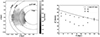 |
Fig. 3. Distribution of the mean observed rotational velocity vϕ inside x–y pixels for our final sample of RGB stars (left). The size of the bin is 150 pc in both x and y coordinates, respectively. We added dashed, black circles at 5 kpc, R0 = 8.277 kpc, 12 and 14 kpc to ease visualisation. Square root of the radial and azimuthal diagonal components of the velocity dispersion tensor in radial bins of 1 kpc (right). |
 |
Fig. 4. Mean azimuthal (left) and radial (right) velocities as a function of Galactocentric distance R. As in Fig. 3, errorbars are calculated via bootstrap (see text for details). |
2.2.2. Binning
We treated the Sun’s Galactocentric distance as a free parameter in our analysis. Varying R0 translates into a variation of the R coordinate of the RGB stars. For this reason, we distributed the RGB sample in bins defined in the adimensional coordinate x = R/R0. This mitigates the shift of the red giants’ R coordinate when varying R0. Thus, for different R0 values, a given x bin contains approximately the same stars (Benito et al. 2019). Furthermore, we note that by marginalising over the azimuthal coordinate ϕ, the rotational velocity in the Galactic disc is treated as a purely radially dependent observable.
In total, we defined eight bins from x = 5/8.277 to x = 14/8.277 with a step of Δx = 1/8.277. Observed rotational (azimuthal) velocities inside each bin approximately follow a Gaussian distribution as shown in Fig. 5. In this figure, we plot the distribution of observed velocities inside two bins: the bin where the distribution deviates most from a Gaussian and a randomly selected bin. The rotational velocity inside each bin is defined by the mean. The associated uncertainties are calculated by bootstrap resamplings and are given by half the interval between the 16th and 84th percentiles of the velocity distributions.
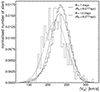 |
Fig. 5. Distribution of vϕ inside the last radial bin where the distribution of values deviates most from a Gaussian distribution (orange) and a randomly selected bin (blue). The dashed lines depict the best-fitted Gaussian of the rotational velocity inside each particular bin. |
3. Methodology
3.1. Axisymmetric kinematic model
Inside each radial bin, we modeled the mean rotational or azimuthal velocity as
 (2)
(2)
where vc is the circular velocity or the velocity of a star moving in a circular orbit and va is the asymmetric drift. The latter accounts for the diffusion of stars in phase-space as the stars orbit the Galaxy and streaming or bulk motions inside the disc. Neglecting large scale non-axisymmetric features, the asymmetric drift component can be obtained from the radial Jeans equation under the assumption that the MW is in a steady-state and has an axisymmetric gravitational potential (Binney & Tremaine 2008). If we further expect the density distribution to be symmetric with respect to the Galactic plane, the Jeans equation takes the following form
 (3)
(3)
Substituting  3 and assuming
  , we further obtain
 (4)
(4)
We have checked the latter assumption explicitly and observed that the measured values of  are at least two orders of magnitude larger than the measured
  .
.
In traditional approaches, circular velocities in radial bins are calculated by plugging numbers into Eq. (4). Circular velocity values between bins are correlated as the radial dependence of the density profile and radial velocity dispersion are described by exponential functions. In the proposed new approach, we add Eq. (2) to transform the problem into an inference procedure. In this way, we can introduce free parameters such as scale lengths of the exponential functions and/or the Sun’s Galactocentric distance R0. The fitting procedure introduces an additional correlation between the bins. Nonetheless, we found that if we fix all free parameters of the analysis (i.e. scale lengths and R0), the traditional and new approaches give the same circular velocity curve.
By expanding the difference of squares on the right hand side and introducing Eq. (2), we arrive to the following expression for the asymmetric drift
![Mathematical equation: $$ \begin{aligned} { v}_{\rm a} = \frac{\sigma _{R}^{*2}}{{ v}_{\rm c} + \overline{{ v}_\phi }}\left[\frac{\sigma _\phi ^{*2}}{\sigma _R^{*2}}-1-\frac{\partial \ln \nu }{\partial \ln R}-\frac{\partial \ln (\sigma _R^{*2})}{\partial \ln R}-\frac{R}{\sigma _R^{*2}}\frac{\partial \overline{{ v}_R{ v}_z}}{\partial z}\right]. \end{aligned} $$](/articles/aa/full_html/2023/08/aa46474-23/aa46474-23-eq11.gif) (5)
(5)
The sum  in the denominator is often approximated as ≈2vc (Binney & Tremaine 2008). Nonetheless, we leave it as it is and estimate
  as the mean rotational velocity inside each bin. In addition to this, the diagonal components of the velocity-dispersion tensor
  and
and  are also calculated directly from the data, and they correspond to the variance of the azimuthal and radial velocity in the bin respectively. For the 3rd component inside the brackets of Eq. (5), the number density distribution ν is described by an exponential profile, namely ν ∝ exp( − R/hR) with hR the disc scale radius. Notice that in the 4th component we describe
  as
as  , where hσ is the scale length of the radial velocity dispersion. Finally, after taking the derivatives with respect to lnR in (5), we are left with the following equation
![Mathematical equation: $$ \begin{aligned} { v}_{\rm a} = \frac{\sigma _R^{*2}}{{ v}_{\rm c} + \overline{{ v}_\phi }}\left[\frac{\sigma _\phi ^{*2}}{\sigma _R^{*2}}-1+R\left(\frac{1}{h_r} + \frac{2}{h_\sigma }\right)\right]. \end{aligned} $$](/articles/aa/full_html/2023/08/aa46474-23/aa46474-23-eq18.gif) (6)
(6)
We neglect the last term of (5) in our axisymmetric treatment of the rotation curve derivation as  . This is motivated because the radial and vertical motions are expected to decouple for circular orbits near the disc when the velocity ellipsoid is aligned with the Galactic plane (Bovy, in prep.). In reality, however, this is not necessarily true (e.g. some general models are provided by Tempel & Tenjes 2006; Kipper et al. 2016). In any case, our cut in z-coordinate |z|< 0.2 kpc minimises gradients in the vertical direction. Furthermore, the inclusion of this term changes the final circular velocity at the percent level, as shown in Eilers et al. (2019).
3.2. Circular velocity fitting
We used the axisymmetric kinematic model described in the previous section to derive the circular velocity vc, j in each radial bin j. We approached this as a Bayesian inference problem, wherein we used a Markov chain Monte Carlo (MCMC) algorithm to sample the posterior probability of our model parameters θ, namely the circular velocities {vc, j}, hR, hΘ and R0. According to Bayes’ theorem, the posterior distribution of a set of model parameters θ given a particular set of data D can be defined as
 (7)
(7)
where p(θ) is the prior distribution function that contains a priori knowledge about the parameters, p(D) is the Bayesian evidence which is an irrelevant normalisation constant in this context. Moreover, the likelihood function takes the form
![Mathematical equation: $$ \begin{aligned} p(D|\theta ) = -\prod _{j} \left[\frac{1}{\sqrt{2\pi \sigma _{\overline{{ v}_{\phi ,\,j}}^2}}}\exp \left(\frac{\left(\overline{{ v}_{\phi ,\,j}} - { v}_{\phi \,\mathrm{model},j}(\theta )\right)^{2}}{\sigma _{\overline{{ v}_{\phi ,\,j}}}^2} \right) \right], \end{aligned} $$](/articles/aa/full_html/2023/08/aa46474-23/aa46474-23-eq21.gif) (8)
(8)
where j is iterated over R bins. We note that this equation assumes that rotational and azimuthal velocities in each of the bins are independent of each other. The terms  and
and  are obtained from the data and are the mean and variance of the azimuthal velocity in the j-th bin respectively.
For the prior distribution in (7), we defined flat priors, where the circular velocities are allowed within a range of [ − 400, 400] km s−1. In addition to the velocities, we defined naive priors for the scale length parameters hR = 3 ± 1 kpc and hσ = 21 ± 1 so to encompass values in the literature (Eilers et al. 2019; Bland-Hawthorn & Gerhard 2016). As mentioned previously, the Galactocentric distance R0 was also treated as a free parameter of the analysis and was given a uniform prior within [7.8,8.5] kpc. Since the solar Galactocentric velocities V⊙ and W⊙ are scaled with R0 (see Eq. (1)), the chosen prior is reflected both in the median value and error bar of the circular velocity in a given bin.
Having defined our likelihood and prior functions to use in the fitting, we set up our MCMC algorithm using the python package emcee (Foreman-Mackey et al. 2013). The parameter space of our model was explored using 48 independent walkers. All in all, we used 13 parameters in the fitting, where the first ten were circular velocities vc, j of the radial bins and the rest were the Sun’s Galactocentric distance and the scale length terms.
By treating the Sun’s Galactocentric distance as a free parameter of the analysis we were required to repeat the coordinate and velocity transformation at each step in the MCMC. In addition to this, we also had to propagate the covariance information of each star resulting in each step of the MCMC being computationally expensive. In order to bring down the iteration time, we used numpy (Harris et al. 2020) and cupy (Okuta et al. 2017), which make it possible to implement the calculations on both CPU and GPU in an efficient vectorised form.
The use of GPUs was particularly well motivated, since the parameter and uncertainty propagation routines in our code consist largely of matrix operations with relatively large arrays. GPU-accelerated computing libraries (such as cupy) take advantage of the fact that modern GPUs have significantly more threads than a CPU and are thus better at parallelising certain computation routines than their CPU-counterparts. In the end, both numpy and cupy were utilised simultaneously and the MCMC routine easily parallelised across the available CPUs and GPU devices where the most computationally demanding aspects of the pipeline were handled by the latter. The full data was analysed by using two CPU cores per GPU and with a total of six GPUs the computation time for each step was brought down to ≈11 s. This translates into a 6-fold speed increase when compared to running the code with just a single GPU and a 164-fold increase when running solely on CPUs. Using a single GPU for the full dataset described in this work, quickly leads to either out of memory issues or extremely long runtimes and thus it must be noted that the feasibility of the analysis was heavily dependent on the availability of multiple GPU devices and CPU cores. Our RGB sample of roughly 0.6 million RGB stars and the code used in our analysis can be found in zenodo4 and online5, respectively.
4. Results
4.1. Circular velocity curve
The circular velocity curve of our sample of RGB stars is summarised in Table 1 and shown in Fig. 6. Inside each bin, we quote the median of the 1D marginalised posterior probability distribution obtained in the MCMC fitting. For the error bars, we quote the 16th and 84th percentile of the distribution. We would like to highlight that, in the classical approach for calculating the circular velocity curve, circular velocities in radial bins are calculated by plugging values into Eq. (4). In the proposed new approach, we add a simple kinematic model (given by (2)) on top of the Jeans equation, thus transforming the problem into an inference procedure. This allows to introduce nuisance parameters, such as the hR, hσ and R0, and propagate their corresponding uncertainties (regardless of whether we have normal or non-normal errors) into the final circular velocity curve via Bayes theorem. The fitting procedure may, nonetheless, introduce additional correlations between the radial bins. For this reason, we checked that, if we fix the nuisance parameters R0, hR and hσ, the central values of the circular velocities obtained with the new approach (MCMC analysis) coincide with the values obtained by the classical or traditional technique.
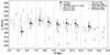 |
Fig. 6. Circular velocity curve obtained from the MCMC. Grey dashed lines have been plotted to indicate the position of each radial bin. In black (with circles) we show the circular velocities as obtained in this paper where the error bars correspond to the 16th and 84th percentile of the circular velocity posterior distribution in a particular bin. We adopted R0 = 8.277 kpc to convert the adimensional coordinate x into Galactocentric distance R. |
In Fig. 6, we compare our result to others from the literature. Our circular velocity curve is in agreement with the one estimated in Ablimit et al. (2020) using the 3D velocity vector method on ∼103 classical Cepheids. However, for R > 8 kpc, we obtain larger circular velocities than those calculated by the same authors but using the proper motions of ∼600 classical Cepheids. The former and latter samples have around 370 Cepheids in common and both results show that modelling assumptions and/or tracer samples can induce differences in the estimated circular velocities of at least 10%. We note that these changes are larger than the estimated uncertainties in this work, which are in the ≲3% level. Our error bars include statistical uncertainties, which are negligible owing to the large data sample. They further include uncertainties in the spatial-kinematic morphology of the tracer stars (scale radius of the density profile hR and of the velocity distribution hσ) and in the Sun’s galactocentric distance. Circular velocities show a mild sensitivity to hR, specially for values hR ≤ 2.5 kpc and, at least within the prior range explored in our analysis, hσ and circular velocity central values are independent. On the contrary, the adopted value of R0 strongly affects the final circular velocities and it is the main source of systematic uncertainties (from the ones studied in this analysis).
In addition, our estimated circular velocities are also compatible with those obtained in Eilers et al. (2019), Wang et al. (2022) and Zhou et al. (2023), due to our large uncertainties compared to those estimated in these articles. If we fixed the Sun’s galactocentric distance and total velocity in the azimuthal direction to the values adopted in the former article, namely R0 = 8.122 kpc and V⊙ = 245.8 km s−1, the estimated error bars on the circular velocities are reduced and our results are incompatible with Eilers et al. (2019) analysis at 1σ for our fiducial distance estimates (see Sect. 4.4 for a comparison using the circular velocity curve obtained with other distance estimates). This shows that R0 is the main source of uncertainty in the reconstruction of the circular velocity curve. Moreover, if for the fixed R0 case the prior range in the scale length hσ is increased by a factor of three, the results remain unchanged. In contrast, increasing the prior range in the scale length hR by the same factor, the median values decrease by less than 2% and the size of error bars remains roughly the same.
The circular velocity curve in Wang et al. (2022) was obtained by describing, by means of the radial axisymmetric Jeans equation, the dynamics of all Gaia DR3 stars within the region 160o < ℓ < 200° and |Z| < 3 kpc that have measured radial velocities. All stars are thus described by the same asymmetric drift. However, younger stars are expected to have a smaller asymmetric drift than an older population of stars. In fact, Kawata et al. (2019) estimated va(R0) = 0.28 ± 0.20 km s−1 using young classical Cepheids, whether we obtain, as expected, the central larger value va(R0) = 3 ± 7 km s−1 for older RGB stars. Figure 7 shows the asymmetric drift as a function of Galactocentric distance for R0 = 8.277 kpc. The asymmetric drift mildly increases with distance to the Galactic centre with a slope of 0.59 ± 0.12 km s−1 kpc−1.
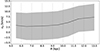 |
Fig. 7. Asymmetric drift profile. The black line shows the asymmetric drift correction in each radial bin and the shaded region depicts its propagated uncertainty. We note that the uncertainties are fully correlated between the bins. |
Our estimated value of the circular velocity at the Sun’s position, namely 233 ± 7 km s−1, is compared in Table 2 with other estimates from the literature. We found that the estimated gradient of the curve is extremely sensitive to the radial interval included in its inference. If we remove the first two radial bins where the circular velocities increase, the obtained value is −1.1 ± 0.3 km s−1 kpc−1, which points to a smooth decrease of the circular velocities with Galactocentric distances. If we rather include all radial bins, the estimated value of the slope is 0.4 ± 0.6 km s−1 kpc−1, which describes a flat circular velocity curve within the uncertainties. Mróz et al. (2019) and Eilers et al. (2019) included all radial intervals for the determination of the slope, and found decreasing slopes that do not agree with the latter value. This may point out to the presence of systematic biases in the distance estimations, as described in Sect. 4.4.
Circular velocity at the solar location vc(R0) as measured by different methods.
4.2. Smooth dark matter halo
In the region analysed in this article, mean radial velocities are < 5% of the azimuthal or rotational velocities. According to Chrobáková et al. (2020), when the ratio of radial to azimuthal velocities is smaller than 10%, circular velocities obtained through the radial axisymmetric and stationary Jeans equation provide an unbiased estimator for the centrifugal velocities that balance the averaged radial gravitational force. According to this result, our circular velocity curve then provides an unbiased estimation of the spherically averaged dynamical mass distribution within 14 kpc. Although this conclusion will be tested in an upcoming paper where we assess the effects of modelling assumptions, such as the axial symmetry condition, and the effect of Galactic substructure, using our current results we estimate that the DM mass is
![Mathematical equation: $$ \begin{aligned} \log _{10}\left[M_{\rm DM}(R < 14\,\mathrm{kpc})/{M_{\odot }}\right]= 11.2^{+2.0}_{-2.3}. \end{aligned} $$](/articles/aa/full_html/2023/08/aa46474-23/aa46474-23-eq27.gif) (9)
(9)
Furthermore, we find that the local spherically averaged DM density is
 (10)
(10)
These estimates were obtained by fitting the observed circular velocities to the velocities predicted by Newtonian gravity for the baryonic components (stellar bulge, disc and gas) and the DM halo. For each baryonic component we adopted a set of three-dimensional density profiles, originally compiled in Iocco et al. (2015). The stellar bulge mass is constrained by microlensing towards the Galactic centre and the stellar disc is normalised by the stellar surface density at the Sun’s position. We describe the DM distribution using a generalised Navarro-Frenk-White density profile Zhao (1996). We compare observed and predicted velocities using the Bayesian prescription presented in Karukes et al. (2019, 2020). The estimates provided are Bayesian model averages that include uncertainties in the Sun’s Galactocentric distance, the three-dimensional density profile of bulge and disc stars, and the stellar mass of the Galaxy.
We would like to highlight that our estimate of the local DM density is compatible, within 1σ uncertainties, with recent estimates of this quantity using the circular velocity curve method (Eilers et al. 2019; Mróz et al. 2019; de Salas et al. 2019; Lin & Li 2019; Karukes et al. 2019; Sofue 2020). In addition, it is compatible with local estimates using the vertical Jeans equation (Salomon et al. 2020; Guo et al. 2020; Nitschai et al. 2020) and with the most-recent local estimate using a novel machine learning approach by Lim et al. (2023). Thus reinforcing the conclusion about the spherical shape of the inner ∼ 15 kpc of the DM halo, obtained by modelling stellar streams (Koposov et al. 2010; Bowden et al. 2015) and the kinematics of halo stars Wegg et al. (2019).
4.3. The local standard of rest and the solar peculiar velocity
The total Galactocentric azimuthal velocity of the Sun can be used to derive the solar peculiar velocity when we incorporate knowledge about the circular velocity at its position. In particular, the total azimuthal velocity is often decomposed as
 (11)
(11)
where the last term is the Sun’s peculiar motion in the local standard of rest (LSR). The treatment of the solar velocity as shown in Eq. (11) assumes that the LSR moves in a circular orbit about the Galactic centre and therefore, it coincides with the rotational standard of rest (RSR) in which stars move on circular orbits in the azimuthally averaged gravitational potential. However, in recent years it has been shown that the stellar disc exhibits bulk motions at the kiloparsec scale (Bovy et al. 2015; Williams et al. 2013; Khanna et al. 2023). In the presence of these large scale streaming motions, the LSR, which is defined as the reference frame of a local population of stars with zero velocity dispersion, might not coincide with the RSR. Considering this, the total azimuthal velocity of the Sun can be decomposed as (Drimmel & Poggio 2018)
 (12)
(12)
where VLSR is the velocity of the LSR with respect to the RSR. This difference of velocity between the LSR and RSR might account for the discrepancy between locally-derived estimations of the Sun’s peculiar motion (i.e. using the Strömberg relation) and globally-measured values using a sample of tracers in a larger volume around the Sun. In fact, Bovy et al. (2012) concluded that the LSR itself might not be on a circular orbit and it is rotating VLSR ≈ 12 km s−1 faster than the actual RSR. This is in agreement with the recently reported value in Khanna et al. (2023) of ≈10 km s−1. On the other hand, Bland-Hawthorn & Gerhard (2016) estimated VLSR = 0 ± 15 km s−1.
Assuming V⊙,LSR = 12.24 km s−1 as measured in Schönrich et al. (2010) from the Hipparcos Catalogue, we obtain VLSR = 7 ± 7 km s−1. Our estimate is still statistically compatible with zero streaming motion, but nevertheless strengthens the hypothesis that a region around the Sun, with a characteristic length scale of 1 kpc, exhibits a bulk motion in the azimuthal direction of the order of 10 km s−1.
4.4. Cautionary tale about distances
Our study is based on GSP-Phot distances (Andrae et al. 2023), which have been shown to systematically underestimate the distance beyond 2 kpc from the Sun (Fouesneau et al. 2023). This bias is also shown in the left panel of Fig. 1, as the two-dimensional distribution of the estimated distance versus inverse parallax is not symmetric with respect to the 1:1 line, as expected from a Gaussian noise model for parallax measurements, but is more populated to the right of this line. Fouesneau et al. (2023) find that imposing a cut-off in the quality of the parallax measurement of ϖ/σϖ > 10 yields reliable heliocentric distances up to 10 kpc. And Andrae et al. (2023) point out that a strict parallax quality cut-off of ϖ/σϖ > 20 provides reliable distances. For our sample of RGB stars, the first cut-off eliminates the systematic underestimation of the GSP-Phot distances, although a slight overestimation of distances appears (see left panel of Fig. 1). For this reason, as our fiducial run, we adopted the last strict cut, which alleviates the mild overestimation. However, in this section we describe how our results would change if we had adopted the less stringent cut-off in parallax quality or rather used photogeo distances from Bailer-Jones et al. (2021) (hereinafter referred to as BJ distances).
A bias in distance estimates has a noticeable impact in the results of our analysis. In particular, underestimated distances lead to an overestimation of the circular velocity curve gradient, and thus to an underestimation of the DM content, and vice versa in the case of overestimated distances. We note that the bias in the estimated slope is more pronounced the greater the actual slope. In order to assess the effect of biased distances, we performed our MCMC analysis using four different distance estimates: BJ distances with a cut-off of ϖ/σϖ > 5 and ϖ/σϖ > 10, and GSP-Phot distances with ϖ/σϖ > 10 and ϖ/σϖ > 20. For each of these distance estimates, the top panel of Fig. 8 shows the resultant circular velocity curve while fixing the Sun’s galactocentric distance and total velocity in the azimuthal direction to the values adopted in Eilers et al. (2019), namely R0 = 8.122 kpc and V⊙ = 245.8 km s−1, and leaving hR and hσ free. The bottom panel of the same figure depicts circular velocities while letting R0 as an additional free parameter. From this figure, it is clear that the inclusion of uncertainties in R0 makes the four circular velocities compatible within uncertainties. Furthermore, as we increase the cut-off in the parallax quality from 5 to 10 for BJ distances, the declining of the curve becomes less steep, thus increasing the DM mass of the Galaxy. On the other hand, by increasing the cut-off from 10 to 20 for the GSP-Phot distances, we are alleviating the mild overestimation of distances and the positive gradient of the curves becomes shallower, reducing the DM mass. Table 3 summarises these results.
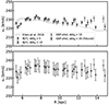 |
Fig. 8. Circular velocity curve for different distances estimates as explained in the main text. In the top panel, we show the results where fixing the Sun’s galactocentric distance to R0 = 8.122 kpc and leaving free the scale lengths of the radial spatial density and velocity dispersion of the tracer RGB sample. The orange band shows encompass the estimated circular velocity curve in Eilers et al. (2019) within 1σ. The results when additionally leaving R0 as a free parameter are shown in the bottom panel. |
Summary of the results when having R0, hR and hσ as free parameters and adopting different distance estimates.
5. Summary and conclusions
We estimated the circular velocity curve from 5 kpc to 14 kpc from the Galactic centre using 665 660 RGB stars that are approximately located in one quarter of the stellar disc with 6D phase-space information as measured by Gaia DR3, and GSP-Phot distance estimates. We determined the circular velocity curve by describing observed rotational velocities, in adimensional radial bins, as the difference between the circular velocity and the asymmetric drift. The latter given by the stationary and axisymmetric radial Jeans equations, under the further assumption of reflection symmetry above and below the Galactic plane. In the traditional approach, one simply plugs values into the Jeans equation. In our approach, by describing the observed rotational velocity as the circular velocity minus the asymmetric drift, we transformed the problem into an inference procedure. In particular, observed and model rotational velocities were fitted using a Bayesian inference approach that incorporates systematic and statistical uncertainties as nuisance parameters. This allowed us to propagate into the final results uncertainties of different nature. In particular, our relative uncertainties are ∼3% and, apart from the statistics, account for uncertainties in the Sun’s galactocentric distance (which is the main source of uncertainty) and uncertainties in the spatial-kinematic morphology of the stellar disc.
We studied the effect of biased distances on our results and showed, as expected, that underestimated distances lead to steeper (negative) slopes and thus to an underestimation of the dark matter content in the Galaxy. This may explain some recent findings of significantly declining circular velocity curves and, consequently, lower spherically averaged local DM densities than those purely local values obtained using stars in the Solar neighbourhood. Owing to the spherical shape of the DM halo in the inner ∼15 kpc of the Galaxy, these two sets of estimates should converge.
v⊙ is defined in Eq. (1).
By adopting an alternative Z0 value of 0 pc, the change in the central circular velocities is smaller than 1%.
To avoid confusion between uncertainties and the components of the velocity-dispersion tensor, we add the superscript to the latter as in Gaia Collaboration (2023).
https://github.com/HEP-KBFI/gaia-tools
Acknowledgments
We thank the referee for her/his constructive comments and for pointing out the biases in the distance estimates. This has undoubtedly opened up many avenues for further studies. The authors would like to thank A. Cuoco, G. Battaglia and E. Fernández Alvar for fuitful discussions and comments. This work was supported by the Estonian Research Council grants PRG1006, PSG700, PRG803, PSG864, MOBTP187, PRG780, MOBTT86 and by the European Regional Development Fund through the CoE program grant TK133. This research has made use of data from the European Space Agency (ESA) mission Gaia (https://www.cosmos.esa.int/gaia), processed by the Gaia Data Processing and Analysis Consortium (DPAC, https://www.cosmos.esa.int/web/gaia/dpac/consortium). Funding for the DPAC has been provided by national institutions, in particular the institutions participating in the Gaia Multilateral Agreement. The authors gratefully acknowledge the support of Nvidia, whose technology played a critical role in the success of this research. G.F.T. acknowledges support from the Agencia Estatal de Investigación del Ministerio de Ciencia en Innovacón (AEI-MICIN) under grant number CEX2019-000920-S and the AEI-MICIN under grant number PID2020-118778GB-I00/10.13039/501100011033
References
- Ablimit, I., Zhao, G., Flynn, C., & Bird, S. A. 2020, ApJ, 895, L12 [Google Scholar]
- Abuter, R., Amorim, A., Anugu, N., et al. 2018, A&A, 615, L15 [NASA ADS] [CrossRef] [EDP Sciences] [Google Scholar]
- Andrae, R., Fouesneau, M., Sordo, R., et al. 2023, A&A, 674, A27 [CrossRef] [EDP Sciences] [Google Scholar]
- Bailer-Jones, C. A. L., Rybizki, J., Fouesneau, M., Demleitner, M., & Andrae, R. 2021, AJ, 161, 147 [Google Scholar]
- Benito, M., Bernal, N., Bozorgnia, N., Calore, F., & Iocco, F. 2017, J. Cosmol. Astropart. Phys., 2017, 007 [CrossRef] [Google Scholar]
- Benito, M., Cuoco, A., & Iocco, F. 2019, J. Cosmol. Astropart. Phys., 2019, 033 [CrossRef] [Google Scholar]
- Binney, J., & Tremaine, S. 2008, Galactic Dynamics: Second Edition [Google Scholar]
- Bland-Hawthorn, J., & Gerhard, O. 2016, ARA&A, 54, 529 [Google Scholar]
- Bobylev, V. V. 2017, Astron. Lett., 43, 152 [NASA ADS] [CrossRef] [Google Scholar]
- Bovy, J., Allende Prieto, C., Beers, T. C., et al. 2012, ApJ, 759, 131 [NASA ADS] [CrossRef] [Google Scholar]
- Bovy, J., Bird, J. C., Pérez, A. E. G., et al. 2015, ApJ, 800, 83 [NASA ADS] [CrossRef] [Google Scholar]
- Bowden, A., Belokurov, V., & Evans, N. W. 2015, MNRAS, 449, 1391 [NASA ADS] [CrossRef] [Google Scholar]
- Chrobáková, Ž., López-Corredoira, M., Sylos Labini, F., Wang, H. F., & Nagy, R. 2020, A&A, 642, A95 [NASA ADS] [CrossRef] [EDP Sciences] [Google Scholar]
- de Salas, P. F., Malhan, K., Freese, K., Hattori, K., & Valluri, M. 2019, J. Cosmol. Astropart. Phys., 2019, 037 [Google Scholar]
- Do, T., Hees, A., Ghez, A., et al. 2019, Science, 365, 664 [Google Scholar]
- Drimmel, R., & Poggio, E. 2018, Res. Notes Am. Astron. Soc., 2, 210 [Google Scholar]
- Eilers, A.-C., Hogg, D. W., Rix, H.-W., & Ness, M. K. 2019, ApJ, 871, 120 [Google Scholar]
- Foreman-Mackey, D., Hogg, D. W., Lang, D., & Goodman, J. 2013, PASA, 125, 306 [CrossRef] [Google Scholar]
- Fouesneau, M., Frémat, Y., Andrae, R., et al. 2023, A&A, 674, A28 [NASA ADS] [CrossRef] [EDP Sciences] [Google Scholar]
- Gaia Collaboration (Prusti, T., et al.) 2016, A&A, 595, A1 [NASA ADS] [CrossRef] [EDP Sciences] [Google Scholar]
- Gaia Collaboration (Katz, D., et al.) 2018, A&A, 616, A11 [NASA ADS] [CrossRef] [EDP Sciences] [Google Scholar]
- Gaia Collaboration (Drimmel, R., et al.) 2023, A&A, 674, A37 [CrossRef] [EDP Sciences] [Google Scholar]
- GRAVITY Collaboration (Abuter, R., et al.) 2019, A&A, 625, L10 [NASA ADS] [CrossRef] [EDP Sciences] [Google Scholar]
- GRAVITY Collaboration (Abuter, R., et al.) 2020, A&A, 636, L5 [NASA ADS] [CrossRef] [EDP Sciences] [Google Scholar]
- GRAVITY Collaboration (Abuter, R., et al.) 2021, A&A, 647, A59 [NASA ADS] [CrossRef] [EDP Sciences] [Google Scholar]
- GRAVITY Collaboration (Abuter, R., et al.) 2022, A&A, 657, L12 [NASA ADS] [CrossRef] [Google Scholar]
- Guo, R., Liu, C., Mao, S., et al. 2020, MNRAS, 495, 4828 [Google Scholar]
- Harris, C. R., Millman, K. J., van der Walt, S. J., et al. 2020, Nature, 585, 357 [NASA ADS] [CrossRef] [Google Scholar]
- Helmi, A., Babusiaux, C., Koppelman, H. H., et al. 2018, Nature, 563, 85 [Google Scholar]
- Hobbs, D., Lindegren, L., Bastian, U., et al. 2018, Gaia DR2 documentation Chapter 3: Astrometry [Google Scholar]
- Huang, Y., Liu, X.-W., Yuan, H.-B., et al. 2016, MNRAS, 463, 2623 [CrossRef] [Google Scholar]
- Iocco, F., Pato, M., & Bertone, G. 2015, Nat. Phys., 11, 245 [NASA ADS] [CrossRef] [Google Scholar]
- Johnson, D. R. H., & Soderblom, D. R. 1987, AJ, 93, 864 [Google Scholar]
- Jurić, M., Ivezić, Ž., Brooks, A., et al. 2008, ApJ, 673, 864 [Google Scholar]
- Karukes, E. V., Benito, M., Iocco, F., Trotta, R., & Geringer-Sameth, A. 2019, J. Cosmol. Astropart. Phys., 2019, 046 [Google Scholar]
- Karukes, E. V., Benito, M., Iocco, F., Trotta, R., & Geringer-Sameth, A. 2020, J. Cosmol. Astropart. Phys., 2020, 033 [CrossRef] [Google Scholar]
- Kawata, D., Bovy, J., Matsunaga, N., & Baba, J. 2019, MNRAS, 482, 40 [NASA ADS] [CrossRef] [Google Scholar]
- Khanna, S., Sharma, S., Bland-Hawthorn, J., & Hayden, M. 2023, MNRAS, 520, 5002 [CrossRef] [Google Scholar]
- Kipper, R., Tenjes, P., Tihhonova, O., Tamm, A., & Tempel, E. 2016, MNRAS, 460, 2720 [NASA ADS] [CrossRef] [Google Scholar]
- Kipper, R., Tenjes, P., Tempel, E., & de Propris, R. 2021, MNRAS, 506, 5559 [NASA ADS] [CrossRef] [Google Scholar]
- Koposov, S. E., Rix, H.-W., & Hogg, D. W. 2010, ApJ, 712, 260 [Google Scholar]
- Kuzmin, G. G. 2022, ArXiv e-prints [arXiv:2201.04136] [Google Scholar]
- Leung, H. W., Bovy, J., Mackereth, J. T., et al. 2022, MNRAS, 519, 948 [CrossRef] [Google Scholar]
- Lim, S. H., Putney, E., Buckley, M. R., & Shih, D. 2023, ArXiv e-prints [arXiv:2305.13358] [Google Scholar]
- Lin, H.-N., & Li, X. 2019, MNRAS, 487, 5679 [CrossRef] [Google Scholar]
- Malkin, Z. M. 2013, Astron. Rep., 57, 128 [NASA ADS] [CrossRef] [Google Scholar]
- Mróz, P., Udalski, A., Skowron, D. M., et al. 2019, ApJ, 870, L10 [Google Scholar]
- Nitschai, M. S., Cappellari, M., & Neumayer, N. 2020, MNRAS, 494, 6001 [Google Scholar]
- Okuta, R., Unno, Y., Nishino, D., Hido, S., & Loomis, C. 2017, in Proceedings of Workshop on Machine Learning Systems (LearningSys) in The Thirty-first Annual Conference on Neural Information Processing Systems (NIPS) [Google Scholar]
- Reid, M. J., & Brunthaler, A. 2020, ApJ, 892, 39 [Google Scholar]
- Rybizki, J., Green, G. M., Rix, H.-W., et al. 2022, MNRAS, 510, 2597 [NASA ADS] [CrossRef] [Google Scholar]
- Salomon, J.-B., Bienaymé, O., Reylé, C., Robin, A. C., & Famaey, B. 2020, A&A, 643, A75 [EDP Sciences] [Google Scholar]
- Schönrich, R., Binney, J., & Dehnen, W. 2010, MNRAS, 403, 1829 [NASA ADS] [CrossRef] [Google Scholar]
- Sofue, Y. 2020, Galaxies, 8, 37 [Google Scholar]
- Tempel, E., & Tenjes, P. 2006, MNRAS, 371, 1269 [NASA ADS] [CrossRef] [Google Scholar]
- Thomas, G. F., Laporte, C. F. P., McConnachie, A. W., et al. 2019, MNRAS, 483, 3119 [Google Scholar]
- Wang, H. F., Chrobáková, Ž., López-Corredoira, M., & Labini, F. S. 2022, ApJ, 942, 12 [Google Scholar]
- Wegg, C., Gerhard, O., & Bieth, M. 2019, MNRAS, 485, 3296 [NASA ADS] [CrossRef] [Google Scholar]
- Williams, M. E. K., Steinmetz, M., Binney, J., et al. 2013, MNRAS, 436, 101 [Google Scholar]
- Zhao, H. 1996, MNRAS, 278, 488 [Google Scholar]
- Zhou, Y., Li, X., Huang, Y., & Zhang, H. 2023, ApJ, 946, 73 [CrossRef] [Google Scholar]
Appendix A: MCMC results
Figure A.1 shows the marginalised two-dimensional and one-dimensional posterior distributions for three different MCMC runs: first, (R0, hR, hσ) are free nuisance parameters (black), second, (hR, hσ) are not fixed and R0 is fixed to the value R0 = 8.122 kpc (red) and finally, the output of the MCMC when all nuisance parameters are fixed to the values R0 = 8.277 kpc, hR = 3 kpc, hσ = 21 kpc.
 |
Fig. A.1. One and two-dimensional marginalised posterior distributions of the circular velocity. The figure shows distributions from three different parameter setups: all nuissance parameters free (black), only scale parameters free (red), all nuissance parameters fixed (blue), see text for more details. The contours delimit regions of 2-σ probability and the best fit circular velocity of the black posteriors is demarked with horisontal and vertical lines. The diagonal contains the normalised 1D posteriors of the circular velocities from the three different runs. |
For the first run (i.e. R0, hR and hσ are free parameters), the movement of circular velocities is driven by changes in R0. Since we are not considering strong priors on R0, a strong positive correlation between this parameter and the circular velocities is observed. The circular velocity curve is sensitive to the Sun’s Galactocentric distance R0 (Benito et al. 2019), nonetheless, R0 is constrained in the literature much better by different types of analysis than the circular velocities (see Malkin 2013 for a review of techniques). Therefore, we do not aim to restrict R0, but to assess the impact of its uncertain value on the circular velocity curve. For this reason, we adopt as a prior a uniform distribution that encompasses the most recent determinations of R0 within 2σ uncertainties. This is a conservative approach that does not favour any particular estimate. We would like to also emphasise that the actual value of R0 may be troublesome. For example, the LMC is causing differences in reflex motion in distinct parts of the Galaxy causing the definition of centre to be vague or we do not know to what extent the different definitions of centre (e.g. local isopotential curve, SMBH position) affect estimations via the Jeans equations. One of the results of our analysis is that, given the scatter in the most recent determination of R0, this parameter represents the main source of uncertainty in the calculation of circular velocities in radial bins.
On the contrary, circular velocities show a mild sensitivity to hR and hσ. Neither of these scale lengths can be constrained by our analysis and are simply treated as nuisance parameters whose prior range is defined by observational determinations (see e.g. Eilers et al. 2019 and references therein).
All Tables
Circular velocity at the solar location vc(R0) as measured by different methods.
Summary of the results when having R0, hR and hσ as free parameters and adopting different distance estimates.
All Figures
|
Fig. 1. Bias in different distance estimates. Left: GSP-Phot heliocentric distances as a function of parallax inverse. The colour bar shows the mean parallax quality inside each pixel. The quality cut used in this paper corresponds to log10(ϖ/σϖ) > 1.301. Right: same but for photogeo heliocentric distances by Bailer-Jones et al. (2021). |
| In the text | |
|
Fig. 2. Spatial distribution of the final red giants sample. Left: distribution in the Galactic longitude (ℓ) and latitude (b) plane. The colour bar shows the number density of stars per pixel. Each pixel has a size of 1 degree in both latitude and longitude. Right: same but projected into the Galactic plane. Each pixel has a size of 0.05 kpc and 0.06 kpc in the x and y coordinates, respectively. In this figure, the Galactic centre is located at (0, 0), the Sun is located at ( − 8.277, 0) and the rotation of the Galaxy is clockwise. We added dashed, black circles at 5 kpc, R0 = 8.277 kpc, 12 kpc and 14 kpc to ease visualisation. For the transformation to Galactocentric coordinades, we adopt R0 = 8.277 kpc, z0 = 25 pc and v⊙ = (11.1, 251.5, 8.59) km s−1. |
| In the text | |
|
Fig. 3. Distribution of the mean observed rotational velocity vϕ inside x–y pixels for our final sample of RGB stars (left). The size of the bin is 150 pc in both x and y coordinates, respectively. We added dashed, black circles at 5 kpc, R0 = 8.277 kpc, 12 and 14 kpc to ease visualisation. Square root of the radial and azimuthal diagonal components of the velocity dispersion tensor in radial bins of 1 kpc (right). |
| In the text | |
|
Fig. 4. Mean azimuthal (left) and radial (right) velocities as a function of Galactocentric distance R. As in Fig. 3, errorbars are calculated via bootstrap (see text for details). |
| In the text | |
|
Fig. 5. Distribution of vϕ inside the last radial bin where the distribution of values deviates most from a Gaussian distribution (orange) and a randomly selected bin (blue). The dashed lines depict the best-fitted Gaussian of the rotational velocity inside each particular bin. |
| In the text | |
|
Fig. 6. Circular velocity curve obtained from the MCMC. Grey dashed lines have been plotted to indicate the position of each radial bin. In black (with circles) we show the circular velocities as obtained in this paper where the error bars correspond to the 16th and 84th percentile of the circular velocity posterior distribution in a particular bin. We adopted R0 = 8.277 kpc to convert the adimensional coordinate x into Galactocentric distance R. |
| In the text | |
|
Fig. 7. Asymmetric drift profile. The black line shows the asymmetric drift correction in each radial bin and the shaded region depicts its propagated uncertainty. We note that the uncertainties are fully correlated between the bins. |
| In the text | |
|
Fig. 8. Circular velocity curve for different distances estimates as explained in the main text. In the top panel, we show the results where fixing the Sun’s galactocentric distance to R0 = 8.122 kpc and leaving free the scale lengths of the radial spatial density and velocity dispersion of the tracer RGB sample. The orange band shows encompass the estimated circular velocity curve in Eilers et al. (2019) within 1σ. The results when additionally leaving R0 as a free parameter are shown in the bottom panel. |
| In the text | |
|
Fig. A.1. One and two-dimensional marginalised posterior distributions of the circular velocity. The figure shows distributions from three different parameter setups: all nuissance parameters free (black), only scale parameters free (red), all nuissance parameters fixed (blue), see text for more details. The contours delimit regions of 2-σ probability and the best fit circular velocity of the black posteriors is demarked with horisontal and vertical lines. The diagonal contains the normalised 1D posteriors of the circular velocities from the three different runs. |
| In the text | |
Current usage metrics show cumulative count of Article Views (full-text article views including HTML views, PDF and ePub downloads, according to the available data) and Abstracts Views on Vision4Press platform.
Data correspond to usage on the plateform after 2015. The current usage metrics is available 48-96 hours after online publication and is updated daily on week days.
Initial download of the metrics may take a while.