© The Authors 2023

1 Introduction

Recent work suggests that the study of transit light curves of extra-solar planets may provide information on their shape, which is linked to the value of the second-degree fluid Love number k₂ (see e.g. Carter & Winn 2010; Correia 2014; Kellermann et al. 2018; Hellard et al. 2018, 2019; Akinsanmi et al. 2019; Barros et al. 2022). According to Padovan et al. (2018), estimates of k₂ for extra-solar planets may become available in the near future, in view of the expected improvements in the observational facilities and the increasing amount of data. For a fluid-like giant planet k₂ is sensitive to the density layering (e.g. Ragozzine & Wolf 2009; Kramm et al. 2011; Padovan et al. 2018), which means that transit observations may potentially provide, in the near future, new constraints on the internal structure of exoplanets. This will have important implications on our knowledge of the internal planetary dynamics and the formation history (e.g. Kramm et al. 2011).

Using a matrix-propagator approach borrowed from global geodynamics, Padovan et al. (2018) compute numerically the fluid k₂ Love number for planetary models of increasing complexity, ranging from two-layer to multi-layered structures. Padovan and colleagues find that the normalised mean polar moment of inertia of a planet and k₂ show a similar sensitivity to the mass concentration (i.e. they both decrease with increasing mass concentration at depth), thus supporting the results of Kramm et al. (2011). The theory developed by Padovan et al. (2018) is strictly suitable for close-in, tidally locked gaseous extra-solar planets, for which the first experimental determinations of k₂ are expected due to their large size and flattening (Hellard et al. 2018). The N-k₂ relation has never been explored for Earths or super-Earths that include layers of finite rigidity and are less deformable than gaseous planets (Hellard et al. 2019).

In this work we delve further into the N-k₂ relation for a fluid multi-layered extra-solar planet, with the purpose of refining the implicit approximation of Padovan et al. (2018), namely N ≈ k₂. Following these authors, we first adopt a basic two-layer planet, and taking advantage of the closed-form expression for k₂ first published by Ragazzo (2020), we show that an extremely simple power law (rule of thumb, or ROT) better captures the relation between N and k₂. Second, by running a Monte Carlo simulation, we show that for multi-layered models the rule of thumb determines an upper limit for N for a given hypothetically observed k₂ value. In both cases the rules obtained are superior to the Radau-Darwin formula (e.g. Cook 1980).

This paper is organised as follows. In Sect. 2 we recall some basic analytical results regarding the k₂ Love number and N for a two-layer fluid planet. In Sect. 3 we discuss a possible approximate relation between N and k₂ for a two-layer model, and test its validity for multi-layered planets through a suite of numerical experiments. Finally, we draw our conclusions in Sect. 4.

2 Analytical results for a fluid two-layer planet

2.1 k₂ Love number

In the special case of a fluid planet, k₂ only depends on the density profile. The equilibrium equations reduce to a linear second-order differential equation for the perturbed gravitational potential φ that reads $$\phi ″+\frac{2}{r}\phi \prime -\left(\frac{n\left(n+1\right)}{r^2}+\frac{4\pi G}{g_0}{\rho }_0^{\prime }\right)\phi =0,$$(1)

where the prime denotes the derivative with respect to radius r, n is the harmonic degree, g₀(r) is gravity acceleration, and ρ₀(r) is density (Wu & Peltier 1982)¹. Assuming layers of constant density (i.e. ${\rho }^{\prime }{}_0=0$), Eq. (1) allows for a closed-form solution in terms of powers of r. For non-fluid planets that include elastic or visco-elastic layers, a full set of six spheroidal equilibrium equations must be solved, since in this case φ is coupled with the tide-induced displacements (see e.g. Wu & Peltier 1982; Melini et al. 2022).

Denoting the radius of the inner layer (the core) and its density respectively as r_c and ρ_c, and the corresponding quantities for the outer layer (the mantle) as r_m and ρ_m, with the aid of the Mathematical© (Wolfram Research 2010) symbolic manipulator for n = 2 we find $${\tilde{k}}_2=2\frac{5+\alpha \left(5\alpha z^8+8\left(1-\alpha \right)z^5+3\alpha -8\right)}{10+\alpha \left(9z^5\left(\alpha -1\right)+5z^3\left(5-3\alpha \right)+6\alpha -16\right)},$$(2)

where ${\tilde{k}}_2$ is the normalised Love number $${\tilde{k}}_2=\frac{k_2}{k_{2h}}$$(3)

and $$k_{2h}=\frac{3}{2}$$(4)

is the Love number for a homogeneous planet (see e.g. Munk & MacDonald 1975). In Eq. (2) we have introduced the non-dimensional core radius $$z=\frac{r_{\text{c}}}{r_{\text{m}}},$$(5)

with 0 ≤ z ≤ 1, and the ratio $$\alpha =\frac{{\rho }_{\text{c}}-{\rho }_{\text{m}}}{{\rho }_{\text{c}}}.$$(6)

We note that for a gravitationally stable planet (ρ_c ≥ ρ_m) we have 0 ≤ α ≤ 1. The value α = 1 corresponds to the limit case of a mass-less mantle (ρ_m = 0), whereas for a homogeneous planet (ρ_m = ρ_c), the value is α = 0.

Since the planet is fluid and inviscid, vertical displacement is interpreted as the displacement of equipotential surfaces so that the vertical Love number is h₂ = 1 + k₂. As the tangential displacement is undetermined within a perfect fluid, the l₂ Love number is undefined. Further, $k^{\prime }{}_2=k_2-h_2$, where k₂ is the loading Love number for gravitational potential (Molodensky 1977). Hence, $k^{\prime }{}_2+1=0$, which manifests a condition of perfect isostatic equilibrium (see e.g. Munk & MacDonald 1975). By symbolic manipulation, it is also possible to obtain a general closed-form expression for k_n at harmonic degrees n ≥ 2, which is reported, probably for the first time, in Appendix A. It is worth noting that, although in Eq. (2) ${\tilde{k}}_2$ is written in terms of α and z, it depends implicitly on the four parameters defining the model (namely, r_c, r_m, ρ_c, and ρ_m). Thus, even assuming that the size of a hypothetical extra-solar planet is known and that we dispose of an observed value of ${\tilde{k}}_2$, it is impossible to determine the remaining three quantities unambiguously.

As far as we know, for the two-layer model, the explicit form of ${\tilde{k}}_2$ was first published by Ragazzo (2020). It is easily verified that our Eq. (2) is equivalent to his Eqs. (2.40) and (2.41), taking into account that he defines α as ρ_m/ρ_c. Although Padovan et al. (2018) did not provide the explicit form for k₂, we have verified that Eq. (2) can be obtained through symbolic manipulation from their analytical propagators, and that it is also consistent, to a very high numerical precision, with the output from the Python codes that they have made available. Furthermore, by symbolic manipulation, we have verified that Eq. (2) is also confirmed taking the limit of vanishing frequency when the full set of six equilibrium equations for a general viscoelastic layered body are algebraically solved. A fully numerical computation using the Love numbers calculator ALMA³ of Melini et al. (2022) also confirms Eq. (2) to a very high precision.

As expected, the well-known result ${\tilde{k}}_2=1$, which is valid for the Kelvin sphere (Thomson 1863), is retrieved from Eq. (2) whenever one of the three limits $\alpha \mapsto 0$, $z\mapsto 0$ and $z\mapsto 1$ are taken. The smallest possible value of k₂ is met in the extreme condition of a point-like mass concentration at the planet centre (Roche model, see Roche 1873). With ρ_m ≪ ρ_c (hence $\alpha \mapsto 1$) and $z\mapsto 0$, Eq. (2) gives $k_2\mapsto 0$, in agreement with Padovan et al. (2018). In Fig. 1a the normalised Love number ${\tilde{k}}_2$ is shown as a function of α and z for the two-layer model, according to Eq. (2). It is apparent that, for a given α value, the same value of ${\tilde{k}}_2$ may be obtained for two distinct values of z. On the contrary, for a given z, knowledge of ${\tilde{k}}_2$ would determine α unequivocally. However, due to the definition of this parameter (Eq. (6)), knowledge of α would not suffice to determine the layer densities.

2.2 Mean polar moment of inertia

Following Ragozzine & Wolf (2009), Hellard et al. (2019), Kramm et al. (2011), and Padovan et al. (2018), here we pursue the idea that k₂ is a useful indicator of the mass concentration at depth inside a planet. It is well known that the radial density distribution is characterised by the normalised polar moment of inertia $$N=\frac{C}{M{R}^2},$$(7)

where C is the polar moment of inertia, M is the mass of the body, and R is the mean radius (see e.g. Hubbard 1984). The higher the mass concentration at depth, the smaller N is. By its own definition, N vanishes in the case of a point-like mass, while for a homogeneous sphere (e.g. Cook 1980) it attains the well-known value $$N_h=\frac{2}{5}.$$(8)

By defining $$\tilde{N}=\frac{N}{N_h},$$(9)

for a two-layer planet simple algebra provides $$\tilde{N}=\frac{1+\alpha \left(z^5-1\right)}{1+\alpha \left(z^3-1\right)},$$(10)

showing that Ñ and ${\tilde{k}}_2$ depend on the same parameters α and z, but in different combinations (see Eq. (2)), which suggests that establishing the $\tilde{N}-{\tilde{k}}_2$ relation may be not straightforward.

We further note that, in analogy with ${\tilde{k}}_2$, knowledge of Ñ would not allow us to invert Eq. (10) for α and z unequivocally (hence for the four model parameters r_c, r_m, ρ_c, and ρ_m), unless further constraints are invoked. Based on Eq. (10), in Fig. 1b the ratio Ñ is shown as a function of the parameters α and z. As noted for ${\tilde{k}}_2$ in Fig. 1a, for a given value of α the same Ñ can be obtained for two distinct values of z, while for a given z knowledge of Ñ would determine α unequivocally.

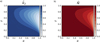Fig. 1 Contour plots showing ${\tilde{k}}_2$ (a) and Ñ (b) as a function of parameters α and z for a two-layer fluid planet, according to Eqs. (2) and (10), respectively. Since these variables are normalised to the values attained in the case of a homogeneous planet, they both range in the interval (0, 1).

3 Relation between the moment of inertia and the k₂ fluid Love number

3.1 Two-layer models

Padovan et al. (2018) establish a method for the evaluation of ${\tilde{k}}_2$ for a general fluid planet, based on the propagator technique often employed in geodynamics (e.g. Wu & Peltier 1982). Following the work of Kramm et al. (2011), they show that for a planet with two constant density fluid layers, Ñ and ${\tilde{k}}_2$ are directly correlated, both decreasing with increasing mass concentration at depth. However, Padovan et al. (2018) do not explicitly propose a general relation between these two quantities, which they suggest for particular planetary models characterised by a specific mass, size, and density (see their Fig. 3).

On the one hand, by comparing Figs. 1a with 1b it is apparent that, for our two-layer model, functions ${\tilde{k}}_2$ and Ñ have broadly similar shapes in the (α, z) plane, immediately suggesting a straightforward linear relation $\tilde{N}\simeq {\tilde{k}}_2$. This relation is implicitly proposed by Padovan et al. (2018) and would be exact for a uniform sphere. On the other hand, if we limit ourselves to an inspection of the analytical expressions (2) and (10), it is not easy to guess whether an exact $\tilde{N}\text{-}{\tilde{k}}_2$ relation may exist in analytical form. A priori, for a non-homogeneous planet this relation might be non-univalent, with more Ñ values corresponding to a given ${\tilde{k}}_2$ and vice versa.

After some symbolic manipulations, we verified that solving Eq. (10) for α and substituting into Eq. (2) would not provide insightful results. This suggests that an exact relation $\tilde{N}=\tilde{N}\left({\tilde{k}}_2\right)$ not involving α and z explicitly and valid for all values of these parameters can almost certainly be ruled out. Nevertheless, simple relations of partial validity could exist in some limiting cases where α or z take special values. 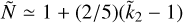For example, it is easy to show for small core bodies ($z\mapsto 0$) that $\tilde{N}\simeq 1+\left(2/5\right)\left({\tilde{k}}_2-1\right)$, which holds for all values of α and still implies that mass concentration at depth increases for decreasing ${\tilde{k}}_2$. Along the same lines, we note that for $\alpha \mapsto 1$, corresponding to case of a dense core surrounded by a light mantle, Eq. (10) gives Ñ ≃ z²; and since from Eq. (2) ${\tilde{k}}_2\simeq z^5$, by eliminating z we obtain a simple approximate power-law relation $\tilde{N}\simeq {\tilde{k}}_2^{0.4}$. We note that this last relation is actually an exact result for a homogeneous sphere surrounded by an hypothetical zero-density mantle, and can be obtained analytically by re-scaling the results for a Maclaurin spheroid (Hubbard 2013) of radius a to the outer radius r > a of the mass-less envelope (Hubbard 2023, priv. comm.).

The approximate $\tilde{N}\text{-}{\tilde{k}}_2$ relations discussed above are only valid for specific ranges of α and z. Certainly, a straightforward linear relation captures the broad similitude of the diagrams in Figs. 1a and 1b, but the solution may be too simplistic. Here, we seek a more general rule of thumb providing, within a certain level of approximation, a relation between Ñ and ${\tilde{k}}_2$ over all the points of the (α, z) plane. To quantify the error associated with a given ROT (e.g. ${\tilde{k}}_2$), we introduce the non-dimensional root mean square $$\text{RMS\hspace{0.17em}=\hspace{0.17em}}\sqrt{{\displaystyle {\int }_0^1{\displaystyle {\int }_0^1{\left[\tilde{N}-{\tilde{N}}_{\text{ROT}}\left({\tilde{k}}_2\right)\right]}^2\text{\hspace{0.17em}d}\alpha \text{\hspace{0.17em}d}z}}},$$(11)

where the double integral is evaluated numerically by standard methods.

First, we assume a direct proportionality $$\tilde{N}=c{\tilde{k}}_2,$$(12)

where c > 0 is a constant. Figure 2a shows, as a function of c, the RMS obtained with 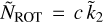${\tilde{N}}_{\text{ROT}}=c{\tilde{k}}_2$. The minimum RMS (close to 0.1168) is obtained for c ≈ 1.08, suggesting that the approximation $\tilde{N}\simeq {\tilde{k}}_2$ proposed by Padovan et al. (2018), and corresponding to c = 1, is indeed close to the best possible linear ROT.

Next, we consider a power-law relation $$\tilde{N}={\tilde{k}}_2^E,$$(13)

where E > 0 is an adjustable exponent. In Fig. 2b we show, as a function of E, the RMS corresponding to ${\tilde{N}}_{\text{ROT}}={\tilde{k}}_2^E$.It is apparent that the RMS is minimised for an exponent E ≈ 0.42, close to the value of 0.4 found analytically for a zero-density mantle. The corresponding minimum RMS value is ≈0.0082. These findings suggest that the relation $$\tilde{N}\approx {\tilde{k}}_2^{0.4}$$(14)

represents a simple and valid ROT expressing the link between Ñ and ${\tilde{k}}_2$ for a two-layer, fluid, stably layered planet characterised by arbitrary parameters α and z.

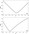Fig. 2 Non-dimensional RMS, evaluated according to Eq. (11), for a linear ROT $\tilde{N}\approx c{\tilde{k}}_2$ (frame a) and for a power-law ROT $\tilde{N}\approx {\tilde{k}}_2^E$ (b), as a function of the parameters c and E, respectively. Integrals in Eq. (11) have been evaluated numerically by the dblquad function included in the SciPy library (Virtanen et al. 2020).

3.2 Arbitrarily layered models

We have limited our attention to four-parameter models composed of two distinct fluid layers. To fully assess the validity of the ROT (Eq. (14)), it is now important to consider the case of a planetary structure consisting of an arbitrary number L of homogeneous layers.

Due to the model complexity, in this general case an analytical expressions for ${\tilde{k}}_2$ is not available; however, it is possible to evaluate ${\tilde{k}}_2$ numerically, for instance following the propagator method outlined by Padovan et al. (2018) or employing numerical Love number calculators such as ALMA (Melini et al. 2022). Conversely, an analytical expression for the normalised moment of inertia Ñ is easily obtained, also in the general case of an L-layer planet, and it reads $$\tilde{N}=\frac{{\displaystyle \sum _{i=1}^L\left(1-{\alpha }_i\right)\left(z_i^5-z_{i-1}^5\right)}}{{\displaystyle \sum _{i=1}^L\left(1-{\alpha }_i\right)\left(z_i^3-z_{i-1}^3\right)}},$$(15)

where z_i = r_i/r_m is the normalised radius of the outer boundary of the ith layer (z₀ ≡ 0) and $${\alpha }_i=\frac{{\rho }_1-{\rho }_i}{{\rho }_1},$$(16)

where ρ_i is the density of the i-th layer. By definition, z₁ ≤ … ≤ z_L = 1, while gravitational stability imposes ρ₁ ≤ … ≤ ρ_L so that 1 ≥ α_L ≥ … ≥ α₁ = 0. It is easily shown that, for L = 2, that Eq. (15) reduces to Eq. (10) with α ≡ α₂ and z ≡ z₁.

To test whether the ROT (Eq. (14)) can be of practical use also for general planetary structures, we generated an ensemble of 5 × 10⁵ models with a number of layers variable between L = 2 and L = 10, all characterised by a gravitationally stable density profile. For each of the planetary structures so obtained, we computed Ñ according to Eq. (15) and ${\tilde{k}}_2$ with the numerical codes made available by Padovan et al. (2018). The corresponding values of Ñ and ${\tilde{k}}_2$ are shown in Fig. 3 as grey dots.

For a given hypothetically observed ${\tilde{k}}_2$ value, the corresponding value of Ñ is clearly not unique. Rather, Ñ ranges within an interval, defined by the cloud of points whose width represents the uncertainty associated with the degree of mass concentration at depth. It is apparent that the maximum relative uncertainty on Ñ (up to ~50%) occurs for ${\tilde{k}}_2$ values ≲0.2 and that, for ${\tilde{k}}_2$ exceeding ≈0.5, the Ñ value is well constrained (to within ≈10%). This does not imply that the density profile of the planet is actually constrained, since Eq. (15) cannot be inverted for α_i and Z_i unequivocally without introducing further assumptions. The solid red line in Fig. 3 represents the ROT Eq. (14), obtained in the context of the two-layer model in Sect. 2.1. It is apparent that the ROT also remains valid in the general case of a L-layer planetary model and, for ${\tilde{k}}_2\gtrsim 0.5$, it provides a good estimate of Ñ once ${\tilde{k}}_2$ is known. For smaller values of ${\tilde{k}}_2$, the ROT represents an upper bound to the normalised moment of inertia: $$\tilde{N}\lesssim {\tilde{k}}_2^{0.4}.$$(17)

In the context of planetary structure modelling, the polytrope of unit index (Chandrasekhar & Milne 1933) has aparticularrel-evance. This simplified model resembles the interior barotrope of a hydrogen-rich planet in the Jovian mass range and, by virtue of its linear relation between mass density and gravitational potential, it allows the derivation of exact results useful for calibrating numerical solutions. Hubbard (1975) obtained analytical expressions of the moment of inertia and of the k₂ fluid Love numbers for a polytrope of index one (blue dot in Fig. 3). More recently, Wahl et al. (2020) modelled the equilibrium tidal response of Jupiter through the concentric Maclaurin spheroid method; their results in the non-rotating limit are also shown in Fig. 3 (green triangle). It is evident that the ROT is in excellent agreement for these two particular cases.

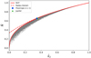Fig. 3 Fluid Love number ${\tilde{k}}_2$ and normalised moment of inertia Ñ for a random ensemble of 5 × 105 models with a number of layers 2 ≤ L ≤ 10. The solid red line shows the ROT $\tilde{N}={\tilde{k}}_2^{0.4}$. The dashed red line represents the Radau-Darwin (RD) formula (e.g. Cook 1980; Padovan et al. 2018; Ragazzo 2020). The RD formula is exact for a homogeneous body, but it constitutes an approximation for layered planets (Kramm et al. 2011; Padovan et al. 2018). The ROT and RD formulas match for ${\tilde{k}}_2\gtrsim 0.3$; for smaller values, our ROT represents a more rigorous upper limit to Ñ. The blue dot corresponds to values of ${\tilde{k}}_2$ and Ñ for a polytrope of index one, while the green triangle corresponds to the results by Wahl et al. (2020) for the equilibrium tidal response of Jupiter.

4 Conclusions

In this work we have re-explored the relation between the Love number ${\tilde{k}}_2$ of a fluid extra-solar planet and its mean polar moment of inertia Ñ. This relation would allow, in principle, an indirect inference of constraints on the internal mass distribution on the basis of an observational determination of ${\tilde{k}}_2$. However, we note that for a quantitative application of our results to real exoplanets, rotational effects and non-linear responses to rotational and tidal terms should be also considered (see e.g. Wahl et al. 2017, 2020).

We can draw two main conclusions. First, for a a hypothetical planet consisting of two homogeneous fluid layers, using the exact propagators method, we confirm that a relatively smooth analytical expressions of ${\tilde{k}}_2$ can be found. However, this expression does not allow us to establish a unique analytical relation between ${\tilde{k}}_2$ and Ñ except for some particular ranges of the model parameters. By investigating some approximate relations, for the first time we have determined the rule of thumb $\tilde{N}={\tilde{k}}_2^{0.4}$, which provides a good estimate of Ñ as a function of ${\tilde{k}}_2$ over the whole range of possible two-layer models. Second, using a Monte Carlo approach, we have explored the validity of our ROT in the general case of gravitationally stable planetary models with an arbitrarily large number of homogeneous layers. We find that the ROT provides an upper limit to the possible range of mean moment of inertia corresponding to a given value of ${\tilde{k}}_2$, and the distribution of downward departures from ROT increases as ${\tilde{k}}_2\mapsto 0$. In addition, the ROT is in good agreement with analytical results for a fluid polytrope body of unit index and with a realistic non-rotating model of the tidal deformation of Jupiter. Remarkably, our simulations show, especially for small values of k₂, that the ROT is more accurate than the celebrated Radau-Darwin (RD) formula.

Acknowledgements

We thank Bill Hubbard for his insightful review that greatly helped to improve the original manuscript. We are indebted to Roberto Casadio for discussion and to Leonardo Testi and Andrea Cimatti for encouragement. We also thank Nicola Tosi for advice. A.C. and G.S. are supported by a “RFO” DIFA grant.

Appendix A Analytical expression of k_n for a two-layer fluid model

Here we give an analytical expression for the tidal Love number of degree n ≥ 2 for a fluid two-layer extra-solar planet. Consistent with (3), we introduce a normalised Love number $${\tilde{k}}_n=\frac{k_n}{k_{nh}},$$(A.1)

where $$k_{nh}=\frac{3}{2\left(n-1\right)}$$(A.2)

is the Love number for a homogeneous planet. With the aid of the Mathematica© (Wolfram Research 2010) symbolic manipulator we obtain the exact solution $${\tilde{k}}_n=2\left(n-1\right)\frac{{\alpha }^2\left(2n+1\right)z^{2\left(n+2\right)}+2\alpha \left(1-\alpha \right)\left(n+2\right)z^{2n+1}+\left(1-\alpha \right)\left(2n+1-3\alpha \right)}{9\left(\alpha -1\right)\alpha z^{2n+1}+\alpha \left(2n+1\right)\left(2n+1-3\alpha \right)z^3+2\left(1-\alpha \right)\left(n-1\right)\left(2n+1-3\alpha \right)}.$$(A.3)

It is easily verified that for n = 2, (A.3) reduces to (2), and that for $\alpha \mapsto 0$, $z\mapsto 0$, and $z\mapsto 1$ the homogeneous limit ${\tilde{k}}_n=1$ is obtained.

References

All Figures

	Fig. 1 Contour plots showing ${\tilde{k}}_2$ (a) and Ñ (b) as a function of parameters α and z for a two-layer fluid planet, according to Eqs. (2) and (10), respectively. Since these variables are normalised to the values attained in the case of a homogeneous planet, they both range in the interval (0, 1).
In the text

	Fig. 2 Non-dimensional RMS, evaluated according to Eq. (11), for a linear ROT $\tilde{N}\approx c{\tilde{k}}_2$ (frame a) and for a power-law ROT $\tilde{N}\approx {\tilde{k}}_2^E$ (b), as a function of the parameters c and E, respectively. Integrals in Eq. (11) have been evaluated numerically by the dblquad function included in the SciPy library (Virtanen et al. 2020).
In the text

Fig. 3 Fluid Love number ${\tilde{k}}_2$ and normalised moment of inertia Ñ for a random ensemble of 5 × 105 models with a number of layers 2 ≤ L ≤ 10. The solid red line shows the ROT $\tilde{N}={\tilde{k}}_2^{0.4}$. The dashed red line represents the Radau-Darwin (RD) formula (e.g. Cook 1980; Padovan et al. 2018; Ragazzo 2020). The RD formula is exact for a homogeneous body, but it constitutes an approximation for layered planets (Kramm et al. 2011; Padovan et al. 2018). The ROT and RD formulas match for ${\tilde{k}}_2\gtrsim 0.3$; for smaller values, our ROT represents a more rigorous upper limit to Ñ. The blue dot corresponds to values of ${\tilde{k}}_2$ and Ñ for a polytrope of index one, while the green triangle corresponds to the results by Wahl et al. (2020) for the equilibrium tidal response of Jupiter.

In the text

References

- Akinsanmi, B., Barros, S., Santos, N., et al. 2019, A&A, 621, A117 [NASA ADS] [CrossRef] [EDP Sciences] [Google Scholar]
- Barros, S., Akinsanmi, B., Boué, G., et al. 2022, A&A, 657, A52 [NASA ADS] [CrossRef] [EDP Sciences] [Google Scholar]
- Carter, J. A., & Winn, J. N. 2010, ApJ, 709, 1219 [NASA ADS] [CrossRef] [Google Scholar]
- Chandrasekhar, S., & Milne, E. A. 1933, MNRAS, 93, 390 [NASA ADS] [CrossRef] [Google Scholar]
- Cook, A. H. 1980, Cambridge Planetary Science Series (Cambridge University Press) [Google Scholar]
- Correia, A. C. 2014, A&A, 570, L5 [NASA ADS] [CrossRef] [EDP Sciences] [Google Scholar]
- Hellard, H., Csizmadia, S., Padovan, S., et al. 2018, Abstract EPSC, 2018, 310 [Google Scholar]
- Hellard, H., Csizmadia, S., Padovan, S., et al. 2019, ApJ, 878, 119 [NASA ADS] [CrossRef] [Google Scholar]
- Hubbard, W. B. 1975, Soviet Astron., 18, 621 [NASA ADS] [Google Scholar]
- Hubbard, W. 1984, Planetary Interiors (Van Nostrand Reinhold) [Google Scholar]
- Hubbard, W. B. 2013, ApJ, 768, 43 [NASA ADS] [CrossRef] [Google Scholar]
- Kellermann, C., Becker, A., & Redmer, R. 2018, A&A, 615, A39 [NASA ADS] [CrossRef] [EDP Sciences] [Google Scholar]
- Kramm, U., Nettelmann, N., Redmer, R., & Stevenson, D. J. 2011, A&A, 528, A18 [NASA ADS] [CrossRef] [EDP Sciences] [Google Scholar]
- Melini, D., Saliby, C., & Spada, G. 2022, Geophys. J. Int., 231, 1502 [NASA ADS] [CrossRef] [Google Scholar]
- Molodensky, S. 1977, Izv. Phys. Solid Earth, 13, 147 [Google Scholar]
- Munk, W. H., & MacDonald, G. J. 1975, The Rotation of the Earth: A Geophysical Discussion (Cambridge University Press) [Google Scholar]
- Padovan, S., Spohn, T., Baumeister, P., et al. 2018, A&A, 620, A178 [NASA ADS] [CrossRef] [EDP Sciences] [Google Scholar]
- Ragazzo, C. 2020, São Paulo J. Math. Sciences, 14, 1 [CrossRef] [Google Scholar]
- Ragozzine, D., & Wolf, A. S. 2009, ApJ, 698, 1778 [Google Scholar]
- Roche, E. 1873, Mémoires de l’Académie de Montpellier (Section des Sciences), 8, 235 [Google Scholar]
- Thomson, W. 1863, Philos. Trans. R. Soc. London, 153, 573 [NASA ADS] [CrossRef] [Google Scholar]
- Virtanen, P., Gommers, R., Oliphant, T. E., et al. 2020, Nat. Methods, 17, 261 [Google Scholar]
- Wahl, S. M., Hubbard, W. B., & Militzer, B. 2017, Icarus, 282, 183 [NASA ADS] [CrossRef] [Google Scholar]
- Wahl, S. M., Parisi, M., Folkner, W. M., Hubbard, W. B., & Militzer, B. 2020, ApJ, 891, 42 [NASA ADS] [CrossRef] [Google Scholar]
- Wolfram Research, Inc. 2010, Mathematica Edition: Version 8.0 (Champaign: Wolfram-Research, Inc.) [Google Scholar]
- Wu, P., & Peltier, W. 1982, Geophys. J. Int., 70, 435 [NASA ADS] [CrossRef] [Google Scholar]
In Eq. (46a) of Wu & Peltier (1982) ρ0 should be substituted by  .