| Issue |
A&A
Volume 676, August 2023
|
|
|---|---|---|
| Article Number | A86 | |
| Number of page(s) | 10 | |
| Section | Stellar structure and evolution | |
| DOI | https://doi.org/10.1051/0004-6361/202245545 | |
| Published online | 10 August 2023 | |
Apsidal motion in the α CrB binary system revealed through X-ray and optical eclipse timing
1
Hamburger Sternwarte, Universität Hamburg, Gojenbergsweg 112, 21029 Hamburg, Germany
e-mail: jschmitt@hs.uni-hamburg.de
2
Thüringer Landessternwarte Tautenburg, Sternwarte 5, 07778 Tautenburg, Germany
Received:
24
November
2022
Accepted:
17
June
2023
The α CrB system is among the brightest known eclipsing binaries in an eccentric orbit. In such systems, the periods between successive primary (Pprim) and secondary minima (Psec) typically differ, and the difference between the two periods provides information on apsidal motion in the system. However, with a binary period of 17.36 days and eclipse durations of more than 8 h, these eclipses are difficult to observe from the ground. We present new photometric observations of primary and secondary eclipses of α CrB obtained with the TESS satellite and we re-examine the available X-ray observations of α CrB at the time of secondary optical minimum. We also combine the optical and X-ray data to determine precise values of Pprim and Psec to explore the consequences for apsidal motion in the α CrB system. We have determined an internal structure constant that is in good agreement with theoretical expectations and we show that there is no need to invoke any substantial misalignment between the rotation and orbital axes of the primary.
Key words: binaries: eclipsing / stars: fundamental parameters / stars: individual: α CrB
© The Authors 2023
 Open Access article, published by EDP Sciences, under the terms of the Creative Commons Attribution License (https://creativecommons.org/licenses/by/4.0), which permits unrestricted use, distribution, and reproduction in any medium, provided the original work is properly cited.
This article is published in open access under the Subscribe to Open model. Subscribe to A&A to support open access publication.
1. Introduction
Eclipsing binaries are well-known laboratories for stellar astrophysics that allow for extremely precise measurements of their stellar and orbital properties. Russell (1948) already described this “royal road of eclipses” and a more recent overview that includes many historical references has been provided by Southworth (2012). Specifically, in an eclipsing binary system in an eccentric orbit with apsidal motion, the observed periods between primary (Pprim) and secondary eclipses (Psec) differ. As demonstrated by Rudkjøbing (1959), a measurement of the period difference, ΔP = Psec − Pprim, together with the knowledge of the orbital elements, e as the eccentricity, and the length of the peripasis, ω, yields an estimate of the apsidal motion period, U.
One of the binary systems that allows for these measurements to be undertaken is the binary system α CrB, whose properties have been described in detail by Tomkin & Popper (1986) and Schmitt et al. (2016). The α CrB system consists of two dwarf stars of the spectral type A0V and G5V in a 17.36 day orbit, with a large eccentricity (e ≈ 0.38). Since the system is viewed almost edge-on (i ≈ 88.2°), the secondary optical eclipse is total, and the primary optical eclipse is quite deep. Light curve modeling has yielded radii of (3.04 ± 0.30) R⊙ and (0.90 ± 0.04) R⊙, respectively, for the primary and secondary components (Tomkin & Popper 1986). Various authors have studied the α CrB system and derived (slightly) different system parameters. We summarize these values for further reference in Table 1.
System parameters for the α CrB system derived by various authors.
Given the rapid rotation of the primary (vsin(i) = (139 ± 10) km s−1) as determined by Royer et al. (2002), we expect substantial rotational flattening, which should lead to apsidal motion; for the α CrB system, this was already pointed out by Russell (1947). Furthermore, given the orbit’s rather large eccentricity, we would also expect a general relativistic contribution to the total apsidal motion effect, as first noted by Koch (1973) for the α CrB system.
Volkov (1993) was the first to claim the detection of apsidal motion in this system. Using narrow band photometry obtained in the time frame of 1986–1992, Volkov (1993) deduced a period difference, Psec − Pprim = (1.74 ± 0.26) s, between the secondary and primary periods and obtained an observed apsidal motion rate of  = (0.0078 ± 0.0012) °yr−1, commenting that this value is 2.6 times smaller than the theoretically expected value. Later, Volkov (2005) refined these estimates and obtained Psec − Pprim = (2.20 ± 0.49) s to arrive at an apsidal motion rate of
  = (0.0104 ± 0.0021) °yr−1. Since this value is still smaller than the expected value, Volkov (2005) proposed a misalignment of about 40° between orbit axis and primary rotation axis to reconcile observations with theory. Finally, Volkov (2020) discussed new observations of the α CrB system obtained between 2009–2019, and, without giving period measurements, reported an apsidal motion rate
  of (0.16 ± 0.03) °yr−1, arguing that this is the most accurate value for the apsidal rotation speed in α CrB obtained to date.
Estimates of apsidal motion in α CrB obtained in the X-ray range have been published by Schmitt (1998)1, who analyzed the four ROSAT PSPC pointings also presented in this paper, which span a period of 4.6 years or 97 orbits of α CrB and deduced Psec − Pprim = 4.8 ± 2.1 s. The results of Schmitt (1998) have been challenged by Güdel et al. (2003), who pointed out that the center of gravity of the X-ray corona may not coincide with stellar disk center, thus yielding a source of systematic error in eclipse timing measurements. These authors further argued that the uncertainty of the derived mid-eclipse times is much larger and that therefore the error in the period difference Psec − Pprim is almost as large as the value of Psec − Pprim derived by Schmitt (1998), which would then naturally invalidate the claim of having obtained a significant detection of apsidal motion.
Another possibility to investigate apsidal motion are radial velocity (RV) studies, since RV curves measure both eccentricity and the periapsis length, ω. Ebbighausen (1976) attempted such measurements obtained in the years 1958–1959, but his data were not sensitive to obtain significant changes in ω. More than 50 years later Schmitt et al. (2016) obtained a new RV curve of the α CrB system (with RV measurements for both components) and deduced a value of  by combining their modern RV data with RV data obtained back to 1909 to find values of
  °yr−1 (68% error interval) and
  °yr−1 (90 % error interval). Converting these apsidal motion values into a time difference Psec − Pprim results in 7.2 s < ΔPsp = Psec − Pprim< 11.6 s, however, these values do depend on which data sets are included into the estimates for
  . Schmitt et al. (2016) demonstrated that the radial velocity (RV) measurements are consistent with apsidal motion in the system at the level we would expect if the rotation axes were aligned with the normal to the orbit plane. This stands in contrast to the results of Volkov (2005), who argued on the basis of secondary eclipse timing measurements that the observations require substantial misalignment on the order of 40° of the rotation axis and the normal to the orbit plane axes to be compatible with theoretical expectations.
In this paper, we first briefly discuss optical and X-ray measurements of primary and secondary eclipses in the α CrB system and then move on to present new space-based measurements of primary and secondary eclipses of the α CrB system with dense cadence and high precision, obtained with the Transiting Exoplanet Survey Satellite (TESS) satellite (Ricker et al. 2015). These measurements are used together with historical photometry to improve upon the period between primary eclipses. By combining the precise TESS data on a secondary eclipse with previous X-ray observations obtained with ROSAT and XMM-Newton we obtain a very accurate estimate of the period between secondary transits, which, in turn, leads to an accurate determination of the difference between those periods and, hence, an assessment of apsidal motion in α CrB, (hopefully) ending the long controversy on the existence and magnitude of this effect in α CrB.
2. Previous X-ray measurements of secondary minima in α CrB
For the α CrB system, measurements in the optical – specifically, those of the secondary minimum – are not at all straightforward. First, the star is very bright, thus finding suitable comparison stars is challenging. Next, totality lasts almost 5 h, and the whole secondary eclipse (including ingress and egress) is more than 8 h, which is a time span that is extremely difficult (if not impossible) to fit into one single night at any given site. Also, α CrB shows δ-Scu-like photometric variability, which aggravates the issue even further. Finally, the secondary eclipse is rather shallow, with a flux diminution of only 2% in the optical.
At X-ray wavelengths, a different situation arises. The α CrB system is thought to be a member of the Ursa Major moving group with an age between 300–600 Myr (cf., see discussion by Schmitt et al. 2016). A formally far more precise age estimate for this group has been derived by Jones et al. (2015), who obtained an age of 414 ± 28 Myr from an analysis of interferometric, photometric, and spectroscopic observations of seven member A-type stars. At any rate, given a rather young age for the α CrB system, we would expect vigorous X-ray emission from the late-type companion, which indeed was found by Schmitt & Kürster (1993).
The same authors were also the first to realize and demonstrate that the α CrB system produces deep eclipses in the X-ray range at the time of optical secondary minimum, since the primary star with spectral type A0V is – as a fully radiative star – expected to be X-ray dark and essentially all of the system’s X-ray flux ought to come from the late-type secondary component. To the extent that the size of the corona is similar to the size of the photosphere, the X-ray flux should vanish altogether, when the G-type secondary is eclipsed by the A-type primary; these expectations were shown to be correct by Schmitt & Kürster (1993).
A few years later, Schmitt (1998) presented X-ray observations of four secondary eclipses observed with the ROSAT satellite (taken on July 12, 1992, July 28–29, 1993, August 15–16, 1993, and February 19–20, 1997). Additional X-ray observations at the time of secondary optical minimum were obtained with the XMM-Newton satellite by Güdel et al. (2003), who observed two further secondary eclipses of α CrB (on January 13, 2001 and August 27, 2001). While the ROSAT observations suffered from data gaps during Earth blocks and South Atlantic Anomaly passages as typical for any low Earth orbiting X-ray satellite, the XMM-Newton data are contiguous without any observation gaps. Thus, the XMM-Newton data presented by Güdel et al. (2003) cover the totality very well; however, the ingress and egress phases are well covered only in the last observation on August 27, 2001 unfortunately, and none of the XMM-Newton observations has sufficient pre- and post-eclipse coverage. Using their superior XMM-Newton data Güdel et al. (2003) could demonstrate that X-ray ingress and egress are actually asymmetric as expected from a spatially inhomogeneous corona.
The available X-ray measurements of α CrB secondary eclipses extend over a time span of about 10 years, corresponding to approximately Norb = 210 revolutions. If the characteristic error in a mid-eclipse timing measurement is ΔTmid, we expect to be able to measure Psec with an accuracy of about ΔTmid/Norb, thus, the success of our timing measurements depends (naturally) on the value of ΔTmid. There is controversy on the accuracy of these ΔTmid measurements and on the reliability of the results by Schmitt (1998), which will be discussed in detail in Sect. 4.1.
All these timing issues can now be overcome by the Transiting Exoplanet Survey Satellite (TESS) satellite, a detailed description of which is given by Ricker et al. (2015). TESS is equipped with four red-band optimized wide-field cameras that continuously observe a 24° × 96° strip on the sky for 27 days and so, TESS can perform simultaneous differential photometry for many thousands of stars. This potential of TESS for apsidal motion studies has already been utilized by Claret et al. (2021) by combining TESS data with archival optical data. For the specific case of α CrB, TESS observations have produced a high-cadence, highly accurate optical light curve of the secondary minimum of α CrB, which allows for accurate measurements of the shape and timing of primary and secondary eclipses in α CrB independent of the true system parameters and allows a completely different and new type of timing analysis when combined with previously obtained X-ray data of this system.
3. Observations and data analysis
3.1. TESS observations
TESS is photometrically surveying the brightest 200 000 stars for transiting exoplanets and the recorded light curves of those bright stars are produced by the Science Processing Operation Center (SPOC) pipeline (see Jenkins et al. 2016) and are publicly accessible and available for download from the Mikulski Archive for Space Telescopes (MAST)2. With the TESS satellite a densely sampled light curve of α CrB extending over about 26 days has been produced, which we display in Fig. 1 as the so-called simple aperture photometry flux (SAP) versus time. Specifically, the TESS observations cover two primary minima (on April 19, 2020 and May 6, 2020) and one secondary minimum (on April 30, 2020), which are extremely well suited for timing analyses. The light curve outside the eclipses shows some modulations, the origin of which is not entirely clear, also the noise is variable, being significantly larger between April 23 to April 28. There are two gaps in the light curve: one after 13 days from the start of the observations due to operational reasons and another, shorter gap during the second primary transit. Fortunately, the only secondary transit observed by TESS is covered without any data gaps.
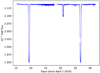 |
Fig. 1. Observed TESS light curve in units of 10−7 SAP flux vs. time (measured in days since April 1, 2020.) |
3.1.1. Light-curve modeling
In this paper, we are primarily concerned with eclipse timing and we therefore focus on those parts of the light curve showing the eclipses. Because of the somewhat unclear nature of the out-of-eclipse features of the recorded TESS light curve, we rectify the light curve by considering the pre- and post-eclipse data, fitting a third order polynomial to these data, and then dividing the measured data points by this polynomial. The result of this exercise is shown in Fig. 2 for the first primary minimum observed by TESS and in Fig. 3 for the secondary minimum. In these figures the red solid lines represent the result of our light curve modeling with nightfall3, an open source code developed by one of the authors (RW); for a more detailed description of nightfall we refer to Czesla et al. (2019a). In this paper, we use version 2.0 (released November 2022), which has been adapted for easier integration of arbitrary passbands and in particular provides support for the TESS passband. Our model of the α CrB system has effective temperatures of 10 480 K and 5755 K for the two components, and so-called Roche lobe filling factors of 0.2433 and 0.1173, respectively; the eccentricity is 0.38, the period 17.3599 days and the argument of the periapsis 312.37°. It is clear from Fig. 3 that the observed and modeled light curve shapes agree very well, hence, these rectified light curves can be used for all further timing analysis concerning the secondary minimum of α CrB.
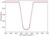 |
Fig. 2. Rectified TESS light curve of the primary minimum of α CrB on April 19, 2020; blue dots are the rectified TESS data points and the red line is a nightfall light curve model as described in the text. |
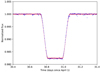 |
Fig. 3. Rectified TESS light curve of the secondary minimum of α CrB on April 30, 2020; blue dots are the rectified TESS data points and the red line is a nightfall light curve model as described in the text. |
3.1.2. Eclipse timing: Primary minimum
We first turn to the primary minima to refine Pprim, since we finally want to determine the best possible value for Pprim − Psec. The TESS light curves define the primary minima extremely well. In Fig. 4, we show the TESS data for the first observed minimum (on April 19, 2020); as evidenced by Fig. 4, we can approximate the TESS light curve around primary minimum by a parabola, which allows a straightforward calculation of the time of mid-eclipse (Tmid, ecl). To assess the errors in our determination of Tmid, ecl, we compute the residuals between observations and model fit, and then permute the so determined residuals to create new “boot-strapped” observations, for which we determine the times of mid-eclipse. Repeating this process many times, we produce a histogram of the so produced error distributions, an example of which is shown in Fig. 5. The formal dispersion is found to be 17.8 s for the minimum on April 20 and 13.5 s for May 6. These values are between 10%–15% of the bin width of the TESS data (which is 120 s), so we conclude that a reasonable and conservative error estimate of the so derived mid-eclipse times is about 25 s (or 0.00029 days) and the derived mid-eclipse times are listed in Table 2.
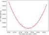 |
Fig. 4. TESS data near the primary minimum on April 19, 2020 (blue points) and best-fit parabola (red curve). |
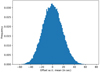 |
Fig. 5. Bootstrapped error distribution of the mid-eclipse times for the primary eclipse of α CrB on April 19, 2020 observed by TESS. |
Optical timing results for α CrB.
In this context, we want to specifically emphasize the power of the new TESS data: in contrast to all previous ground-based determinations of the minimum time of primary minimum, which required observations extending typically over many months or even years, we can now obtain our estimates from a single contiguous light curve without any folding and without any additional model assumptions. Interestingly, the time difference between the two TESS observed minima is 17.359464 days. The difference of this number from the usually adopted period is 37 s, but consistent with our error estimates of the individual primary minimum estimates; therefore, it is mandatory to include previous archival observations into the analysis to obtain a more accurate estimate of the period between primary minima.
3.1.3. Period determination: Primary minima
In Table 2, we list the available previously taken ground based measurements for primary optical eclipses; the values are taken from Tomkin & Popper (1986), who reanalyzed the photometry available from various sources dating back to 1928. In addition, we list the measurements reported by Volkov (2005).
Since we combined the measurements from different observers and observatories, a few words on the timing conventions used are in order. By default, for TESS data the time used is in the TESS Barycentric Julian Day (BTJD), that is, the Julian date minus 2457000.0 and corrected to the arrival times at the barycenter of the Solar System; these values are in the so-called Barycentric Dynamical Time frame, that is, in a time system that is not affected by leap seconds. The times used in the X-ray data analysis (both for ROSAT and XMM-Newton) are heliocentric Julian dates (HJD), which differ from the barycentric ones by a few seconds, but well below the bin size used for the X-ray data. The same system is used by Volkov (2005), yet Tomkin & Popper (1986) carried out their analysis in Julian dates without any attempt to correct to HJD or BJD values. While for individual measurements errors of up to a few minutes can be produced in this fashion, the derived mid-eclipse times result from data frequently taken over a couple of years (cf., Table 2), so that these errors should be averaged out to some extent.
We thus have measurements of primary eclipse JDP, j, j = 1...N with associated errors, σj, as well as integer values of the number of orbits elapsed Norb, j (which are known without any error) for all the times, JDP, j, and we seek a relation:

which minimizes the differences between modeled and observed times of primary minimum in a χ2 sense by adjusting the fit parameters JD0 and Pprim.
Equation (1) represents a linear regression problem, which results in the best-fit period Pprim = (17.35989517 ± 0.00000074) days and the epoch JD0 – 2444000. = (18977.24666 ± 0.00020) days. These errors were obtained by first solving Eq. (1) and then computing a Markov chain with 40000 samples; the resulting histograms are shown in Fig. 6 for the computed distributions of epochs and in Fig. 7; we note in passing that in all of our data analysis and model fitting, we made extensive use of the Python packages PyAstronomy (Czesla et al. 2019b), scipy (Virtanen et al. 2020), and the emcee package by Foreman-Mackey et al. (2013).
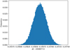 |
Fig. 6. Markov chain Monte Carlo (MCMC) posterior distribution of the epoch of the primary minimum for α CrB; numbers are given w.r.t. JD = 2458977.0 (i.e., 2020 May 7, UT 12:00). |
Interestingly, our “new” period Pprim is shorter than the previously adopted period reported by Tomkin & Popper (1986) and that difference is very much significant as demonstrated in Fig. 7, where we plot the difference (in seconds) between our best-fit period and that derived (much earlier) by Tomkin & Popper (1986). If we were to adopt, for example, the ephemerides adopted by Tomkin & Popper (1986), the minimum observed on April 19, 2020 would have had to occur 695 s later, which is clearly incompatible with the TESS observations. This difference in period is small, however, any change in Pprim compared to the period Pprim = 17.3599 d adopted by Tomkin & Popper (1986) is highly relevant for the apsidal motion values deduced.
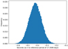 |
Fig. 7. MCMC posterior distribution of the derived period between primary minima in terms of offset in seconds w.r.t to the reference period of 17.3599 days. |
3.1.4. Eclipse timing: Secondary minimum in the optical
During secondary eclipse, the G-type star is completely occulted by the primary and the optical light curve becomes flat (cf., Fig. 3). However, as can be seen from Fig. 3, the times of first, second, third, and fourth contact are very well defined and we can define (empirically) mid-eclipse as the half time between third and second contact; we note that because of the elliptic orbit, this point in time need not coincide with the point in time when the G star, A star, and Earth are in conjunction. Specifically, we measure for the times of contacts 1–4, the values (in terms of JD – 2400000.) 58971.24058, 58971.30514, 58971.49632, and 58971.56231 respectively. This leads to the formal mid-eclipse time of 2458971.40073 listed in Table 2; it is a little difficult to assess the errors in these estimates, which we assume to be half the TESS bin width of 60 s or 0.00069 d. Furthermore, we note that the formal duration of ingress with 5578 s is shorter than that of the egress with 5701 s, which is due to the elliptic motion of the system components. Similarly, the measured eclipse and totality durations are 16 518 s and 27 798 s, respectively, which makes it clear that measurements of a single eclipse are nearly impossible from a single site on the ground.
3.2. X-ray observations
In this section, we re-utilize all the ROSAT and XMM-Newton observations of the α CrB system and, specifically, we use the ROSAT data presented and discussed by Schmitt (1998), to whom we refer for further details of the observations. We also use the XMM-Newton observations, presented, and discussed by Güdel et al. (2003). In the case of ROSAT, we use the same light curves derived by Schmitt (1998, as shown in his Fig. 1). In the case of XMM-Newton, we used the X-ray data taken with the EPIC instrument (European Photon Imaging Camera), which actually consists of two MOS detectors and one PN detector that are operated independently; for the α CrB observations the cameras were operated in the “small window” mode with the thick filter; a detailed description of the instruments can be found in the XMM-Newton Users Handbook4.
The three detectors on board XMM-Newton are operated more or less simultaneously, but not strictly simultaneously. Güdel et al. (2003) list (in their Table 1) the on-times for the individual detectors and present the X-ray light curves for their eclipse observations (in their Fig. 1). As apparent from the information provided by Güdel et al. (2003), the eclipse from January 13, 2001 is covered only very poorly during ingress and the MOS detectors produce data almost 30 min earlier than the pn-detector, which, in turn, yields data 7 min longer during egress. In the case of the eclipse on August 27, 2001, ingress is covered very well, even though the pn-detector produces data about 15 min after the MOS detectors, while during egress, the pn-detector is on more than 20 min after the MOS detectors were turned off. While Güdel et al. (2003) adjust the count rates to account for these exposure deficiencies, we decided to use the MOS data only for the January 13 eclipse (because it is essential to define the time of totality) and the pn data only for the August 27 eclipse.
The data analysis and re-processing was carried out with the XMM-Newton Science Analysis System (SAS) V 13.5 described in the Users Guide to the XMM-Newton Science Analysis System Issue 13.5, 2014 (ESA: XMM-Newton SOC). Standard SAS tools and selection criteria were used to produce X-ray event files and to generate the required data products. We specifically extracted source photons from a circular region around α CrB and the background from nearby source-free regions, however, we note that the background contributions are insignificant except for the end of the August 27 eclipse (see discussion by Güdel et al. 2003 on this point).
3.3. Combining the secondary eclipse data from ROSAT, XMM-Newton, and TESS
3.3.1. The approach
As discussed in the previous sections, we have six individual secondary eclipse measurements in the X-ray range and one eclipse measurement by TESS in the optical range, which cover an elapsed time of about 28 years. In this time span, the α CrB system executed almost 600 revolutions, thus, a difference between the period between secondary and primary minima of, say, 5 s should lead to a cumulative shift of 3000 s or 50 min, that is, far larger than the 2 min temporal resolution of the TESS data. However, the “traditional” approach, namely, determining the mid-eclipse times from the X-ray data and then proceeding with an ansatz (as in Eq. (1)) is fraught with difficulties, since the times of first to fourth contact cannot be determined that accurately; hence, the error on the derived mid-eclipse times is unclear. Also, due to the unknown inhomogeneity of α CrB B’s corona, the center of gravity of its corona might need not coincide with the center of gravity of the photospheric light.
However, if we consider a large number of X-ray eclipses, we may expect that all such coronal inhomogeneities cancel out and that such a mean X-ray eclipse shows a strong resemblance to the optical light curve of the secondary alone. Such a pure secondary light curve can be straightforwardly constructed from the data shown in Fig. 3: subtracting the flux observed during secondary eclipse, which is contributed only by the primary, from the light curve around secondary minimum. We empirically obtain the light curve contribution from the secondary alone and the shape of the mean X-ray light curve should resemble this optical secondary light curve, since we know that at X-ray wavelengths, only the secondary is contributing.
We can scale the TESS secondary light curve to some arbitrary value (we actually chose a typical X-ray count rate) and keep the time fixed in JD. All the X-ray light curves were obtained at different epochs, however, for each X-ray eclipse we know the total number of binary orbits elapsed. The knowledge of this number, together with some assumed period, allows us to shift all the observed X-ray light curves to a common time frame defined by the TESS observations and we can measure how well the shifted X-ray light curves match the so-constructed pure secondary optical light curve.
3.3.2. The implementation
In this section, we describe how the scheme described in Sect. 3.3.1 was implemented. The six X-ray light curves were obtained with different instruments, also the X-ray luminosity of α CrB may of course change from observation to observation. The X-ray fluxes of the ROSAT observations (as assessed from the out-of-eclipse data) are quite similar as evidenced by Fig. 1 in Schmitt (1998), the summed EPIC MOS rate from the transit on January 13, 2001 are quite similar to the ROSAT Position Sensitive Proportional Counter rates, only the pn-detector produced much larger rates. In this fashion, we were able to obtain X-ray rate measurements, ri, i = 1, 448 (which is the total number of ROSAT and XMM-Newton measurements used). For each value of ri we also know the times, ti, the error in ri, which is σi, and the number of orbits until the TESS observations, Norb, i. To be specific, the number of binary orbits between the TESS observations and the ROSAT observations are 585, 563, 562, and 488, respectively, and the number of binary orbits between the TESS observations and the XMM-Newton observations are 406 and 393, respectively.
As a consequence, we can associate with each point in time ti, i = 1, 448, a shifted time τi defined as:
where Psec is the sought for period between secondary minima. The thus-defined time stamps, τi, map the previously obtained X-ray data to the epoch of the TESS observed secondary minimum and we can interpolate the TESS flux on the (period-dependent) grid of τ-values. Since the coronal emission level can vary and the TESS template has an arbitrary normalization anyway, we need to additionally introduce a scaling factor, ρi, by which the observed rates, ri, are multiplied before being compared to the TESS derived secondary light curve. These scaling factors, ρi, are constant for each individual X-ray data set, thus there are only six different values of ρi in addition to the period, Psec, thereby leaving seven parameters free to vary.
In Fig. 8 (upper panel), we show the scaled and shifted X-ray light curves together with our TESS light curve template produced with nightfall. Assuming the equality of Pprim and Psec, that is, with no apsidal motion in the system, we end up with the lower panel in Fig. 8; clearly the shifted X-ray minima occur too “early,” indicating that the correct period Psec is larger than Pprim. This misbehavior is remedied by choosing an appropriate value of Psec, which yields a far better agreement between the observed TESS light curve and the shifted X-ray light curves, as shown in the upper panel of Fig. 8.
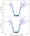 |
Fig. 8. X-ray secondary eclipse data shifted onto the scaled TESS light curve with best-fit secondary period, shown in the upper panel; blue data points refer to ROSAT data, green data points to XMM-Newton data, red curve is the best fit nightfall model to TESS; see text for details. Lower panel shows the same data as in upper panel, except that the periods between primary and secondary minima have been assumed to be identical. See text for details. |
In a frequentist scheme, we would compute the reduced  of the two models viz.
  = 3.63 for the model assuming Pprim = Psec and
  = 1.36 assuming Pprim ≠ Psec, demonstrating the high significance of our result. However, what we are really interested in is the posterior distribution of Psec. To compute this distribution, we set up a Markov chain with 280 000 elements, allowing all seven parameters to vary. The specific distribution of Psec (after burn-in) is shown in Fig. 9 as a difference with respect to the period of 17.3599 adopted by Tomkin & Popper (1986). As already clear from the
  -values, Psec is entirely incompatible with the primary period (shown in Fig. 7) and we formally find Psec = 17.3599543 ± 0.0000015 days. Therefore, the period difference is given by Psec − Pprim = 5.11 ± 0.14 s, thus conclusively proving apsidal motion in α CrB.
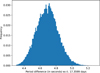 |
Fig. 9. MCMC posterior distribution of the derived period between secondary minima in terms of offset in seconds w.r.t to the reference period of 17.3599 days. |
3.4. Apsidal motion in α CrB
To deduce apsidal motion from timing measurements, we used Eq. (12), as derived in the paper by Rudkjøbing (1959), which shows that the orbit eccentricity, e, and the length of the periapsis, ω, are needed, together with their respective errors, to determine the ratio between the orbital period, P, and the period, U, of the revolution of the apsidal line. The parameters, e and ω, are best determined from radial velocity (RV) curves. Since α CrB is a double-lined spectroscopic binary, we can use the RV curves for both components obtained by Schmitt et al. (2016). For consistency with the rest of our analysis, we constructed a Markov chain, first considering the values for e and ω shown in Fig. 10. From our Markov chains, we derived e = 0.3835 ± 0.0020 and ω = 311.86 ± 0.14°, with the errors denoting the standard deviation of the posterior distribution; note that the latter value refers to the A component, that of the B component is reduced by 180°.
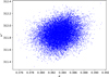 |
Fig. 10. MCMC scatter plot of eccentricity e and length of periapsis ω for the RV curves of α CrB by Schmitt et al. (2016). |
With the derived error distributions for Pprim, Psec, e, and ω, we were then able to proceed to compute P/U using Eq. (12) from Rudkjøbing (1959) by randomly sampling from these Markov chains to obtain the distribution function for P/U shown in Fig. 11; the formal values for the mean and dispersion of this distribution are 0.02441 ± 0.00070 °yr−1, implying that our analysis combining “old” optical data with modern optical data as well as including space-based X-ray measurements and optical photometry yields an apsidal motion with an accuracy of 2.9 %.
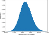 |
Fig. 11. MCMC posterior distribution for the derived apsidal motion rate |

4. Interpretation of the apsidal motion measurements in the α CrB system
4.1. Comparisons to previous works
We go on to compare our results on  obtained in this paper to the available literature estimates. As to the various values presented by Volkov (1993, 2005, 2020), it is difficult to assess the accuracy since neither the data are presented nor it is clear which assumptions went into the computation of the actual
  values. The apsidal motion rate,
  derived by Schmitt et al. (2016) by combining their new RV curve with various “historical” RV curves appears to be too large, however, already Schmitt et al. (2016) noted the inclusion of the data obtained before 1920 tends to yield larger
  values. Finally, our new apsidal motion rate is consistent with that reported by Schmitt (1998), however, given the large error of those early results this agreement might be fortuitous.
4.2. Classical apsidal motion rate
The first derivation of the classical apsidal motion rate as a result of deviations from sphericity has been given by Sterne (1939). Here, we use the formulation by Shakura (1985), who presents the apsidal motion rate from tidal and rotational effects (his Eq. (1)) and the general relativistic effect (his Eq. (2)). Using the numbers in Table 1, we can then compute a relativistic contribution of 0.0046 °yr−1 or about a fifth of the total observed apsidal motion, thus the remaining precession rate of 0.0198 °yr−1 must be caused by classical effects.
Following Shakura (1985), these classical effects can be described by an expression of the following form:
which describes the contributions of the stars (1) and (2) to the observed apsidal motion rate. The quantities k1 and k2 denote the so-called internal structure constants, which measure the degree of mass concentration of a given star. In the theory, they appear as coefficients in the expansion of the gravitational potential into Legendre polynomials, thus, the more centrally condensed a star, the smaller its internal structure coefficients become – and for a point mass, they vanish. Our internal structure constants refer only to the second order expansion and the indices refer to the stellar components, any higher order coefficients were not considered. For a precise definition and discussion of the structure coefficients, we refer to the monograph by Kopal (1978).
The coefficients ci,tid (i = 1, 2) and ci,rot (i = 1, 2) describe the effects tidal and rotational deformation caused by the two stars. To evaluate these coefficients, we need to know the masses of the two stars, their radii expressed with respect to the semi-major axis of the orbit, the rotational periods of the two stars, and the orbital period, as well as the orbit’s eccentricity and length of the periapsis; all these quantities are either known (cf., Table 1) or have been derived in this paper. We note in passing that for all our computations we used the parameters derived by Tomkin & Popper (1986), since those were derived from photometry and spectroscopy.
As can be seen from Eq. (3), the observed apsidal motion depends on the contributions from both stars and, in principle, we cannot determine two quantities (k1, k2) from one measurement (P/U). However, as we go on to show, the contributions of the primary to the total observed apsidal motion rate are by far the dominant ones; therefore, the unknown constant k1 can be determined, while no measurement of k2 can be made on the basis of our data.
Evaluating the various contributions entering Eq. (3), we first considered the rotational properties of both system components. Unfortunately, direct period measurements are not available, so we only know the measurement of vsin(i) = (139 ± 10) km s−1 from Royer et al. (2002) for the primary as well as the upper limit of about 15 km s−1 for the secondary. Let us consider first the primary and assume that its rotation axis is aligned with the orbit axis. Since the primary radius is known (cf., Table 1), we can estimate a rotation period PA of 1.07 days; if the axes were not aligned, the true equatorial rotation velocity would be even larger and the rotation period correspondingly shorter. Thus, the primary is definitely a fast rotator with a period not synchronized with the orbital period.
As to the secondary, Schmitt et al. (2016) argued that vsin(i) values of up to 5–10 km s−1 are consistent with their spectroscopic data. Furthermore, inspecting the rotational properties of the late-type Ursa Major group members studied by Ammler-von Eiff & Guenther (2009), we do not find any rapid rotators in their sample. Thus, we conclude that the secondary is certainly not a fast rotator; rather, its rotation period is likely in the range of 10–15 days, as suggested by its activity properties. It is also possible that the secondary’s rotation period might be synchronized with the orbital period and in such a case, we would expect a vsin(i) value of 2.5 km s−1.
We can trivially rewrite Eq. (3) as follows:
and we evaluate the four terms appearing on the right hand side of in Eq. (4). If the internal structure constants of the two stars were identical, we would find relative contributions of 95.01%, 4.78%, 0.13%, and 0.08% of the total effect (i.e., the expression in the outer brackets in Eq. (4)) for the coefficients c1,rot, c1,tid, c2,rot, and c2,tid, respectively. However, the internal structure constants of the two stars are not identical and according to Eq. (4), the contributions of the secondary to the total apsidal motion are weighted by the ratio  . Inspecting now the structure constants as tabulated, for example, by Hejlesen (1987) and more recently by Claret (2019), we find that the structure constants of the secondary are expected to be larger than those of the primary by factors between five and ten, namely,
  . Assuming, for example, a factor of five, these relative contributions due to the coefficients c1,rot, c1,tid, c2,rot, and c2,tid are changed to values of 94.19%, 4.74%, 0.65%, and 0.42%, respectively. These numbers therefore show that the primary by far dominates and that the contributions of the secondary amount to one percent or so of the total classic apsidal motion. Putting it differently, the rotational contribution of the primary component is expected to account for about 94% of the classical effect and the only quantity that really matters is c1,rot. As to the error in c1,rot, we note that Royer et al. (2002) quoted an error of 10 km s−1 for their value of v sin(i) or 7.1%. The error in r1 is small, Tomkin & Popper (1986) derived an error of 1.2%, and similar values are obtained for the errors in the masses of the system. We thus conclude that the error in c1,rot is dominated by the error in v1sin(i) and we therefore assume an error of 15% in c1,rot to finally obtain c1,rot = 6.40 ± 0.96 °yr−1.
4.3. Relation to internal structure constants
Combining our estimate of the “classical” precession rate of 0.0198 °yr−1 with our estimate of c1,rot, we obtained an estimate of the internal structure constant k1 for the primary of 0.0048 ± 0.00072. Theoretical determinations of internal structure coefficients have been published by various authors, so here we use the structure coefficients as a function of age as tabulated by Hejlesen (1987) and by Claret (2019). Unfortunately, these tables do not refer to stars with identical parameters. From Claret (2019), we used the structure coefficients as a function of age for a mass of 2.5 M⊙ and metalicity of Z = 0.0134, whereas from Hejlesen (1987), we used the structure coefficients for log(Mass) = 0.4 (i.e., 2.51 M⊙) and Z = 0.02 and Z = 0.04. We note that the hydrogen mass fraction X is always kept at X = 0.7. In Figs. 12 and 13, we plot both these tracks in an Hertzsprung-Russell diagram (HRD) as well as the theoretical structure coefficients derived from the underlying stellar models. In both figures, we have plotted both the individual grid points together with straight connecting lines to guide the eye; we use the same color coding and also show (in Fig. 13) our estimated value of k1 and its errors.
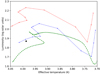 |
Fig. 12. Evolutionary tracks from the stellar structure models by Hejlesen (1987) and Claret (2019): green points and curve refer to the 2.5 M⊙ model with (X = 0.7, Z = 0.0134) from Claret (2019); blue points and curve refer to the 2.51 M⊙ model with (X = 0.7, Z = 0.02) from Hejlesen (1987); and red points and curve refer to the 2.51 M⊙ model with (X = 0.7, Z = 0.04) from Hejlesen (1987). The large black dot indicates the position of α CrB A, as computed from the parameters derived by Tomkin & Popper (1986). |
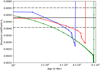 |
Fig. 13. Internal structure constant for the primary star in the α CrB system in comparison to expectations from stellar structure models by Hejlesen (1987) and Claret (2019): green points and curve refer to the 2.5 M⊙ model with (X = 0.7, Z = 0.0134) from Claret (2019); blue points and curve refer to the 2.51 M⊙ model with (X = 0.7, Z = 0.02) from Hejlesen (1987); and red points and curve refer to the 2.51 M⊙ model with (X = 0.7, Z = 0.04) from Hejlesen (1987). Black line indicates the inferred structure coefficient k1 with an error estimate of 15%. |
An inspection of the tracks of these models (plotted in Fig. 12) shows that the models from Hejlesen (1987) are far more sparsely sampled in time than those from Claret (2019); furthermore, as expected, in luminosity the different models are sorted by metalicity. The nominal position of α CrB A as computed from the parameters derived by Tomkin & Popper (1986) is also shown in Fig. 12 as the large filled circle; clearly, the high metalicity models of Hejlesen (1987) are too luminous, while the lower metalicity model of Hejlesen (1987; Z = 0.02) and the Claret (2019) model (Z = 0.0134) bracket the computed HRD position of α CrB A. Formally, the nearest grid point in the Hejlesen (1987) refers to an age of 150 Myr, that among the Claret (2019) models refers to an age of 430 Myr, yet these authors use different definitions of their adopted zero points of time. Thus, these numbers cannot be readily compared.
In Fig. 13, we show that the theoretical structure coefficients do not vary rapidly during the first few hundred Myr; also, there is no strong dependence on metalicity. All tracks considered show minima in k1 at the end of core hydrogen burning, where the luminosity and structure coefficients increase; since we estimate that the Hejlesen (1987) models must be shifted by about 100 Myr to make the time scale comparable to that used by Claret (2019), the point of core hydrogen exhaustion does not differ that much in the various models.
In summary, we conclude that all the data are consistent with α CrB A still being in its core hydrogen burning phase. The age of 414 ± 28 Myr derived by Jones et al. (2015) for the Ursa Major moving group is marginally consistent with our values, however, α CrB may in fact not be a member of this moving group. Furthermore, the ages derived by Jones et al. (2015) are quite model-dependent and the derived age dispersion of the group members depends on the inclusion of a single star. Therefore, we argue that the results by Jones et al. (2015) are not in contradiction to our structure constants. While the structure constants might indicate a somewhat younger age, the X-ray luminosity α CrB B recorded by ROSAT and XMM-Newton of 5.8 1028 erg s−1 is lower than the median X-ray luminosity for the Hyades cluster G-type stars with an age of 600 Myr (Freund et al. 2020), possibly suggesting a somewhat older age.
4.4. Spin-orbit alignment
Finally, we turn to the question of whether orbit and rotation axes in the α CrB system are aligned. Volkov (2005) suggested such a misalignment between these axes to explain the low values for the apsidal motion rate he derived. The effects of spin-orbit misalignment on apsidal motion is described by Eq. (3) in Shakura (1985) and can explain discrepancies between observed and expected apsidal motion rates. Through measurements of the Rossiter-McLaughlin effect, a spin-orbit (mis-)alignment can be directly determined and, indeed, there are well documented cases for spin orbit misalignment in, for example, CV Vel (Albrecht et al. 2013), as well as spin-orbit alignment in, for example, EP Cru (Albrecht et al. 2014). As far as α CrB A is concerned, any spin-orbit misalignment would make the derived structure constant even larger, thus, it would require a different mass distribution inside the star. Once a star has finished its contraction to the main sequence, the structure constants change rather little in the first few hundred megayears of its main sequence life; therefore, there is no need to invoke any substantial spin-orbit misalignment. In summary, all the data are consistent with assuming spin-orbit alignment and an age in the range 300–400 Myr for α CrB.
5. Conclusions
The combination of TESS, ROSAT, and XMM-Newton data allows for an unequivocal measurement of apsidal motion in α CrB. First, the TESS observations of the eclipsing α CrB system allow a refinement of the precise period between primary minima. Second, combining the TESS observation of the secondary minimum of α CrB with X-ray observations taken 20–30 years earlier allows for a similarly precise determination of the period between secondary minima. The difference between these two periods is found to be 5.15 ± 0.14 s, which in turn allows to compute the apsidal motion in this system, using suitable values of eccentricity and the length of the periapsis.
These new data conclusively end the long debate on the significance of the available apsidal motion measurements in this system. The apsidal motion precession period of the system is found to be 18 200 yr with an error of about 2.9%; the general relativistic contribution to the apsidal motion amounts to 15% of the overall effect. We demonstrate that the deformation of the A component due to its very rapid rotation is almost solely responsible for the remaining “classical” apsidal motion effect. The resulting internal stellar structure coefficient agrees well with model computations for a young (age about 300 Myr) main sequence star with solar metalicity and an aligned spin-orbit geometry. The spin-orbit alignment could be tested with Rossiter-McLaughlin measurements and further TESS observations of primary and, in particular, secondary eclipses would allow us to refine the period measurements even further.
Note that the denominator in the second term of Eq. (3) of Schmitt (1998) must read (1 − e2)5.
Acknowledgments
We specifically thank the efforts of the XMM-Newton User support who made the data set on α CrB from January 2001 available to us. Furthermore, SC acknowledges support from DFG through grant CZ 222/5-1. This paper includes data collected with the TESS mission, obtained from the MAST data archive at the Space Telescope Science Institute (STScI). Funding for the TESS mission is provided by the NASA Explorer Program. STScI is operated by the Association of Universities for Research in Astronomy, Inc., under NASA contract NAS 5-26555.
References
- Albrecht, S., Setiawan, J., Torres, G., et al. 2013, ApJ, 767, 32 [NASA ADS] [CrossRef] [Google Scholar]
- Albrecht, S., Winn, J. N., Torres, G., et al. 2014, ApJ, 785, 83 [CrossRef] [Google Scholar]
- Ammler-von Eiff, M., & Guenther, E. W. 2009, A&A, 508, 677 [NASA ADS] [CrossRef] [EDP Sciences] [Google Scholar]
- Claret, A. 2019, A&A, 628, A29 [NASA ADS] [CrossRef] [EDP Sciences] [Google Scholar]
- Claret, A., Giménez, A., Baroch, D., et al. 2021, A&A, 654, A17 [NASA ADS] [CrossRef] [EDP Sciences] [Google Scholar]
- Czesla, S., Terzenbach, S., Wichmann, R., et al. 2019a, A&A, 623, A107 [NASA ADS] [CrossRef] [EDP Sciences] [Google Scholar]
- Czesla, S., Schröter, S., Schneider, C. P., et al. 2019b, Astrophysics Source Code Library, [record ascl:1906.010] [Google Scholar]
- Ebbighausen, E. G. 1976, Pub. Dominion Astrophys. Obs. Victoria, 14, 411 [Google Scholar]
- Foreman-Mackey, D., Hogg, D. W., Lang, D., et al. 2013, PASP, 125, 306 [NASA ADS] [CrossRef] [Google Scholar]
- Freund, S., Robrade, J., Schneider, P. C., et al. 2020, A&A, 640, A66 [NASA ADS] [CrossRef] [EDP Sciences] [Google Scholar]
- Güdel, M., Arzner, K., Audard, M., & Mewe, R. 2003, A&A, 403, 155 [NASA ADS] [CrossRef] [EDP Sciences] [Google Scholar]
- Hejlesen, P. M. 1987, A&AS, 69, 251 [NASA ADS] [Google Scholar]
- Jenkins, J. M., Twicken, J. D., McCauliff, S., et al. 2016, Proc. SPIE, 9913, 99133E [Google Scholar]
- Jones, J., White, R. J., Boyajian, T., et al. 2015, ApJ, 813, 58 [NASA ADS] [CrossRef] [Google Scholar]
- Koch, R. H. 1973, ApJ, 183, 275 [NASA ADS] [CrossRef] [Google Scholar]
- Kopal, Z. 1978, Astrophys. Space Sci. Lib., 68 [Google Scholar]
- Kron, G. E., & Gordon, K. C. 1953, ApJ, 118, 55 [NASA ADS] [CrossRef] [Google Scholar]
- Nouh, M. I., Saad, S. M., Korany, B., et al. 2013, J. Astrophys. Astron., 34, 193 [NASA ADS] [CrossRef] [Google Scholar]
- Ricker, G. R., Winn, J. N., Vanderspek, R., et al. 2015, J. Astron. Telesc. Instrum. Syst., 1, 014003 [Google Scholar]
- Royer, F., Grenier, S., Baylac, M.-O., Gómez, A. E., & Zorec, J. 2002, A&A, 393, 897 [NASA ADS] [CrossRef] [EDP Sciences] [Google Scholar]
- Rudkjøbing, M. 1959, Annales d’Astrophysique, 22, 111 [NASA ADS] [Google Scholar]
- Russell, H. N. 1947, Harvard College Obs. Circ., 451 [Google Scholar]
- Russell, H. N. 1948, Harvard Obs. Monogr., 181 [Google Scholar]
- Schmitt, J. H. M. M. 1998, A&A, 333, 199 [NASA ADS] [Google Scholar]
- Schmitt, J. H. M. M., & Kürster, M. 1993, Science, 262, 215 [NASA ADS] [CrossRef] [Google Scholar]
- Schmitt, J. H. M. M., Schröder, K.-P., Rauw, G., et al. 2014, Astron. Nachr., 335, 787 [NASA ADS] [CrossRef] [Google Scholar]
- Schmitt, J. H. M. M., Schröder, K.-P., Rauw, G., et al. 2016, A&A, 586, A104 [NASA ADS] [CrossRef] [EDP Sciences] [Google Scholar]
- Shakura, N. I. 1985, Soviet Astron. Lett., 11, 224 [Google Scholar]
- Southworth, J. 2012, Orbital Couples: Pas de Deux in the Solar System and the Milky Way, 51 [Google Scholar]
- Stebbins, J. 1928, Pub. Washburn Obs., 15, 41 [Google Scholar]
- Sterne, T. E. 1939, MNRAS, 99, 451 [NASA ADS] [Google Scholar]
- Tomkin, J., & Popper, D. M. 1986, AJ, 91, 1428 [NASA ADS] [CrossRef] [Google Scholar]
- Virtanen, P., Gommers, R., Oliphant, T. E., et al. 2020, Nat. Methods, 17, 261 [Google Scholar]
- Volkov, I. M. 1993, Inf. Bull. Var. Stars, 3876, 1 [NASA ADS] [Google Scholar]
- Volkov, I. M. 2005, Ap&SS, 296, 105 [NASA ADS] [CrossRef] [Google Scholar]
- Volkov, I. M. 2020, Contrib. Astron. Obs. Skalnate Pleso, 50, 635 [NASA ADS] [Google Scholar]
All Tables
All Figures
|
Fig. 1. Observed TESS light curve in units of 10−7 SAP flux vs. time (measured in days since April 1, 2020.) |
| In the text | |
|
Fig. 2. Rectified TESS light curve of the primary minimum of α CrB on April 19, 2020; blue dots are the rectified TESS data points and the red line is a nightfall light curve model as described in the text. |
| In the text | |
|
Fig. 3. Rectified TESS light curve of the secondary minimum of α CrB on April 30, 2020; blue dots are the rectified TESS data points and the red line is a nightfall light curve model as described in the text. |
| In the text | |
|
Fig. 4. TESS data near the primary minimum on April 19, 2020 (blue points) and best-fit parabola (red curve). |
| In the text | |
|
Fig. 5. Bootstrapped error distribution of the mid-eclipse times for the primary eclipse of α CrB on April 19, 2020 observed by TESS. |
| In the text | |
|
Fig. 6. Markov chain Monte Carlo (MCMC) posterior distribution of the epoch of the primary minimum for α CrB; numbers are given w.r.t. JD = 2458977.0 (i.e., 2020 May 7, UT 12:00). |
| In the text | |
|
Fig. 7. MCMC posterior distribution of the derived period between primary minima in terms of offset in seconds w.r.t to the reference period of 17.3599 days. |
| In the text | |
|
Fig. 8. X-ray secondary eclipse data shifted onto the scaled TESS light curve with best-fit secondary period, shown in the upper panel; blue data points refer to ROSAT data, green data points to XMM-Newton data, red curve is the best fit nightfall model to TESS; see text for details. Lower panel shows the same data as in upper panel, except that the periods between primary and secondary minima have been assumed to be identical. See text for details. |
| In the text | |
|
Fig. 9. MCMC posterior distribution of the derived period between secondary minima in terms of offset in seconds w.r.t to the reference period of 17.3599 days. |
| In the text | |
|
Fig. 10. MCMC scatter plot of eccentricity e and length of periapsis ω for the RV curves of α CrB by Schmitt et al. (2016). |
| In the text | |
|
Fig. 11. MCMC posterior distribution for the derived apsidal motion rate |
| In the text | |
|
Fig. 12. Evolutionary tracks from the stellar structure models by Hejlesen (1987) and Claret (2019): green points and curve refer to the 2.5 M⊙ model with (X = 0.7, Z = 0.0134) from Claret (2019); blue points and curve refer to the 2.51 M⊙ model with (X = 0.7, Z = 0.02) from Hejlesen (1987); and red points and curve refer to the 2.51 M⊙ model with (X = 0.7, Z = 0.04) from Hejlesen (1987). The large black dot indicates the position of α CrB A, as computed from the parameters derived by Tomkin & Popper (1986). |
| In the text | |
|
Fig. 13. Internal structure constant for the primary star in the α CrB system in comparison to expectations from stellar structure models by Hejlesen (1987) and Claret (2019): green points and curve refer to the 2.5 M⊙ model with (X = 0.7, Z = 0.0134) from Claret (2019); blue points and curve refer to the 2.51 M⊙ model with (X = 0.7, Z = 0.02) from Hejlesen (1987); and red points and curve refer to the 2.51 M⊙ model with (X = 0.7, Z = 0.04) from Hejlesen (1987). Black line indicates the inferred structure coefficient k1 with an error estimate of 15%. |
| In the text | |
Current usage metrics show cumulative count of Article Views (full-text article views including HTML views, PDF and ePub downloads, according to the available data) and Abstracts Views on Vision4Press platform.
Data correspond to usage on the plateform after 2015. The current usage metrics is available 48-96 hours after online publication and is updated daily on week days.
Initial download of the metrics may take a while.