© The Authors 2023

1. Introduction

Rotation is ubiquitous in both stars and planets, and it has a profound effect on their structure and evolution. For instance, recent interferometric observations have shown to what extent stars can be affected by centrifugal deformation and gravity darkening (e.g., Domiciano de Souza et al. 2003; Monnier et al. 2007; Zhao et al. 2009; Che et al. 2011; Bouchaud et al. 2020). Various studies have predicted (Endal & Sofia 1976; Zahn 1992; Maeder & Zahn 1998; Mathis & Zahn 2004) and shown (Meynet & Maeder 2000; Palacios et al. 2003, 2006; Amard et al. 2019) its impact on stellar evolution and raised a number of open questions (e.g., Deheuvels et al. 2012, 2015; Benomar et al. 2015; Ouazzani et al. 2019. The monograph by Maeder (2009) provides a comprehensive description of the impact of rotation on stellar evolution from a theoretical standpoint, while Aerts et al. (2019) provided a recent review that focused on transport processes in these stars and the resulting open questions. Likewise, rotation plays an important role in gas giants such as Jupiter and Saturn. It proved critical to take centrifugal deformation into account when interpreting the gravitational moments of Jupiter measured by Juno in order to investigate the presence of a core (e.g., Wahl et al. 2017) or to probe the wind gradient and differential rotation (e.g., Iess et al. 2018; Guillot et al. 2018). Furthermore, the recent detection of f-modes¹ (e.g., Hedman & Nicholson 2013) and g-modes (Mankovich & Fuller 2021) in Saturn has sparked kronoseismic² investigations into Saturn’s core, which required taking the effects of rotation on Saturn’s structure and pulsations into account (Fuller 2014; Mankovich et al. 2019; Dewberry et al. 2021). Hence, there is a real need for numerical tools that are able to calculate the structure of these stars and planets.

In the stellar domain, much progress has been made over the past years in devising 2D stellar structure codes that fully take rotation into account. For instance, the Self-Consistent Field (SCF) method has been devised to calculate the structure of stars with pre-imposed cylindrical rotation profiles (Jackson et al. 2005; MacGregor et al. 2007). It alternates between solving Poisson’s equation and the hydrostatic equilibrium, thereby iteratively adjusting the distribution of matter in the star. Because the rotation profile is conservative, the structure of the star is barotropic, which means that lines of constant pressure, density, temperature, and thus the total (gravitational and centrifugal) potential coincide. Hence, solving the hydrostatic equilibrium amounts to finding the lines of constant total potential and redistributing the matter so that the density is constant along these lines.

A drawback of the SCF method is that the energy equation is only solved along horizontal averages rather than locally. To overcome this difficulty, the Evolution STEllaire en Rotation code (ESTER) was developed (Espinosa Lara & Rieutord 2013; Rieutord et al. 2016). As a result of solving the energy equation locally, the rotation profile (which is calculated along with the stellar structure) is no longer conservative, and the stellar structure is baroclinic, that is, isodensity and isobars are now free to differ. Currently, neither code is capable of carrying out stellar evolution, and the codes instead calculate static models. The composition within ESTER models may nonetheless be adjusted to mimic the effects of stellar evolution.

A solution for bypassing the above limitation is to take stellar models from 1D non-rotating stellar evolution codes and to subsequently introduce the effects of centrifugal deformation. This is the strategy introduced in Roxburgh (2006). The author used the density profile from the 1D model, applied it along a radial cut (at some given latitude), and then iteratively reconstructed the distribution of matter in the rest of the star for a predefined 2D rotation profile. From there, the pressure distribution and gravitational field may be calculated. In addition, if an assumption is made on the chemical composition, then it is possible to deduce the adiabatic exponent, Γ₁, throughout the star through the equation of state, followed by variables such as the sound velocity and the Brunt-Väisälä frequency. Hence, a complete acoustic structure is obtained that allows the calculation of pulsation modes (Ouazzani et al. 2015).

One of the limitations of this method is that the energy equation is not taken to account and is thus not generally satisfied. To overcome this difficulty, this method may be applied to 1D models where the effects of rotation are already taken into account, albeit in an approximate way. For instance, models from the Grenoble stellar evolution code (STAREVOL; Palacios et al. 2003, 2006), the Geneva stellar evolution code (Eggenberger et al. 2008), and the Code d’Evolution Stellaire Adaptatif et Modulaire with Transport (CESTAM; Marques et al. 2013) take into account the horizontally averaged effects of rotation through the formalism developed in Zahn (1992) and Maeder & Zahn (1998). Manchon (2021) developed a method that is more elaborate because it calculates the centrifugal deformation for CESTAM models, but then feeds the information from the 2D structure back into the 1D formalism using the approach described in Mathis & Zahn (2004). Such a procedure could then be applied at each time step when the evolution of a star is calculated, and a greater degree of realism can be achieved in this way.

In this article, we wish to develop a method analogous to that of Roxburgh (2006) but that is simpler. In particular, we wish to avoid having to reuse the equation of state to recalculate the Γ₁ profile. The resulting program, the Rotation code Using Barotropy conservation over Isopotential Surfaces (https://github.com/pierrehoudayer/RUBIS), achieves this by preserving the relation between density and pressure rather than density and radius when going from the 1D to the 2D structure, as we describe below. Hence, the equation of state is automatically satisfied throughout the model because thermodynamic quantities are simply carried over from the 1D case. With this approach, deforming a 1D polytropic structure, for instance, leads to a 2D polytropic structure, unlike what would happen with the approach in Roxburgh (2006). Finally, we wish to make this approach applicable to stars and planets, which may include density discontinuities. Models with discontinuities require applying a different strategy when solving Poisson’s equation, as we explain below.

As was the case with the approach developed in Roxburgh (2006), RUBIS does not take the energy conservation equation into account. Hence, the models it deforms will only be suitable for adiabatic pulsation calculations. For full non-adiabatic calculations, models such as those from the ESTER code should be used instead, in which the hydrostatic structure and the energy equation are solved in a full 2D context.

The article is organised as follows: Sect. 2 begins by explaining how our code, RUBIS, works, and Sect. 3 emphasises the specific features that differentiate it from existing programs. Section 4 is devoted to carrying out numerical tests, in particular, comparisons with existing programs, and it establishes the scope within which the assumptions we adopted are valid. Section 5 is dedicated to our conclusion and more broadly, to our perspectives on the future use of RUBIS.

2. Description of RUBIS

As stated in the introduction, the starting point of the method is to assume that the relation between ρ and P is preserved when going from the non-rotating to the rotating models. This can be justified in one of two ways: either some intrinsic relation exists between ρ and P, for instance, the polytropic relation, or we assume that the thermodynamic structure of the non-rotating model is in some sense a good approximation of the structure of the rotating model. We discuss this assumption in Sects. 3 and 4. We now derive the direct implication of this assumption, which is also the key property of RUBIS.

The hydrostatic equilibrium of a rotating, self-gravitating object (with a conservative rotation profile) is described by the following equation:

$$\begin{array}{c}\hfill \mathbf{\nabla }P=-\rho \mathbf{\nabla }{\mathrm{\Phi }}_{\mathrm{eff}},\end{array}$$(1)

where P is the pressure, ρ is the density, and Φ_eff = Φ_G + Φ_C is the total potential, Φ_G being the gravitational potential and Φ_C the centrifugal potential. These potentials satisfy the following equations:

$$\begin{array}{cc}\hfill \mathrm{\Delta }{\mathrm{\Phi }}_{\mathrm{G}}& =4\pi \mathcal{G}\rho ,\hfill \end{array}$$(2)

$$\begin{array}{cc}\hfill {\mathrm{\Phi }}_{\mathrm{C}}& =-{\displaystyle {\int }_0^s}{\mathrm{\Omega }}^2(s^{\prime })s^{\prime }\mathrm{d}{s}^{\prime },\hfill \end{array}$$(3)

where 𝒢 is the gravitational constant, Ω(s) is the rotation profile, and s is the distance to the rotation axis. We recall that conservative rotation profiles are cylindrical, that is, they only depend on the distance to the rotation axis. This property allows the centrifugal force to derive from a potential and leads to a barotropic structure for the object, as can be seen by taking the curl of Eq. (1) divided by the density: ∇ρ × ∇P = 0.

We introduce a coordinate system (ζ, θ, φ) such that ζ is constant along isopotential lines, and where θ and φ denote the usual polar and azimuthal angles. At this stage, ζ is a dimensionless variable used to label the isopotential lines and is not a physical coordinate. This means that there are no requirements on what values it takes as long as it varies smoothly and monotonically from the centre of the star or planet to the surface. Accordingly, given the barotropic structure of the deformed object, quantities such as P and ρ only depend on ζ. Hence, projected on the natural basis, we can show that Eq. (1) reduces to

$$\begin{array}{c}\hfill \frac{\mathrm{d}P}{\mathrm{d}\zeta }=-\rho \frac{\mathrm{d}{\mathrm{\Phi }}_{\mathrm{eff}}}{\mathrm{d}\zeta },\end{array}$$(4)

the other components being zero. This equation can be compared with its non-rotating equivalent,

$$\begin{array}{c}\hfill \frac{\mathrm{d}{P}_{\mathrm{sph}}}{\mathrm{d}{r}_{\mathrm{sph}}}=-{\rho }_{\mathrm{sph}}\frac{\mathrm{d}{\mathrm{\Phi }}_{\mathrm{sph}}}{\mathrm{d}{r}_{\mathrm{sph}}},\end{array}$$(5)

where Φ_sph reduces to the gravitational potential, and where the notation r_sph has been introduced to avoid confusion between r in the rotating and non-rotating models. It is possible to choose the values of ζ in such a way that P(ζ)≡P_sph(r_sph) given that P is a monotonic function of ζ. As a result, dP/dζ = dP_sph/dr_sph immediately follows. Furthermore, preserving the relation between ρ and P when going from the non-rotating and to the rotating model also leads to ρ(ζ) = ρ_sph(r_sph), and this holds regardless of whether ρ varies monotonically with ζ. The hydrostatic equations then show that dΦ_eff/dζ = dΦ_sph/dr_sph. In other words,

$$\begin{array}{c}\hfill {\mathrm{\Phi }}_{\mathrm{eff}}(\zeta )={\mathrm{\Phi }}_{\mathrm{sph}}(r_{\mathrm{sph}})+\mathrm{cnst}.\end{array}$$(6)

The constant that appears in this equation may in fact be deduced by applying the above equation at the object’s centre, that is, r_sph = ζ = 0 (assuming the gravitational components of both potentials match a vacuum potential outside the deformed object).

These observations lead us to outline the following iterative approach, which is a simplified version of the SCF algorithm (Jackson et al. 2005; MacGregor et al. 2007):

1. Find the gravitational potential based on the matter distribution (Sect. 2.1).

2. Add the centrifugal potential to the gravitational potential (Sect. 2.2).

3. Find the level surfaces, that is, the lines of constant total potential, and redistribute the matter on these surfaces (Sect. 2.3).

4. Return to step 1 and iterate until convergence (Sect. 2.4).

Figure 1 illustrates this algorithm schematically. These steps are described in more detail below.

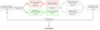Fig. 1. Flowchart illustrating how RUBIS works. Each step shows the quantity that is obtained and in terms of which variable it is obtained.

2.1. Finding the gravitational potential

There are two different ways of calculating the gravitational potential. The first approach consists in interpolating the matter distribution onto the spherical coordinate system and solving Poisson’s equation after having projected it onto the spherical harmonic basis (Sect. 2.1.1). The second approach consists in solving Poisson’s equation using the spheroidal coordinate system directly (Sect. 2.1.2).

2.1.1. Using spherical coordinates

Although the first approach may sound more complicated because of the additional interpolation step, it is in fact more efficient. When the matter distribution is expressed using spherical coordinates, Poisson’s equation becomes separable with respect to the spherical harmonic basis. This allows it to be solved efficiently.

The interpolation of the density profile onto the spherical coordinate system is carried out using cubic splines along each latitude with the SciPy sub-package scipy.interpolate³. Afterwards, the density profile is decomposed using the spherical harmonic basis as follows:

$$\begin{array}{c}\hfill \rho (r,\theta ,\phi )={\displaystyle \sum _{\ell =0}^{\infty }\sum _{m=-\ell }^{\ell }{\rho }_{\ell }^m(r)Y_{\ell }^m(\theta ,\phi ),}\end{array}$$(7)

where

$$\begin{array}{c}\hfill {\rho }_{\ell }^m(r)={\displaystyle \int {\int }_{4\pi }\rho (r,\theta ,\phi ){\left[Y_{\ell }^m(\theta ,\phi )\right]}^{\ast }sin\theta \mathrm{d}\theta \mathrm{d}\phi ,}\end{array}$$(8)

and where ℓ represents the harmonic degree, m the azimuthal order, $Y_{\mathcal{l}}^m$ the corresponding spherical harmonic, and ( ⋅ )^* the complex conjugate. Because the deformed object is axisymmetric, only the m = 0 components of ρ and Φ_G are non-zero. Hence, in what follows, we assume m = 0 and drop the m index. On a practical level, the manipulation of harmonic series, whether for decomposition or projection, is implemented in RUBIS using the appropriate scipy.special⁴ routines.

Poisson’s equation is subsequently projected onto the spherical harmonic basis, thus leading to

$$\begin{array}{c}\hfill \frac{{\mathrm{d}}^2{\mathrm{\Phi }}_{\mathrm{G}}^{\ell }}{\mathrm{d}{r}^2}+\frac{2}{r}\frac{\mathrm{d}{\mathrm{\Phi }}_{\mathrm{G}}^{\ell }}{\mathrm{d}r}-\frac{\ell (\ell +1)}{r^2}{\mathrm{\Phi }}_{\mathrm{G}}^{\ell }=4\pi \mathcal{G}{\rho }_{\ell }\end{array}$$(9)

for each spherical harmonic. Here, ${\mathrm{\Phi }}_{\text{G}}^{\mathcal{l}}$ represents the projection of Φ_G onto the harmonic basis. Equation (9) can be solved analytically using integrals,

$$\begin{array}{c}\hfill {\mathrm{\Phi }}_{\mathrm{G}}^{\ell }=-\frac{4\pi \mathcal{G}}{2\ell +1}{\displaystyle [{\int }_0^r{\rho }_{\ell }(s)\frac{s^{\ell +2}}{r^{\ell +1}}\mathrm{d}s+{\int }_r^R{\rho }_{\ell }(s)\frac{r^{\ell }}{s^{\ell -1}}\mathrm{d}s],}\end{array}$$(10)

where R is the stellar radius. However, when ℓ becomes large, the above formula can lead to poor numerical results. Therefore, we prefer to solve Eq. (9) numerically by first casting it into a first-order system of two differential equations, discretising it using the finite-difference approach described in Reese (2013), and solving the system with an efficient band matrix factorisation using the appropriate Lapack⁵ wrapper available in scipy.linalg.lapack⁶. This requires including boundary conditions that ensure the continuity of ${\mathrm{\Phi }}_{\text{G}}^{\mathcal{l}}$ and its derivative on the object’s surface,

$$\begin{array}{cc}\hfill {\mathrm{\Phi }}_G^{\ell ,\mathrm{in}}(R)& ={\mathrm{\Phi }}_G^{\ell ,\mathrm{out}}(R)\hfill \end{array}$$(11)

$$\begin{array}{cc}\hfill {\frac{\mathrm{d}{\mathrm{\Phi }}_G^{\ell ,\mathrm{in}}}{\mathrm{d}r}|}_R& ={\frac{d{\mathrm{\Phi }}_G^{\ell ,\mathrm{out}}}{\mathrm{d}r}|}_R.\hfill \end{array}$$(12)

In addition, we also apply regularity conditions in the centre and at infinity,

$$\begin{array}{cc}& {\mathrm{\Phi }}_G^{\ell }(r)\underset{r\to 0}{\propto }{r}^{\ell }\hfill \end{array}$$(13)

$$\begin{array}{cc}& {\mathrm{\Phi }}_G^{\ell }(r)\underset{r\to \infty }{\propto }{r}^{-(\ell +1)}.\hfill \end{array}$$(14)

Combining the latter equation with Eqs. (11) and (12) then leads to the following condition on the object’s surface (e.g., Ledoux & Walraven 1958):

$$\begin{array}{c}\hfill \frac{\mathrm{d}{\mathrm{\Phi }}_{\mathrm{G}}^{\ell }}{\mathrm{d}r}(R)+\frac{\ell +1}{R}{\mathrm{\Phi }}_{\mathrm{G}}^{\ell }(R)=0.\end{array}$$(15)

Equations (9) together with conditions (13) and (15) are solved up to a certain degree, L, which is fixed by the user at the beginning of the procedure. When the ${\mathrm{\Phi }}_{\text{G}}^{\mathcal{l}}$(r) functions have been obtained, the potential is then deduced in terms of the (r, θ) coordinates using

$$\begin{array}{c}\hfill {\mathrm{\Phi }}_{\mathrm{G}}(r,\theta )={\displaystyle \sum _{\ell =0}^{\infty }{\mathrm{\Phi }}_{\mathrm{G}}^{\ell }(r)Y_{\ell }^0(\theta ).}\end{array}$$(16)

2.1.2. Using spheroidal coordinates

This approach does not function correctly when the density profile is discontinuous. A discontinuity in the density profile will follow a level surface due to the barotropic structure of the object. Hence, it will intersect spherical surfaces thus causing the density profile to be discontinuous as a function of latitude for certain values of r. This leads to poor numerical results when the density profile is projected onto the spherical harmonic basis and may stop the algorithm from converging.

Accordingly, Poisson’s equation must be solved directly in the spheroidal coordinate system, (ζ, θ, φ). Hence, the following harmonic decomposition is used instead:

$$\begin{array}{c}\hfill {\mathrm{\Phi }}_{\mathrm{G}}(\zeta ,\theta )={\displaystyle \sum _{\ell =0}^{\infty }{\mathrm{\Phi }}_{\mathrm{G}}^{\ell }(\zeta )Y_{\ell }^0(\theta ).}\end{array}$$(17)

When we treat the radial distance, r, as a function of ζ and θ, we obtain through tensor analysis (cf. Appendix A) the following explicit expression for Poisson’s equation:

$$\begin{array}{c}\hfill {\partial }_{\zeta }\left(\frac{r^2+r_{\theta }^2}{r_{\zeta }}{\partial }_{\zeta }{\mathrm{\Phi }}_{\mathrm{G}}\right)-2r_{\theta }{\partial }_{\zeta \theta }^2{\mathrm{\Phi }}_{\mathrm{G}}-{\mathrm{\Delta }}_{\mathcal{S}}r{\partial }_{\zeta }{\mathrm{\Phi }}_{\mathrm{G}}+r_{\zeta }{\mathrm{\Delta }}_{\mathcal{S}}{\mathrm{\Phi }}_{\mathrm{G}}=4\pi \mathcal{G}{r}^2{r}_{\zeta }\rho ,\end{array}$$(18)

where

$$\begin{array}{c}\hfill {\mathrm{\Delta }}_{\mathcal{S}}={\partial }_{\theta \theta }^2+cot\theta {\partial }_{\theta },\end{array}$$(19)

and where r_ζ = ∂_ζr, r_θ = ∂_θr, $r_{\zeta \theta }={\partial }_{\zeta \theta }^{2}r$, and so on. We note that due to the symmetry around the rotation axis, derivatives with respect to φ vanish.

This equation is then projected onto the spherical harmonic basis, discretised in the radial direction using finite differences, and solved. Because of its expression, Eq. (18) is not separable on the spherical harmonic basis. Hence, the equations for the different ${\mathrm{\Phi }}_{\text{G}}^{\mathcal{l}}$ are coupled,

$$\begin{array}{c}\hfill {\displaystyle \sum _{{\ell }^{\prime }=0}^L}{\partial }_{\zeta }\left({\mathcal{P}}_{\zeta \zeta }^{\ell {\ell }^{\prime }}{\partial }_{\zeta }{\mathrm{\Phi }}_{\mathrm{G}}^{{\ell }^{\prime }}\right)-{\mathcal{P}}_{\zeta \theta }^{\ell {\ell }^{\prime }}{\partial }_{\zeta }{\mathrm{\Phi }}_{\mathrm{G}}^{{\ell }^{\prime }}-{\mathcal{P}}_{\theta \theta }^{\ell {\ell }^{\prime }}{\mathrm{\Phi }}_{\mathrm{G}}^{{\ell }^{\prime }}=4\pi \mathcal{G}{(r^2{r}_{\zeta })}_{\ell }\rho ,\end{array}$$(20)

which results in the appearance of coupling integrals, ${\mathcal{P}}_{··}^{\ell \ell \prime }$, as well as the harmonic decomposition of r²r_ζ denoted (r²r_ζ)_ℓ (we refer to Appendix A for an explicit expression of the terms appearing in Eq. (20)). These equations must then be solved simultaneously. However, the use of finite differences means that only adjacent values of ζ are coupled. Hence, grouping together the unknowns, ${\mathrm{\Phi }}_{\text{G}}^{\mathcal{l}}$(ζ_i), according to ζ values leads to a band matrix (although of much larger dimensions than when solving Eq. (9)), which can be filled efficiently using the scipy.sparse⁷ package, and which is once more solved with the Lapack routine.

In order to ensure that the potential matches a vacuum potential outside the deformed object, a second domain is added with the object’s surface as an inner boundary and a sphere as the outer boundary. Poisson’s equation is then enforced on this domain subject to interface conditions on the inner boundary in order to ensure the continuity of the gravitational potential and its gradient which, in terms of the spheroidal coordinates, results in preserving $r_{\zeta }{}^{-1}{\partial }_{\zeta }{\mathrm{\Phi }}_{\text{G}}$ in addition to Φ_G through the surface. In the case of internal density discontinuities, these two conditions (derived in Eqs. (A.11) and (A.18)) must be added at each of the domain interfaces. Finally, conditions analogous to Eqs. (13) and (15) are applied in the centre and on the outer spherical boundary.

Once more, Φ_G(ζ, θ) can subsequently be deduced from the ${\mathrm{\Phi }}_{\text{G}}^{\mathcal{l}}$(ζ) using Eq. (17). It should be noted that the latter equation implicitly also gives us the gravitational potential as a function of r and θ by using the relation r(ζ, θ) since Φ_G(r(ζ, θ),θ)  =  Φ_G(ζ, θ).

2.2. Adding the centrifugal potential

Whether solving Poisson’s equation in spherical (cf. Sect. 2.1.1) or spheroidal (cf. Sect. 2.1.2) coordinates, we derived the gravitational potential Φ_G(r, θ) at this point. The total potential at any point in the structure is therefore determined by simply adding the centrifugal potential Φ_C(r, θ). As mentioned above, the latter must satisfy a cylindrical symmetry in order to preserve the barotropic relation. As a consequence, this approach cannot be used on potentials derived from shellular rotation profiles, that is, Ω = Ω(r), for instance. However, we note the large number of profiles that can be used because any 1D rotation profile integrated using Eq. (3) could lead to an eligible Φ_C(s) in theory. In practice, it may be advisable to check that at least the Rayleigh criterion for stability is verified: ∂_r(r⁴Ω²) > 0.

After it is chosen, the integration of the rotation profile may lead to analytical expressions for the centrifugal potential. Typical examples are those involving solid rotation,

$$\begin{array}{c}\hfill \mathrm{\Omega }(s)={\mathrm{\Omega }}_0\to {\mathrm{\Phi }}_{\mathrm{C}}(r,\theta )=-\frac{1}{2}{s}^2{\mathrm{\Omega }}_0^2,\end{array}$$(21)

or a Lorentzian profile,

$$\begin{array}{c}\hfill \mathrm{\Omega }(s)=\frac{1+\alpha }{1+\alpha {(s/R_{\mathrm{eq}})}^2}{\mathrm{\Omega }}_0\to {\mathrm{\Phi }}_{\mathrm{C}}(r,\theta )=-\frac{1}{2}\frac{{(1+\alpha )}^2{s}^2{\mathrm{\Omega }}_0^2}{1+\alpha {(s/R_{\mathrm{eq}})}^2},\end{array}$$(22)

where s = r sin θ and Ω₀ and α designate the rotation rate on the equator and the relative difference on the rotation rate between the centre and equator, respectively.

2.3. Finding level surfaces and redistributing matter

When the total potential Φ_eff(r, θ) has been calculated, level surfaces may be obtained by finding isopotential lines. As a first step, Eq. (6) shows that the total potential just found must satisfy

$$\begin{array}{c}\hfill {\mathrm{\Phi }}_{\mathrm{eff}}(r,\theta )={\mathrm{\Phi }}_{\mathrm{sph}}(r_{\mathrm{sph}})+\mathrm{cnst},\end{array}$$(23)

meaning that the latter can be deduced from the initial (spherical) potential to which a suitable constant has been added. The value of this constant is immediately found by applying the same relation at the model’s centre,

$$\begin{array}{c}\hfill \mathrm{cnst}={\mathrm{\Phi }}_{\mathrm{G}}(0,0)+{\mathrm{\Phi }}_{\mathrm{C}}(0,0)-{\mathrm{\Phi }}_{\mathrm{sph}}(0).\end{array}$$(24)

Therefore, a given level surface r_*(θ) (corresponding to a certain ζ_*) can be deduced from the freshly calculated potential Φ_eff(r, θ) by satisfying Eq. (23) for all θ, using the constant provided by Eq. (24). As explained at the start of the section, choosing level surfaces in this way ensures that the correspondence between ρ(ζ) and ρ_sph(r_sph) is preserved for ζ = r_sph.

The level surfaces can be found in many different ways. In our algorithm, we decompose f(r) = Φ_eff(r, θ) as a sum of Hermite splines because both Φ_eff and ∂_rΦ_eff are available. Using the current level surfaces as a first guess, we can now use Newton’s method to find the new r values satisfying Eq. (23). This approach can reach a high degree of accuracy fairly quickly given the efficiency of Newton’s method and because the positions of level surfaces change progressively less during the successive iterations, thus causing the first guess to become very close to the actual solution.

When the new set of level surfaces, r(ζ, θ), has been obtained, redistributing the matter is trivial and corresponds to simply assigning the ρ values to the new surfaces. Because all the above equations are solved in their rescaled form, the final step consists in updating the values involved in these scales, namely the mass, M, as we describe in Sect. 3.2, and the equatorial radius, R_eq, of the model. This also implies rescaling the different non-dimensional variables, for instance,

$$\begin{array}{cc}& {\overline{\rho }}_{i+1}={\overline{\rho }}_i\frac{M_i}{M_{i+1}}{\left(\frac{R_{i+1}}{R_i}\right)}^3\hfill \end{array}$$(25)

$$\begin{array}{cc}& {\overline{P}}_{i+1}={\overline{P}}_i{\left(\frac{M_i}{M_{i+1}}\right)}^2{\left(\frac{R_{i+1}}{R_i}\right)}^4,\hfill \end{array}$$(26)

where $\overline{\rho }$ and $\overline{P}$ denote the dimensionless density and pressure profiles, and the indices i and i + 1 are the iteration number. The algorithm then returns to the first step, in which the gravitational potential is calculated based on the matter distribution, and iterations continue until the method converges.

2.4. Convergence

Convergence occurs when r(ζ, θ) stops changing from one iteration to the next, at least to within some given precision. This can be measured in various ways. For the sake of simplicity, we check whether the variations of R_pol/R_eq has gone below a user-defined threshold in our algorithm. In the rare cases when the algorithm fails to converge (typically at near-critical rotation rates), we can progressively increase the rotation rate with each iteration before reaching the nominal value.

3. Specificities of this approach

3.1. Equation of state

In the description provided in the previous section, no mention of energy transfer is made, in contrast to various traditional and new SCF methods (Jackson 1970; Roxburgh 2004; Jackson et al. 2005; MacGregor et al. 2007). By assuming that the effective relation between density and pressure is preserved, there is no need to address this question and the only equation explicitly solved in the program is Poisson’s equation. As a direct consequence of this premise, the time needed to deform a given model is quite short, as shown in Tables 1 and 2. The computation time scales roughly with NL in the spherical case and with NL² in the spheroidal case.

Considering how drastic this simplification is, it is worth questioning its relevance and real meaning. Let T denote the temperature and X_i the chemical element abundances. Assuming that the model’s structure satisfies a general equation of state P(ρ, T, X_i), which need not be known in the present method, and assuming that matter is organised according to this equation in both the original and the deformed model, the conservation of the profile ρ(P) along the level surfaces automatically implies a constraint on the thermal structure of the model. If, furthermore, the chemical composition is preserved during the transformation, this constraint merely results in the conservation of the temperature profile along the level surfaces. This consequence is somewhat approximate from an energetic point of view because it has long been known that the thermal imbalance caused by rotation (von Zeipel 1924; Eddington 1925) should give rise to effective temperature differences over the same level surface (Zahn 1992; Maeder 1999). Any deformation assuming a conservative rotation profile faces this limitation. To try to estimate its impact on the structure, we propose in Sect. 4.2 a comparison between the centrifugal deformation obtained with RUBIS and that obtained with a code including energy transfer, namely the ESTER code (Espinosa Lara & Rieutord 2013; Rieutord et al. 2016).

3.2. Mass growth

A direct consequence of preserving ρ(P) is that the model mass is not conserved during the deformation. Although the density does not change on the level surfaces, the volume enclosed in each of them evolves during the deformation. This inevitably leads to a change in the total mass (and in most cases, to an increase), as shown in Fig. 2. We emphasise that this is not an intrinsic inconsistency of the program but a consequence of the underlying assumptions; the deformation procedure we present must be seen as a purely mathematical transformation of the original model, not a dynamical one. In particular, the latter is not expected to preserve the total mass of the system, as would be the case if a static model started to spin until it reached the desired rotation speed.

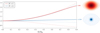Fig. 2. Mass growth in polytropes of indices N = 1 (red curves) and N = 3 (blue curves) as a function of the normalised rotation rate in the case of solid rotation. The upper and lower thin curves represent the equatorial and polar radii in both polytropes, respectively, and the thicker curves indicate their mass. All quantities are expressed in units of the non-rotating models’ parameters, and the percentages on the right side give the relative mass increase at Ω = 0.9ΩK with ${\mathrm{\Omega }}_{\text{K}}=\sqrt{\mathcal{G}M/R^3}$, the Keplerian rotation rate. The colour maps adjoining the curves depict the mass distribution in both models after deformation at Ω = 0.9ΩK.

In addition to the rotation rate, the amount of mass growth also depends on the initial mass distribution of the model, as illustrated in Fig. 2. Because the most deformed isopotentials are those located near the surface, models that concentrate most of the mass in their core (e.g., the polytrope of index N = 3) undergo an increase of only a few percent in their total mass, even at speeds close to the critical rotation rate. Conversely, more homogeneous models such as the N = 1 polytrope change significantly in mass because more mass is contained in these highly deformed isopotentials. In some cases, this can lead to a relative mass increase of over one-third.

3.3. Adaptive rotation rate

When going from one iteration to the next, we are faced with the following conundrum. The centrifugal potential depends on the value of rotation rate. It then subsequently intervenes in the total potential and hence the calculation of new isopotential surfaces. In particular, this leads to a new determination of the equatorial radius (which is generally larger than the previous estimate). However, this radius is required to obtain the rotation rate, which intervenes in the centrifugal potential, in order to ensure that the ratio Ω/Ω_K is preserved at the equator. Hence, the rotation rate and the equatorial radius are interdependent.

One may naively think that simply iterating the above algorithm, being a fixed-point scheme, will resolve this interdependence. However, if the (dimensionless) target rotation rate is sufficiently close to critical, then the critical rotation rate can easily be exceeded when the equatorial radius is updated. This then hampers calculating isopotential surfaces and thus causes the iterations to stop prematurely. In order to resolve this interdependence, we need to anticipate the value of the equatorial radius such that the target value of Ω/Ω_K is reached at the equator. For the sake of clarity, we now describe this using some equations. In what follows, the indices i and i + 1 refer to the current and following iteration, and the index ∞ denotes their limits. In order to avoid overloading an already cumbersome notation, dimensionless versions of the quantities R, Ω, Φ are denoted r, ω, ϕ, respectively.

From a mathematical point of view, the problem occurs when attempting to find an isopotential with a value Φ_eff > ${\mathrm{\Phi }}_{\text{eff}}^{ \text{crit}}$, the latter being defined as the value of the potential for which ∇Φ_eff ⋅ e_r = 0 on the equator. Figure 3 provides a clear view of what happens in this case: because these isopotentials are not closed surfaces, Newton’s method, as described in Sect. 2.3, cannot converge on the equator, and the algorithm simply breaks down. This issue might be surprising at first glance because it is clear that even the value of the highest isopotential (corresponding to the surface) should remain below ${\mathrm{\Phi }}_{\text{eff}}^{ \text{crit}}$ as long as the specified rotation profile, Ω(s), satisfies Ω_eq/Ω_K < 1.

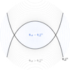Fig. 3. Typical shapes of isopotentials in a meridional cross section, inside and outside a rotating model. The critical isopotential (denoted by its value, ${\mathrm{\Phi }}_{\text{eff}}^{ \text{crit}}$) is shown in black, and the level surfaces with higher and lower values appear in grey and blue, respectively.

In a naive iterative scheme, however, it is possible to face this issue because the Keplerian break-up rotation rate, ${{\mathrm{\Omega }}_{\text{K}}}^i=\sqrt{\mathcal{G}{M}^i/{{R_{\text{eq}}}^i}^3}$, changes from one iteration to the next. Furthermore, because the equatorial radius increases faster than the mass as a function of the rotation rate (cf. Fig. 2), and because the dimensionless rotation rate on the equator ω_eq does not change, the final equatorial rotation rate ${\mathrm{\Omega }}_{\text{eq}}^{ \infty }={\omega }_{\text{eq}}{\mathrm{\Omega }}_{\text{K}}^{ \infty }$ is lower than the initial value, thus implying that it decreased at some point in the iterations. In other words, the determination of the outermost isopotential with the current equatorial rotation rate, ${\mathrm{\Omega }}_{\text{eq}}^{ i}$, might have a value exceeding ${\left({\mathrm{\Phi }}_{\text{eff}}^{ \text{crit}}\right)}^{ i+1}$ if ${\mathrm{\Omega }}_{\text{eq}}^{ i}/{\mathrm{\Omega }}_{\text{K}}^{ i+1}>1$. The closer ω_eq is to 1, the higher the likelihood that this problem occurs.

To overcome this difficulty, a new sequence of equatorial rotation rates, ${\stackrel{\sim }{\mathrm{\Omega }}}_{\mathrm{eq}}^i$, must be found such that the procedure finally converges towards ${\mathrm{\Omega }}_{\text{eq}}^{ \infty }={\omega }_{\text{eq}}{\mathrm{\Omega }}_{\text{K}}^{ \infty }$, without ever facing the criterion just stated above. The solution we found is to define this sequence as

$$\begin{array}{c}\hfill {\stackrel{\sim }{\mathrm{\Omega }}}_{\mathrm{eq}}^i={\omega }_{\mathrm{eq}}{\stackrel{\sim }{\mathrm{\Omega }}}_K^i,\end{array}$$(27)

where ${\stackrel{\sim }{\mathrm{\Omega }}}_K^i=\sqrt{\mathcal{G}{M}^i/{({R_{\text{eq}}}^{i+1})}^3}$. In terms of the current scaling, this solution amounts to adapting the dimensionless rotation rate during the iterations because ${\stackrel{\sim }{\mathrm{\Omega }}}_{\mathrm{eq}}^i$ can be re-expressed as

$$\begin{array}{c}\hfill {\stackrel{\sim }{\mathrm{\Omega }}}_{\mathrm{eq}}^i={\stackrel{\sim }{\omega }}_{\mathrm{eq}}^i{\mathrm{\Omega }}_{\mathrm{K}}^i,\end{array}$$(28)

with

$$\begin{array}{c}\hfill {\stackrel{\sim }{\omega }}_{\mathrm{eq}}^i={\omega }_{\mathrm{eq}}\frac{{\stackrel{\sim }{\mathrm{\Omega }}}_{\mathrm{K}}^i}{{\mathrm{\Omega }}_{\mathrm{K}}^i}={\omega }_{\mathrm{eq}}{(r_{\mathrm{eq}}^{i+1})}^{-3/2},\end{array}$$(29)

where $r_{\text{eq}}^{ i+1}$ denotes the next equatorial radius expressed in the current scaling, $R_{\text{eq}}^{ i+1}/R_{\text{eq}}^{ i}$. Because the mass tends to increase from one iteration to the next, we can easily check that ${\stackrel{\sim }{\mathrm{\Omega }}}_K^i<{{\mathrm{\Omega }}_{\text{K}}}^{i+1}$ and therefore that the sequence we define verifies

$$\begin{array}{c}\hfill \frac{{\stackrel{\sim }{\mathrm{\Omega }}}_{\mathrm{eq}}^i}{{\mathrm{\Omega }}_{\mathrm{K}}^{i+1}}={\stackrel{\sim }{\omega }}_{\mathrm{eq}}^i\frac{{\mathrm{\Omega }}_{\mathrm{K}}^i}{{\mathrm{\Omega }}_{\mathrm{K}}^{i+1}}={\omega }_{\mathrm{eq}}\frac{{\stackrel{\sim }{\mathrm{\Omega }}}_K^i}{{\mathrm{\Omega }}_{\mathrm{K}}^i}\frac{{\mathrm{\Omega }}_{\mathrm{K}}^i}{{\mathrm{\Omega }}_{\mathrm{K}}^{i+1}}<{\omega }_{\mathrm{eq}}<1\end{array}$$(30)

for a given iteration i. Moreover, as long as the sequence of equatorial radii converges towards a finite limit $R_{\text{eq}}^{ \infty }$, the ratio of successive radii converges towards, $r_{\text{eq}}^{ \infty }=1$, thus proving with Eq. (29) that the adaptive rotation rate we defined asymptotically approaches the user-specified value,

$$\begin{array}{c}\hfill \underset{i\to \infty }{lim}{\stackrel{\sim }{\omega }}_{\mathrm{eq}}^i={\omega }_{\mathrm{eq}}.\end{array}$$(31)

While this new definition seems to have all the desired properties (cf. Eqs. (30) and (31)), it must be noted that the latter requires the evaluation of $R_{\text{eq}}^{ i+1}$ at iteration i. Although anticipating the next equatorial radius is generally not possible in such an iterative procedure, an interesting feature in RUBIS enables calculating it exactly. Because the effective potential only varies by an additive constant from one iteration to the next (cf. Eq. (6)), it may be pointed out that the difference

$$\begin{array}{cc}& \delta \mathrm{\Phi }\equiv {\mathrm{\Phi }}_{\mathrm{eff}}(\zeta =1)-{\mathrm{\Phi }}_{\mathrm{eff}}(\zeta =0)\hfill \\ \hfill & ={\mathrm{\Phi }}_{\mathrm{G}}(R_{\mathrm{eq}},\pi /2)+{\mathrm{\Phi }}_{\mathrm{C}}(R_{\mathrm{eq}},\pi /2)-{\mathrm{\Phi }}_{\mathrm{G}}(0,\pi /2)\hfill \end{array}$$(32)

does not change. We note that the constant δΦ is known from the first iteration, after having solved Poisson’s equation. We now place ourselves at iteration i and try to anticipate the content of this equation at iteration i + 1. Scaled by the current reference potential $\mathcal{G}{M}^i/R_{\text{eq}}^{ i}$, the above equation becomes

$$\begin{array}{c}\hfill \delta {\varphi }^i={\varphi }_g(r_{\mathrm{eq}}^{i+1},\pi /2)-{\varphi }_g(0,\pi /2)-{\displaystyle {\int }_0^{r_{\mathrm{eq}}^{i+1}}x{[{\mathrm{\Omega }}^i(x{R}_{\mathrm{eq}}^i)/{\mathrm{\Omega }}_{\mathrm{K}}^i]}^2\mathrm{d}x,}\end{array}$$(33)

where we expressed the centrifugal potential using Eq. (3) and defined $\delta {\varphi }^i=\delta \mathrm{\Phi }\times {\left(\mathcal{G}{M}^i/R_{\text{eq}}^{ i}\right)}^{-1}$. In this equation, the scaled rotation profile Ωⁱ(s) depends on the iteration because its equatorial value changes with i (cf. Eq. (28)). The way the whole profile changes with its equatorial value in RUBIS can simply be described with the following scaling relation:

$$\begin{array}{c}\hfill {\mathrm{\Omega }}^i(s)={\stackrel{\sim }{\mathrm{\Omega }}}_{\mathrm{eq}}^i\times \overline{\omega }(s/R_{\mathrm{eq}}^i),\end{array}$$(34)

where $\overline{\omega }$ designates the dimensionless profile such that $\overline{\omega }(1)=1$. Injecting this expression into Eq. (33) and replacing ${\stackrel{\sim }{\mathrm{\Omega }}}_{\mathrm{eq}}^i/{{\mathrm{\Omega }}_{\text{K}}}^i$ using Eq. (29), we obtain

$$\begin{array}{c}\hfill \delta {\varphi }^i={\varphi }_g(r_{\mathrm{eq}}^{i+1},\pi /2)-{\varphi }_g(0,\pi /2)-\frac{{\omega }_{\mathrm{eq}}^2}{{(r_{\mathrm{eq}}^{i+1})}^3}{\displaystyle {\int }_0^{r_{\mathrm{eq}}^{i+1}}x{\overline{\omega }}^2(x)\mathrm{d}x.}\end{array}$$(35)

Rescaling the x variable in the integral so that it varies between 0 and 1, we deduce the final relation,

$$\begin{array}{c}\hfill \delta {\varphi }^i={\varphi }_g(r_{\mathrm{eq}}^{i+1},\pi /2)-{\varphi }_g(0,\pi /2)-\frac{\mathcal{R}{\omega }_{\mathrm{eq}}^2}{r_{\mathrm{eq}}^{i+1}},\end{array}$$(36)

with ℛ a constant fixed by the choice of the rotation profile,

$$\begin{array}{c}\hfill \mathcal{R}={\displaystyle {\int }_0^1}x{\overline{\omega }}^2(x)\mathrm{d}x.\end{array}$$(37)

For instance, the choice of a uniform rotation profile leads to $\overline{\omega }(x)=1$ and thus ℛ = 1/2, while choosing a Lorentzian profile (cf. Eq. (22)) yields

$$\begin{array}{c}\hfill \overline{\omega }(x)=\frac{1+\alpha }{1+\alpha x^2}\Rightarrow \mathcal{R}=\frac{1+\alpha }{2}.\end{array}$$(38)

Equation (36) is merely an equation of the type $f(r_{\text{eq}}^{ i+1})=\delta {\varphi }^i$ which can be solved numerically for $r_{\text{eq}}^{ i+1}$ using Newton’s method and noting that

$$\begin{array}{c}\hfill \frac{\mathrm{d}f}{\mathrm{d}r}={\frac{\partial {\varphi }_g}{\partial r}|}_{\theta =\pi /2}+\mathcal{R}{\left(\frac{{\omega }_{\mathrm{eq}}}{r}\right)}^2\end{array}$$(39)

is known. Once $r_{\text{eq}}^{ i+1}$ is found, the adaptive rotation rate follows immediately from Eq. (29).

In practice, this modification has a negligible numerical cost, but offers a substantial gain in performance, both in terms of stability and convergence speed. Figure 4 quantifies the benefits of this modification to the program by comparing the number of iterations required for convergence in the fixed and adaptive rotation rate approaches. While the first method requires more and more iterations as Ω increases and finally does not converge beyond 0.8Ω_K, the adaptive approach reaches the desired criterion in a quasi-constant number of steps (about 25) regardless of the rotation speed.

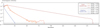Fig. 4. Number of iterations needed to reach the convergence criterion (in this case |(Rpol/Req)i + 1−(Rpol/Req)i| < 10−11) for the fixed rotation rate approach (red hue curves) and adaptive method (blue tint curves) presented in Sect. 3.3 (the radial and angular resolutions chosen were N = 1000 and L = 101, respectively). For each approach, the degree of convergence as a function of iteration number is shown for three rotation rates. In the fixed-rotation approach, a transient phase in which the rotation speed gradually increases must be included at the beginning. In the case of the adaptive method, the three curves overlap.

In terms of stability, it is possible to reach speeds that are extremely close to the critical rotation rate. Figure 5 shows the cross section of an N = 3 polytrope at Ω = 0.9999Ω_K. At this speed, the last isopotential approaches the saddle point very closely thus leading to a well-defined cusp at the equator. A high truncation order is required (L = 500) in order to properly resolve this region.

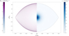Fig. 5. Deformation of an N = 3 polytrope at 99.99% of the critical rotation rate. The left side of the figure shows the shape of the level surfaces and their colour reflects the value of the effective potential. The right side shows the mass distribution in the model.

4. Tests

As was pointed out in previous sections, the method developed here preserves the polytropic relation between ρ and P. We hereafter compare the deformations and structures obtained using the present method, and in some cases, the resultant pulsation modes, with those generated by independent methods, namely the approaches developed in Rieutord et al. (2005), in the ESTER code (Espinosa Lara & Rieutord 2013; Rieutord et al. 2016), and in the Concentric MacLaurin Spheroids (CMS) method (Hubbard 2012, 2013).

4.1. Polytropes

A particularly relevant and well-studied class of models to test are polytropes. Indeed, polytropes with indices of N = 1.5 and 3 have been used as a first approximations of convective and radiative regions in stars (e.g., Eddington 1926; Chandrasekhar 1939), while an index of 1 has been used to model the envelope of planetary models such as Jupiter (e.g., Stevenson 1982). Furthermore, the pulsation modes of such models have been calculated to a great accuracy by various authors (Christensen-Dalsgaard & Mullan 1994; Lignières et al. 2006; Reese et al. 2006; Ballot et al. 2010) and may be used as reference to test new methods. In addition to this, rotating polytropes preserve their barotropic relation, so that the central assumption of the present method is exactly verified for these particular models. Therefore, very small differences are expected compared to other deformation methods.

The polytropes generated using the present method have a uniform radial grid with 1001 points and a colatitude grid of 101 points distributed along a Gauss-Legendre collocation grid. The models generated using the Rieutord et al. (2005) method are discretised using spectral methods in both the radial and latitudinal directions. A resolution of 81 points was used in the radial direction and 51 spherical harmonics (with even ℓ values ranging from 0 to 100) for the horizontal structure.

In order to account for the differences between the two methods, we chose to compare the positions of the level surfaces in a fast-rotating N = 3 polytrope. More specifically, we considered a uniform rotation at rate of 0.8Ω_K. This meant interpolating the Rieutord et al. (2005) model to find the 1001 corresponding level surfaces as it is initially calculated using a mapping based on Bonazzola et al. (1998). Figure 6 shows the result of this comparison, that is, the value of the differences

$$\begin{array}{c}\hfill \delta r(\zeta ,\theta )=r^{\mathrm{R}05}(\zeta ,\theta )-r^{\mathrm{RUBIS}}(\zeta ,\theta )\end{array}$$(40)

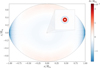Fig. 6. Differences on level surfaces of the 0.8ΩK polytropic models. The mappings were again normalised by the equatorial radius. The inset centred on the origin, where the differences are the greatest, is only 0.01Req wide.

inside the deformed models. The maximum differences are about 10⁻⁹, and, in most of the model, they are well below this value, thus confirming the excellent agreement of the two methods. The most central (and pronounced) differences here are the result of the solving method used for Poisson’s equation. In RUBIS, this equation is solved on r² rather than r for regularity purposes, which may explain the 10⁻⁹ variations in Φ_G in this region, although the deformation is very small in practice.

One of the goals of the method presented here is to produce models that may be used for accurate pulsation calculations. We therefore compared the pulsation frequencies of the most rapidly rotating model from Reese et al. (2006), that is, an N = 3 polytrope rotating at Ω = 0.58946223Ω_K generated using the Rieutord et al. (2005) method, with those of an equivalent model produced with the present method. This time, we increased the radial resolution of the model with the present method to n = 2000 points using an unevenly spaced grid. The successive ζ positions (or r positions of the precursor 1D model) are given by

$$\begin{array}{c}\hfill {\zeta }_i=sin\left(\frac{(i-1)\pi }{2(n-1)}\right),1\le i\le n.\end{array}$$(41)

This grid has a roughly uniform spacing of $\sim \frac{\pi }{2n}$ around ζ = 0 and a dense spacing that scales as 1/n² near ζ = 1, thus making it suitable for p-mode calculations. Figure 7 show the relative frequency differences between the two models. These differences are about 10⁻⁷, except for the lowest-frequency modes, thus confirming that the present method is fully able to produce accurate models that are suitable for seismic calculations.

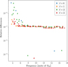Fig. 7. Relative frequency differences between pulsation calculations in the N = 3, Ω = 0.58946223ΩK polytrope from Reese et al. (2006) and an equivalent model from the present method as a function of the oscillation frequency (expressed in units of the Keplerian rotation rate, ΩK). The different colours indicate the harmonic degree of the oscillation modes that are carried over from the non-rotating case. All azimuthal orders (|m|≤ℓ) are provided for each degree.

4.2. ESTER models

While RUBIS has been shown to reliably reproduce the structure of 2D polytropic models, its underlying assumptions suggest that the same cannot be said for more realistic structures. This is evaluated in this section. In particular, we compare structures derived from RUBIS and those derived from the ESTER code, which satisfy an energy balance in addition to the hydrostatic equilibrium. However, before this, we first make use of ESTER to verify the relevance of RUBIS’ central assumption, namely the conservation of the barotropic relation during the deformation process. To this end, we compared the relation between the density and pressure in a rotating star obtained with ESTER and its non-rotating equivalent. However, there is an important aspect to consider in order to do this accurately. It was mentioned earlier that a deformation that preserves the barotropic relation does not conserve the mass of the model for the simple reason that its volume increases. Thus, it is to be expected that the density values in models of the same mass with and without rotation are not directly comparable. More precisely, the non-rotating model should be denser because its volume is smaller. This apparent problem can readily be solved: rather than comparing a rotating model with a static model of the same mass, one simply needs to compare it with the model that will have the same mass after a deformation that preserves ρ(P), that is, deformed with RUBIS. Here, the difficulty arises from the impossibility of imposing the same rotation profile, RUBIS being limited to conservative rotation profiles, whereas the ESTER profiles are fully differential (i.e. non-conservative). To account for the change in mass, at least partly, we compared an ESTER model with a model that reaches the same mass after having been deformed using a uniform rotation profile with $\mathrm{\Omega }={\mathrm{\Omega }}_{\text{eq}}^{\text{ESTER}}$, where ${\mathrm{\Omega }}_{\text{eq}}^{\text{ESTER}}$ is the equatorial rotation rate from ESTER. Most of the deformation should be taken into account in this way, although the differences δΩ between the two rotation profiles are part of the limitations to be kept in mind. This is confirmed by the relatively small difference in flattening between the two models (cf. Table 3). Nonetheless, larger differences remain on the polar and equatorial radii, thus affecting the Keplerian break-up rotation rate, as also shown in Table 3.

In Fig. 8 we compare the pairs (ρ, P) from a 2 M_⊙ ESTER model with a differential rotation verifying ${\mathrm{\Omega }}_{\text{eq}}^{\text{ESTER}}$ = 0.8Ω_K with the relation ρ(P) from a 1D model of mass 1.977127 M_⊙. When deformed by RUBIS using a uniform rotation profile with Ω = 0.8Ω_K, the latter leads to a 2 M_⊙ model that by construction verifies the same relation between density and pressure. In Fig. 8 two major properties stand out. First, although there is no relation in the functional sense between ρ and P in the model deformed by ESTER, all pairs (ρ, P) seem to align on the same curve. A high zoom level is necessary to reveal some thickness in this point distribution, resulting from angular differences. It thus highlights the relevance of assuming the existence of such a relation even to approximate more realistic cases, where energy transfer is taken into account. Moreover, this relation does not seem to be just any relation: the (ρ, P) pairs almost perfectly overlap with the ρ(P) relation of the non-rotating model. This observation is central and constitutes a major motivation for developing a code such as RUBIS. A closer inspection of the two structures reveals some differences, as we discuss below.

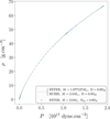Fig. 8. Comparison of the 1D relation ρ(P) in a 1.977127 M⊙ star without rotation (grey curve) and the pairs (ρ, P) from a 2 M⊙ star obtained by ESTER using a differential rotation profile, the equatorial speed of which is Ωeq = 0.8ΩK (blue dots). The brackets indicate that the relation ρ(P) shown here for the 1D model also corresponds to the relation in the model deformed by RUBIS using the uniform rotation speed Ω = 0.8ΩK (the mass of the model then reaches 2 M⊙).

A drawback of Fig. 8 is that it does not reveal the regions of the star in which potential structural differences may arise. In order to compare the structures, they need to be interpolated to the same pressure values⁸, the problem being that the methods used by ESTER and RUBIS do not use the same convention when defining the pseudo-radial variable, ζ. To do this, it is first necessary to interpolate the pressure as a function of ζ and θ in the ESTER model using the fact that it is defined on a multi-domain Gauss-Lobatto grid. We then find at which pairs (ζ^ESTER, θ) the pressure values in the RUBIS model correspond, keeping in mind that the latter are defined at a fixed ζ^RUBIS. We now interpolate the ESTER density in order to evaluate it at (ζ^ESTER, θ) and we define

$$\begin{array}{c}\hfill {\delta }_P\rho ({\zeta }^{\mathrm{RUBIS}})=\rho ({\zeta }^{\mathrm{RUBIS}})-\rho ({\zeta }^{\mathrm{ESTER}},\theta ).\end{array}$$(42)

Here, the notation δ_P indicates a difference at fixed pressure value, more specifically, the one that is found at ζ^RUBIS. The quantity δ_Pρ therefore contains the deviations from barotropy obtained in the ESTER model, deviations that can be located physically. We note that it also possible to define normalised differences, δ_Pρ/ρ, which are represented along with δ_Pρ in Fig. 9.

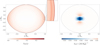Fig. 9. Relative and absolute density differences between RUBIS and ESTER. Left panel: relative density differences between the models computed with RUBIS and ESTER at given pressure values. The latter are placed according to the position in which these pressure values are met in the RUBIS deformation. The zoomed-in frame helps to reveal the differences in the most superficial layers at the equator. Right panel: same as the left panel, but for the absolute differences in density (expressed this time in units of $M/R_{\text{eq}}^3$.

The figure shows that the normalised differences remain below 1% in the innermost half of the star. However, they rapidly increase near the surface, eventually reaching 10% in the ionisation region (on the equator), which is reflected in the red stripe in the zoomed-in frame. The largest relative differences exceed one-third and are located in the most superficial layers of the model (dark red curve around the star).

The absolute differences, on the other hand, offer an alternative picture. Near the centre, where we find nearly solid rotation, the differences first take the form of a nearly spherical function. Beyond a certain layer, however, these differences exhibit angular variations and reflect a more general differential rotation in the ESTER model. The absolute differences then rapidly tend towards 0.

These differences can mainly be attributed to two factors. First, as mentioned above, the two models do not have the same rotation profile. Some of these differences might be taken into account by defining a best-fitting conservative profile as

$$\begin{array}{c}\hfill \mathrm{\Omega }(s)=\frac{{\int }_0^{Z(s)}\rho {\mathrm{\Omega }}^{\mathrm{ESTER}}(z,s)\mathrm{d}z}{{\int }_0^{Z(s)}\rho (z,s)\mathrm{d}z},\end{array}$$(43)

with Z(s) the position of the surface at a distance s from the rotation axis. However, this factor alone does not explain all of the observed differences, and we can also expect that the thermal structure, verifying a more complex equilibrium in the ESTER model, is only approximately reproduced by a model deformed with RUBIS. Although the hydrostatic and thermal structures can be seen as uncorrelated as long as the equation of state is not specified, in the sense that an infinite number of thermal structures and equations of state can lead to the same equilibrium, it is obviously not the case for a model aiming to verify an energy transfer equilibrium. We can therefore expect such differences between RUBIS and ESTER.

In practice, the two representations given in Fig. 9 have their own relevance depending on the model’s usage. For example, the high relative differences on the surface can be expected to play an important role when calculating high-degree pressure modes. On the other hand, gravity modes or global quantities sensitive to mass distribution such as gravitational moments may be more sensitive to the second representation.

In the following, we account for the impact of these differences on the oscillation frequencies of the models. Using the Two-dimensional Oscillation Program (TOP; Reese et al. 2006, 2009), we computed and identified the oscillation modes corresponding to the $\stackrel{\sim }{\ell }=0,1$, $\stackrel{\sim }{n}=9,23$ acoustic island modes. We recall that island modes are the rotating counterparts to low-degree acoustic modes. They focus on a period ray orbit that circumvents the equator. The quantum number $\stackrel{\sim }{n}$ corresponds to the number of nodes along the orbit’s path whereas $\stackrel{\sim }{\ell }$ is the number of nodes parallel to the orbit (cf. Lignières & Georgeot 2008; Reese 2008; and Pasek et al. 2012 for a more detailed definition of $\stackrel{\sim }{\ell }$ and $\stackrel{\sim }{n}$ and their link with usual spherical quantum numbers). The frequency differences, δω, defined as

$$\begin{array}{c}\hfill \delta \omega ={\omega }^{\mathrm{ESTER}}-{\omega }^{\mathrm{RUBIS}},\end{array}$$(44)

are represented in the upper panel of Fig. 10 as a function of the azimuthal order m for the $\stackrel{\sim }{\ell }=0$ and $\stackrel{\sim }{\ell }=1$ oscillation modes.

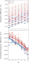Fig. 10. Frequency differences in μHz (upper panel), as defined in Eq. (44), along with their normalised counterparts (lower panel) introduced in Eq. (45). These differences are shown as a function of the azimuthal order, m, for the $\stackrel{\sim }{\ell }=0$ (blue shades) and $\stackrel{\sim }{\ell }=1$ (red shades) island modes. The colour shade indicates the mode’s pseudo-radial order, $\stackrel{\sim }{n}$ (higher orders correspond to darker colours).

The first point to highlight is that the differences are not distributed around zero, but exhibit a clear negative offset. The reason for this is the different frequency scales resulting from the differences in radii (cf. Table 3). This is confirmed by the fact that the differences increase with $\stackrel{\sim }{n}$, as indicated by the colour shades in Fig. 10. It also explains the trend as a function of the azimuthal order m. Indeed, in our convention, modes with negative m values are prograde and therefore have higher frequencies. This then highlights the difference in frequency scale.

When we now normalise the frequencies to account for these scaling effects as well as for the order of magnitude of the frequency differences, we obtain the differences shown in the lower panel of Fig. 10. These differences may be expressed as follows:

$$\begin{array}{c}\hfill \frac{\delta \sigma }{\sigma }=[\frac{{\omega }^{\mathrm{ESTER}}}{{\mathrm{\Omega }}_{\mathrm{K}}^{\mathrm{ESTER}}}-\frac{{\omega }^{\mathrm{RUBIS}}}{{\mathrm{\Omega }}_{\mathrm{K}}^{\mathrm{RUBIS}}}]{\left(\frac{{\omega }^{\mathrm{ESTER}}}{{\mathrm{\Omega }}_{\mathrm{K}}^{\mathrm{ESTER}}}\right)}^{-1}.\end{array}$$(45)

The negative offset has mostly been removed, along with the previously observed trend with $\stackrel{\sim }{n}$. This representation also reveals that the normalised frequency differences are of a few thousandths. They are considerably higher than in the case of a comparison between barotropic models with the same rotation profiles (cf. Fig. 7).

It is also interesting to note that the trend as a function of m has been reversed. Indeed, by removing the scaling effects, this highlights more subtle effects that are related to the rotation profiles of the two models, as we now explain. Following Reese et al. (2021), the rotational splittings in ESTER can be expressed (neglecting the Coriolis force) as

$$\begin{array}{c}\hfill {\omega }_{-m}-{\omega }_{+m}\simeq 2m{\mathrm{\Omega }}_{\mathrm{eff}},\end{array}$$(46)

where

$$\begin{array}{c}\hfill {\mathrm{\Omega }}_{\mathrm{eff}}={\displaystyle {\int }_V\mathrm{\Omega }(r,\theta )\mathcal{K}(r,\theta )\mathrm{d}V,}\end{array}$$(47)

is a weighted average of Ω, and 𝒦 is a (mode-dependent) rotation kernel, defined as

$$\begin{array}{c}\hfill \mathcal{K}(r,\theta )=\frac{1}{2}[\frac{\rho |{\mathbf{\xi }}_{+m}{|}^2}{{\displaystyle {\int }_V\rho {|{\mathbf{\xi }}_{+m}|}^2\mathrm{d}V}}+\frac{\rho |{\mathbf{\xi }}_{-m}{|}^2}{{\displaystyle {\int }_V\rho {|{\mathbf{\xi }}_{-m}|}^2\mathrm{d}V}}],\end{array}$$(48)

where |ξ_±m| designates the retrograde (+m) (or prograde (−m)) mode amplitude.

Because the rotation profile is differential in the ESTER model, the value of Ω_eff is likely to differ from Ω_eq. Moreover, because Ω(r, θ) tends to be higher than Ω_eq in the regions probed by 𝒦(r, θ), it is to be expected that

$$\begin{array}{c}\hfill {\omega }_{+m}-{\omega }_{-m}>2m{\mathrm{\Omega }}_{\mathrm{eq}},\end{array}$$(49)

where we made use of Eq. (46). In contrast, the model deformed by RUBIS rotates uniformly, thus leading to

$$\begin{array}{c}\hfill {\omega }_{+m}-{\omega }_{-m}\simeq 2m{\mathrm{\Omega }}_{\mathrm{eq}}.\end{array}$$(50)

By comparing the non-dimensional version of the two above equations, and recalling that the non-dimensional equatorial rotation rate is the same in both models, we obtain

$$\begin{array}{c}\hfill \delta ({\sigma }_{-m}-{\sigma }_m)\simeq 2m\delta {\mathrm{\Omega }}_{\mathrm{eff}}/{\mathrm{\Omega }}_{\mathrm{K}},\end{array}$$(51)

where

$$\begin{array}{c}\hfill \delta {\mathrm{\Omega }}_{\mathrm{eff}}={\displaystyle {\int }_V(\mathrm{\Omega }(r,\theta )-{\mathrm{\Omega }}_{\mathrm{eq}})\mathcal{K}(r,\theta )\mathrm{d}V>0.}\end{array}$$(52)

Regarding the structure of the modes themselves, we compare in Fig. 11 the following oscillation modes obtained in the RUBIS and ESTER models: $(\stackrel{\sim }{n},\stackrel{\sim }{l},m)=(13,1,2)$ and (13, 0, 1) (cf. upper and lower panels). The first comparison shows a typical example of a mode that is almost identical in the RUBIS and ESTER models, and the second comparison exhibits clear differences in the two modes. More specifically the mode in the ESTER model is considerably altered by an avoided crossing, while its impact is just beginning to emerge in its counterpart in the RUBIS model. Overall, the oscillation modes that possess well-defined structures are very similar, and even some avoided crossings are well reproduced in both models.

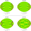Fig. 11. Two oscillation modes (upper and lower parts of the figure) in the RUBIS and ESTER models (left and right sides). The mode at the top is an $\stackrel{\sim }{\ell }=1$, m = 2 antisymmetric (with respect to the equator) mode, and the mode at the bottom corresponds to $\stackrel{\sim }{\ell }=0$, m = 1. The oscillation frequency of each mode is indicated in units of ΩK.

4.3. Model of Jupiter

To illustrate the capabilities of RUBIS in deforming planetary models, we considered the centrifugal deformation of a model of Jupiter. This specific case is very interesting in practice, whether to determine Jupiter’s structure by fitting its gravitational moments (Hubbard 2012, 2013; Debras & Chabrier 2018) or to interpret oscillation modes obtained through projects following the Jovian Oscillations through Velocity Images At several Longitudes (JOVIAL) project (Gonçalves et al. 2019).

In order to illustrate the capabilities of RUBIS in deforming planetary models, we considered a Jupiter model provided by the Code d’Evolution Planetaire Adaptatif et Modulaire (CEPAM; Guillot & Morel 1995). This model presents a strong density discontinuity due to the presence of a solid core (causing a change of ∼75% in density), making it an ideal application to test the program’s stability. In Fig. 12 we represent the mass distribution in the Jovian model when imposing a solid rotation rate of Ω ≃ 0.298656Ω_K, which corresponds to the rotation rate used in Debras & Chabrier (2018). The most central discontinuity, which corresponds to the solid core, is clearly visible in the colour change. A more discrete discontinuity caused by the metallic to molecular phase change in the envelope is highlighted with a white contour. Finally, the code continues to converge even for Jovian models exceeding 0.9Ω_K, although their concrete applications become somewhat uncertain.

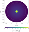Fig. 12. Mass distribution in a Jovian model after imposing a uniform rotation at Ω ≃ 0.298656ΩK using RUBIS. The white contours indicate the location of the model’s discontinuities.

Another advantage of using RUBIS for deforming planetary models lies in the excellent accuracy it provides at a very low numerical cost. This is illustrated here through a classic problem of Jovian science: the calculation of gravitational moments able to satisfy the observational constraints of Juno. Based on numerous flybys of the planet (Bolton et al. 2017), the probe is able to provide very reliable estimates of Jupiter’s gravitational moments (cf. Table 4), defined as

$$\begin{array}{c}\hfill J_{\ell }=-\frac{1}{M{R}_{\mathrm{eq}}^{\ell }}{\displaystyle {\int }_V{r}^{\ell }\rho (r,\theta )P_{\ell }(cos\theta )\mathrm{d}V,}\end{array}$$(53)

where P_ℓ designates the ℓth Legendre polynomial, and therefore to account for the departures from a spherically symmetric matter distribution caused by the rotation.

However, a considerable difficulty in comparing these observational values with those of Jovian models is the accuracy that deformation codes can achieve for these moments. A classic benchmark to test this is the calculation of the gravitational moments of the N = 1 polytrope with the deformation parameter q = ω² = 0.089195487 because they can be calculated analytically. We provide in Table 5 a comparison of these analytical values and the numerical estimates from several methods: the Theory of Figure (ToF) to order q³, the CMS method using 512 spheroids, and the method presented here. The studies from which these values are taken can be found below the table. We facilitate the comparison between columns by indicating in red the digits that do not match the analytical values.

In order to reach an optimal accuracy, we used a radial grid of 10 000 points with a Gauss-Legendre grid of 101 points in the angular direction for a maximum harmonic degree L of 100. Numerical errors on the moments were assessed via the variance resulting from more than 100 runs with slight variations in the radial grid. Digits that are correct on average but may change between runs are indicated in grey in Table 5.

The results are quite impressive. Whereas the ToF method leads to an absolute error of about 10⁻⁵ − 10⁻⁶ and the CMS method has a relative error of 10⁻⁴, RUBIS exhibits an absolute error of about 10⁻¹³ that is reduced to 10⁻¹⁴ − 10⁻¹⁶ when considering the average estimates. Moreover, this accuracy can be achieved at a fairly low numerical cost. For instance, the RUBIS deformation process described here was performed using a 1.9 GHz Intel Core i7-8665U CPU with four-cores (eight-threads) processor, running in 33.9 s on average and requiring 4.1 GB of memory.

Finally, we emphasise that, compared to other methods such as the Consistent Level Curves (CLC) method, which can achieve arbitrarily high accuracy on the moments (Wisdom & Hubbard 2016), RUBIS was designed to be able to take into account density discontinuities in a consistent manner. Its ability to overcome the difficulties faced by CMS when increasing the number of spheroids (Debras & Chabrier 2018) and thus guarantee very high accuracy even for the first moments makes it a reasonable choice when searching for Jovian models subject to the constraints of Juno.

5. Conclusion

We presented RUBIS, a fully Python-based centrifugal deformation program that can be accessed from this GitHub repository⁹. The program takes in an input 1D (spherically symmetric) model and returns its deformed counterpart by applying a conservative rotation profile specified by the user. More specifically, the code only needs the density profile as a function of radial distance, ρ(r), from the reference model in addition to the surface pressure, P₀, in order to perform the deformation. The program is particularly lightweight because of the central assumption, which consists in preserving the relation between density and pressure when going from the 1D to the 2D structure. The latter makes it possible, in particular, to avoid the standard complications arising from energy conservation in the resulting model (Jackson 1970; Roxburgh 2004; Jackson et al. 2005; MacGregor et al. 2007). In this sense, the method is analogous to the one presented by Roxburgh (2006), but it is simpler because it does not require the calculation of the first adiabatic exponent, Γ₁, during the deformation process, thus bypassing the need to explicitly specify an equation of state.

As a result, the only equation solved by the program in practice is Poisson’s equation, ΔΦ_G = 4π𝒢ρ, thereby leading to very fast computation times even when high angular accuracy is required, thus making it a potentially valuable tool for multidimensional evolutionary applications. Another feature of the method is its excellent stability, which enables the deformation of models at speeds very close to the critical rotation rate. Finally, the code was designed to allow both stellar and planetary models to be deformed by dealing with potential discontinuities in the density profile. This is made possible by solving Poisson’s equation in spheroidal rather than spherical coordinates whenever a discontinuity is present.

By design, RUBIS is able to reach a high degree of accuracy when deforming polytropic structures, making them well suited to the calculation of oscillation frequencies. We also showed that the centrifugal deformations derived from RUBIS keep a certain degree of relevance even when approximating more complex baroclinic structures, and this even when they exhibit a differential rather than conservative rotation profile. Although observationally significant differences appear when comparing pulsation frequencies from RUBIS models with those of more realistic models, they nonetheless remain accurate to a few tenths of a percent when scaling effects have been taking into account. This is useful for providing a first estimate of stellar parameters when interpreting observed pulsation spectra, which can then guide more costly searches using more realistic models. Finally, we also demonstrated the ability of the program to deform discontinuous structures such as planetary models and illustrated its accuracy when calculating gravitational moments. The results are promising compared to the existing alternatives and highlight the viability of RUBIS as a model adjustment tool for fitting the measurements coming from the Juno probe.

Acknowledgments

The authors thank the referee for their comprehensive reading and very detailed comments which significantly contributed to making the article clearer. PSH and DRR warmly thank Pr. Tristan Guillot for providing them with a model of Jupiter which is deformed for illustrative purposes in Fig. 12. PSH and DRR acknowledge the support of the French Agence Nationale de la Recherche (ANR) to the ESRR project under grant ANR-16-CE31-0007 as well as financial support from the Programme National de Physique Stellaire (PNPS) of the CNRS/INSU co-funded by the CEA and the CNES. DRR also acknowledges the support of the ANR to the MASSIF project under grant ANR-21-CE31-0018-03.

References

Appendix A: Poisson’s equation and derivation of the interface conditions in spheroidal coordinates

We briefly retrace the derivation of Eq. (20) as well as the boundary conditions (A.11) and (A.18), while clarifying the notations associated with the coupling integrals ${\mathcal{P}}_{··}^{\ell \ell \prime }$. First of all, Eq. (18) can quickly be retrieved using the fact that ΔΦ_G = ∇ ⋅ ∇Φ_G, which in curvilinear coordinates is written as (using Einstein’s summation convention)

$$\begin{array}{c}\hfill \mathrm{\Delta }{\mathrm{\Phi }}_{\mathrm{G}}=\frac{{\partial }_i\left(\sqrt{|g|}{\partial }^i{\mathrm{\Phi }}_{\mathrm{G}}\right)}{\sqrt{|g|}}=\frac{{\partial }_i\left(g^{\mathit{ij}}\sqrt{|g|}{\partial }_j{\mathrm{\Phi }}_{\mathrm{G}}\right)}{\sqrt{|g|}}.\end{array}$$(A.1)

Here, g^ij denotes the covariant components of the metric tensor, and g is its determinant. Since ∂_φΦ_G = 0, the only components needed are $g^{\zeta \zeta }=(r^2+r_{\theta }{}^2){(r^2{r}_{\zeta }{}^2)}^{-1}$, g^ζθ = g^θζ = −r_θ(r²r_ζ)⁻¹ and g^θθ = r⁻², in addition to $g=r^4{r}_{\zeta }{}^2{sin}^2\theta$. Multiplying by r²r_ζ, the sum then results in four terms

$$\begin{array}{c}\hfill \begin{array}{cc}\hfill r^2{r}_{\zeta }\mathrm{\Delta }{\mathrm{\Phi }}_{\mathrm{G}}=& {\partial }_{\zeta }\left(\frac{r^2+r_{\theta }^2}{r_{\zeta }}{\partial }_{\zeta }{\mathrm{\Phi }}_{\mathrm{G}}\right)-{\partial }_{\zeta }\left(r_{\theta }{\partial }_{\theta }{\mathrm{\Phi }}_{\mathrm{G}}\right)\hfill \\ \hfill & -\frac{1}{sin\theta }{\partial }_{\theta }(r_{\theta }sin\theta {\partial }_{\zeta }{\mathrm{\Phi }}_{\mathrm{G}})+\frac{1}{sin\theta }{\partial }_{\theta }(r_{\zeta }sin\theta {\partial }_{\theta }{\mathrm{\Phi }}_{\mathrm{G}}).\hfill \end{array}\end{array}$$(A.2)

Expanding the last three terms and replacing ΔΦ_G by its actual value according to Poisson’s equation, 4π𝒢ρ, leads to

$$\begin{array}{c}\hfill {\partial }_{\zeta }\left(\frac{r^2+r_{\theta }^2}{r_{\zeta }}{\partial }_{\zeta }{\mathrm{\Phi }}_{\mathrm{G}}\right)-2r_{\theta }{\partial }_{\zeta \theta }^2{\mathrm{\Phi }}_{\mathrm{G}}-{\mathrm{\Delta }}_{\mathcal{S}}r{\partial }_{\zeta }{\mathrm{\Phi }}_{\mathrm{G}}+r_{\zeta }{\mathrm{\Delta }}_{\mathcal{S}}{\mathrm{\Phi }}_{\mathrm{G}}=4\pi \mathcal{G}{r}^2{r}_{\zeta }\rho ,\end{array}$$(A.3)

with ${\mathrm{\Delta }}_{\mathcal{S}}\equiv {sin}^{-1}\theta {\partial }_{\theta }\left(sin\theta {\partial }_{\theta }\right)={\partial }_{\theta \theta }^2+cot\theta {\partial }_{\theta }$. We recognise Eq. (18). Decomposing the gravitational potential over the (normal) Legendre polynomials,

$$\begin{array}{c}\hfill {\mathrm{\Phi }}_{\mathrm{G}}(\zeta ,\theta )={\displaystyle \sum _{{\ell }^{\prime }=0}^{\infty }}{\mathrm{\Phi }}_{\mathrm{G}}^{{\ell }^{\prime }}(\zeta )P_{{\ell }^{\prime }}(cos\theta ),\end{array}$$(A.4)

we now obtain

$$\begin{array}{c}\hfill \begin{array}{cc}\hfill {\displaystyle \sum _{{\ell }^{\prime }=0}^{\infty }}& {\partial }_{\zeta }\left(\frac{r^2+r_{\theta }^2}{r_{\zeta }}{P}_{{\ell }^{\prime }}{\partial }_{\zeta }{\mathrm{\Phi }}_{\mathrm{G}}^{{\ell }^{\prime }}\right)\hfill \\ \hfill & -[2r_{\theta }{\partial }_{\theta }{P}_{{\ell }^{\prime }}+{\mathrm{\Delta }}_{\mathcal{S}}r{P}_{{\ell }^{\prime }}]{\partial }_{\zeta }{\mathrm{\Phi }}_{\mathrm{G}}^{{\ell }^{\prime }}\hfill \\ \hfill & -{\ell }^{\prime }({\ell }^{\prime }+1)r_{\zeta }{P}_{{\ell }^{\prime }}{\mathrm{\Phi }}_{\mathrm{G}}^{{\ell }^{\prime }}=4\pi \mathcal{G}{r}^2{r}_{\zeta }\rho \hfill \end{array}\end{array}$$(A.5)

using the fact that Δ_𝒮P_ℓ = −ℓ(ℓ+1)P_ℓ.

Since ${\int }_{-1}^{-1}{P}_{\ell }(\mu )P_{\ell \prime }(\mu )d\mu ={\delta }_{\ell \ell \prime }$, we can project this equation onto the ℓth polynomial, which leads to

$$\begin{array}{c}\hfill {\displaystyle \sum _{{\ell }^{\prime }=0}^L{\partial }_{\zeta }\left({\mathcal{P}}_{\zeta \zeta }^{\ell {\ell }^{\prime }}{\partial }_{\zeta }{\mathrm{\Phi }}_{\mathrm{G}}^{{\ell }^{\prime }}\right)-{\mathcal{P}}_{\zeta \theta }^{\ell {\ell }^{\prime }}{\partial }_{\zeta }{\mathrm{\Phi }}_{\mathrm{G}}^{{\ell }^{\prime }}-{\mathcal{P}}_{\theta \theta }^{\ell {\ell }^{\prime }}{\mathrm{\Phi }}_{\mathrm{G}}^{{\ell }^{\prime }}=4\pi \mathcal{G}{(r^2{r}_{\zeta })}_{\ell }\rho }\end{array}$$(A.6)

by introducing the coupling integrals,

$$\begin{array}{cc}\hfill {\mathcal{P}}_{\zeta \zeta }^{\ell {\ell }^{\prime }}& ={\displaystyle {\int }_{-1}^1\frac{r^2+r_{\theta }^2}{r_{\zeta }}{P}_{\ell }{P}_{{\ell }^{\prime }}d(cos\theta ),}\hfill \end{array}$$(A.7)

$$\begin{array}{cc}\hfill {\mathcal{P}}_{\zeta \theta }^{\ell {\ell }^{\prime }}& ={\displaystyle {\int }_{-1}^1[2r_{\theta }{P}_{\ell }{\partial }_{\theta }{P}_{{\ell }^{\prime }}+{\mathrm{\Delta }}_{\mathcal{S}}r{P}_{\ell }{P}_{{\ell }^{\prime }}]d(cos\theta ),}\hfill \end{array}$$(A.8)

$$\begin{array}{cc}\hfill {\mathcal{P}}_{\theta \theta }^{\ell {\ell }^{\prime }}& ={\ell }^{\prime }({\ell }^{\prime }+1){\displaystyle {\int }_{-1}^1{r}_{\zeta }{P}_{\ell }{P}_{{\ell }^{\prime }}d(cos\theta )}\hfill \end{array}$$(A.9)

and the following r²r_ζ decomposition:

$$\begin{array}{c}\hfill r^2{r}_{\zeta }={\displaystyle \sum _{{\ell }^{\prime }=0}^{\infty }}{(r^2{r}_{\zeta })}_{{\ell }^{\prime }}{P}_{{\ell }^{\prime }}(cos\theta ),\end{array}$$(A.10)

thus proving Eq.(20). It must noted that the spectral decomposition of ρ does not appear since it only depends on ζ.

Now looking at the boundary conditions to impose on the domain interfaces, the two quantities that need to be continuous are Φ_G and its gradient. The continuity of Φ_G leads to the first condition on ${\mathrm{\Phi }}_{\text{G}}^{\mathcal{l}}$, that is, its continuity,

$$\begin{array}{c}\hfill {\left({\mathrm{\Phi }}_{\mathrm{G}}^{\ell }\right)}^{-}={\left({\mathrm{\Phi }}_{\mathrm{G}}^{\ell }\right)}^{+},\end{array}$$(A.11)

where “-” and “+” superscripts denote quantities below and above the interface. In order to find a second boundary condition, the gradient of Φ_G must first be re-expressed from the natural basis (b^ζ, b^θ) to an orthogonal basis such as the spherical one (${\widehat{\mathit{e}}}_r$, ${\widehat{\mathit{e}}}_{\theta }$),

$$\begin{array}{c}\hfill \begin{array}{cc}\hfill \mathbf{\nabla }{\mathrm{\Phi }}_{\mathrm{G}}& ={\partial }_{\zeta }{\mathrm{\Phi }}_{\mathrm{G}}{\mathbf{b}}^{\zeta }+{\partial }_{\theta }{\mathrm{\Phi }}_{\mathrm{G}}{\mathbf{b}}^{\theta }\hfill \\ \hfill & =\frac{{\partial }_{\zeta }{\mathrm{\Phi }}_{\mathrm{G}}}{r_{\zeta }}{\widehat{\mathit{e}}}_r+\frac{1}{r}({\partial }_{\theta }{\mathrm{\Phi }}_{\mathrm{G}}-\frac{r_{\theta }}{r_{\zeta }}{\partial }_{\zeta }{\mathrm{\Phi }}_{\mathrm{G}}){\widehat{\mathit{e}}}_{\theta },\hfill \end{array}\end{array}$$(A.12)

by using the relations

$$\begin{array}{cc}\hfill {\mathbf{b}}^{\zeta }& =\frac{1}{r_{\zeta }}{\widehat{\mathit{e}}}_r-\frac{r_{\theta }}{r{r}_{\zeta }}{\widehat{\mathit{e}}}_{\theta },\hfill \end{array}$$(A.13)

$$\begin{array}{cc}\hfill {\mathbf{b}}^{\theta }& =\frac{1}{r}{\widehat{\mathit{e}}}_{\theta }.\hfill \end{array}$$(A.14)

In order for this gradient to be continuous, both ∂_ζΦ_G/r_ζ and ∂_θΦ_G − (r_θ/r_ζ)∂_ζΦ_G must be preserved across the interface. At this point, it can be noted that the interface must necessarily follow an isobar for the pressure gradients to compensate on both sides. Because isobars and isopotentials coincide, this surface corresponds to a constant value of ζ between 0 and 1, denoted ζ_*. Moreover, both r (for obvious reasons) and Φ_G (from the first boundary condition) are continuous through this surface. Therefore, evaluating the θ derivative at ζ_* on both sides leads to

$$\begin{array}{cc}\hfill r_{\theta }^{-}({\zeta }_{\ast },\theta )& =r_{\theta }^{+}({\zeta }_{\ast },\theta )\hfill \end{array}$$(A.15)

$$\begin{array}{cc}\hfill {\partial }_{\theta }{\mathrm{\Phi }}_{\mathrm{G}}^{-}({\zeta }_{\ast },\theta )& ={\partial }_{\theta }{\mathrm{\Phi }}_{\mathrm{G}}^{+}({\zeta }_{\ast },\theta ).\hfill \end{array}$$(A.16)

Therefore, both r_θ and ∂_θΦ_G are continuous, and preserving ∂_θΦ_G − (r_θ/r_ζ)∂_ζΦ_G is equivalent to preserving ∂_ζΦ_G/r_ζ. We now express this condition on the ${\mathrm{\Phi }}_{\text{G}}^{\mathcal{l}}$. We have

$$\begin{array}{c}\hfill \frac{{\partial }_{\zeta }{\mathrm{\Phi }}_{\mathrm{G}}}{r_{\zeta }}={\displaystyle \sum _{{\ell }^{\prime }=0}^{\infty }\frac{{\partial }_{\zeta }{\mathrm{\Phi }}_{\mathrm{G}}^{{\ell }^{\prime }}}{r_{\zeta }}{P}_{{\ell }^{\prime }},}\end{array}$$(A.17)

and projecting this decomposition on the ℓth polynomial leads to the second boundary condition,

$$\begin{array}{c}\hfill {\displaystyle \sum _{{\ell }^{\prime }=0}^{\infty }{\left({\mathcal{P}}_{\mathrm{BC}}^{\ell {\ell }^{\prime }}\right)}^{-}{\left({\partial }_{\zeta }{\mathrm{\Phi }}_{\mathrm{G}}^{{\ell }^{\prime }}\right)}^{-}=\sum _{{\ell }^{\prime }=0}^{\infty }{\left({\mathcal{P}}_{\mathrm{BC}}^{\ell {\ell }^{\prime }}\right)}^{+}{\left({\partial }_{\zeta }{\mathrm{\Phi }}_{\mathrm{G}}^{{\ell }^{\prime }}\right)}^{+},}\end{array}$$(A.18)

with

$$\begin{array}{c}\hfill {\mathcal{P}}_{\mathrm{BC}}^{\ell {\ell }^{\prime }}={\displaystyle {\int }_{-1}^1\frac{1}{r_{\zeta }}{P}_{\ell }{P}_{{\ell }^{\prime }}d(cos\theta ).}\end{array}$$(A.19)

All Tables

All Figures

	Fig. 1. Flowchart illustrating how RUBIS works. Each step shows the quantity that is obtained and in terms of which variable it is obtained.
In the text

Fig. 2. Mass growth in polytropes of indices N = 1 (red curves) and N = 3 (blue curves) as a function of the normalised rotation rate in the case of solid rotation. The upper and lower thin curves represent the equatorial and polar radii in both polytropes, respectively, and the thicker curves indicate their mass. All quantities are expressed in units of the non-rotating models’ parameters, and the percentages on the right side give the relative mass increase at Ω = 0.9ΩK with ${\mathrm{\Omega }}_{\text{K}}=\sqrt{\mathcal{G}M/R^3}$, the Keplerian rotation rate. The colour maps adjoining the curves depict the mass distribution in both models after deformation at Ω = 0.9ΩK.

In the text

	Fig. 3. Typical shapes of isopotentials in a meridional cross section, inside and outside a rotating model. The critical isopotential (denoted by its value, ${\mathrm{\Phi }}_{\text{eff}}^{ \text{crit}}$) is shown in black, and the level surfaces with higher and lower values appear in grey and blue, respectively.
In the text

Fig. 4. Number of iterations needed to reach the convergence criterion (in this case |(Rpol/Req)i + 1−(Rpol/Req)i| < 10−11) for the fixed rotation rate approach (red hue curves) and adaptive method (blue tint curves) presented in Sect. 3.3 (the radial and angular resolutions chosen were N = 1000 and L = 101, respectively). For each approach, the degree of convergence as a function of iteration number is shown for three rotation rates. In the fixed-rotation approach, a transient phase in which the rotation speed gradually increases must be included at the beginning. In the case of the adaptive method, the three curves overlap.

In the text

	Fig. 5. Deformation of an N = 3 polytrope at 99.99% of the critical rotation rate. The left side of the figure shows the shape of the level surfaces and their colour reflects the value of the effective potential. The right side shows the mass distribution in the model.
In the text

	Fig. 6. Differences on level surfaces of the 0.8ΩK polytropic models. The mappings were again normalised by the equatorial radius. The inset centred on the origin, where the differences are the greatest, is only 0.01Req wide.
In the text

Fig. 7. Relative frequency differences between pulsation calculations in the N = 3, Ω = 0.58946223ΩK polytrope from Reese et al. (2006) and an equivalent model from the present method as a function of the oscillation frequency (expressed in units of the Keplerian rotation rate, ΩK). The different colours indicate the harmonic degree of the oscillation modes that are carried over from the non-rotating case. All azimuthal orders (|m|≤ℓ) are provided for each degree.

In the text

Fig. 8. Comparison of the 1D relation ρ(P) in a 1.977127 M⊙ star without rotation (grey curve) and the pairs (ρ, P) from a 2 M⊙ star obtained by ESTER using a differential rotation profile, the equatorial speed of which is Ωeq = 0.8ΩK (blue dots). The brackets indicate that the relation ρ(P) shown here for the 1D model also corresponds to the relation in the model deformed by RUBIS using the uniform rotation speed Ω = 0.8ΩK (the mass of the model then reaches 2 M⊙).

In the text

Fig. 9. Relative and absolute density differences between RUBIS and ESTER. Left panel: relative density differences between the models computed with RUBIS and ESTER at given pressure values. The latter are placed according to the position in which these pressure values are met in the RUBIS deformation. The zoomed-in frame helps to reveal the differences in the most superficial layers at the equator. Right panel: same as the left panel, but for the absolute differences in density (expressed this time in units of $M/R_{\text{eq}}^3$.

In the text

Fig. 10. Frequency differences in μHz (upper panel), as defined in Eq. (44), along with their normalised counterparts (lower panel) introduced in Eq. (45). These differences are shown as a function of the azimuthal order, m, for the $\stackrel{\sim }{\ell }=0$ (blue shades) and $\stackrel{\sim }{\ell }=1$ (red shades) island modes. The colour shade indicates the mode’s pseudo-radial order, $\stackrel{\sim }{n}$ (higher orders correspond to darker colours).

In the text

	Fig. 11. Two oscillation modes (upper and lower parts of the figure) in the RUBIS and ESTER models (left and right sides). The mode at the top is an $\stackrel{\sim }{\ell }=1$, m = 2 antisymmetric (with respect to the equator) mode, and the mode at the bottom corresponds to $\stackrel{\sim }{\ell }=0$, m = 1. The oscillation frequency of each mode is indicated in units of ΩK.
In the text

	Fig. 12. Mass distribution in a Jovian model after imposing a uniform rotation at Ω ≃ 0.298656ΩK using RUBIS. The white contours indicate the location of the model’s discontinuities.
In the text

References

- Aerts, C., Mathis, S., & Rogers, T. M. 2019, ARA&A, 57, 35 [Google Scholar]
- Amard, L., Palacios, A., Charbonnel, C., et al. 2019, A&A, 631, A77 [NASA ADS] [CrossRef] [EDP Sciences] [Google Scholar]
- Ballot, J., Lignières, F., Reese, D. R., & Rieutord, M. 2010, A&A, 518, A30 [NASA ADS] [CrossRef] [EDP Sciences] [Google Scholar]
- Benomar, O., Takata, M., Shibahashi, H., Ceillier, T., & García, R. A. 2015, MNRAS, 452, 2654 [Google Scholar]
- Bolton, S. J., Lunine, J., Stevenson, D., et al. 2017, Space Sci. Rev., 213, 5 [CrossRef] [Google Scholar]
- Bonazzola, S., Gourgoulhon, E., & Marck, J.-A. 1998, Phys. Rev. D, 58, 104020 [NASA ADS] [CrossRef] [Google Scholar]
- Bouchaud, K., Domiciano de Souza, A., Rieutord, M., Reese, D. R., & Kervella, P. 2020, A&A, 633, A78 [NASA ADS] [CrossRef] [EDP Sciences] [Google Scholar]
- Chandrasekhar, S. 1939, ApJ, 89, 116 [NASA ADS] [CrossRef] [Google Scholar]
- Che, X., Monnier, J. D., Zhao, M., et al. 2011, ApJ, 732, 68 [NASA ADS] [CrossRef] [Google Scholar]
- Christensen-Dalsgaard, J., & Mullan, D. J. 1994, MNRAS, 270, 921 [NASA ADS] [Google Scholar]
- Debras, F., & Chabrier, G. 2018, A&A, 609, A97 [NASA ADS] [CrossRef] [EDP Sciences] [Google Scholar]
- Deheuvels, S., García, R. A., Chaplin, W. J., et al. 2012, ApJ, 756, 19 [Google Scholar]
- Deheuvels, S., Ballot, J., Beck, P. G., et al. 2015, A&A, 580, A96 [NASA ADS] [CrossRef] [EDP Sciences] [Google Scholar]
- Dewberry, J. W., Mankovich, C. R., Fuller, J., Lai, D., & Xu, W. 2021, PSJ, 2, 198 [NASA ADS] [Google Scholar]
- Domiciano de Souza, A., Kervella, P., Jankov, S., et al. 2003, A&A, 407, L47 [CrossRef] [EDP Sciences] [Google Scholar]
- Durante, D., Parisi, M., Serra, D., et al. 2020, Geophys. Res. Lett., 47, e86572 [NASA ADS] [CrossRef] [Google Scholar]
- Eddington, A. S. 1925, The Observatory, 48, 73 [NASA ADS] [Google Scholar]
- Eddington, A. S. 1926, The Internal Constitution of the Stars (Cambridge: Cambridge University Press) [Google Scholar]
- Eggenberger, P., Meynet, G., Maeder, A., et al. 2008, Ap&SS, 316, 43 [Google Scholar]
- Endal, A. S., & Sofia, S. 1976, ApJ, 210, 184 [NASA ADS] [CrossRef] [Google Scholar]
- Espinosa Lara, F., & Rieutord, M. 2013, A&A, 552, A35 [NASA ADS] [CrossRef] [EDP Sciences] [Google Scholar]
- Fuller, J. 2014, Icarus, 242, 283 [Google Scholar]
- Gonçalves, I., Schmider, F. X., Gaulme, P., et al. 2019, Icarus, 319, 795 [CrossRef] [Google Scholar]
- Guillot, T., & Morel, P. 1995, A&AS, 109, 109 [NASA ADS] [Google Scholar]
- Guillot, T., Miguel, Y., Militzer, B., et al. 2018, Nature, 555, 227 [Google Scholar]
- Hedman, M. M., & Nicholson, P. D. 2013, AJ, 146, 12 [NASA ADS] [CrossRef] [Google Scholar]
- Hubbard, W. B. 1975, Soviet Astron., 18, 621 [NASA ADS] [Google Scholar]
- Hubbard, W. B. 2012, ApJ, 756, L15 [NASA ADS] [CrossRef] [Google Scholar]
- Hubbard, W. B. 2013, ApJ, 768, 43 [NASA ADS] [CrossRef] [Google Scholar]
- Iess, L., Folkner, W. M., Durante, D., et al. 2018, Nature, 555, 220 [NASA ADS] [CrossRef] [Google Scholar]
- Jackson, S. 1970, ApJ, 161, 579 [NASA ADS] [CrossRef] [Google Scholar]
- Jackson, S., MacGregor, K. B., & Skumanich, A. 2005, ApJS, 156, 245 [NASA ADS] [CrossRef] [Google Scholar]
- Ledoux, P., & Walraven, T. 1958, Handbuch der Physik, 51, 353 [NASA ADS] [Google Scholar]
- Lignières, F., & Georgeot, B. 2008, Phys. Rev. E, 78, 016215 [CrossRef] [Google Scholar]
- Lignières, F., Rieutord, M., & Reese, D. 2006, A&A, 455, 607 [Google Scholar]
- MacGregor, K. B., Jackson, S., Skumanich, A., & Metcalfe, T. S. 2007, ApJ, 663, 560 [NASA ADS] [CrossRef] [Google Scholar]
- Maeder, A. 1999, A&A, 347, 185 [NASA ADS] [Google Scholar]
- Maeder, A. 2009, {Physics, Formation and Evolution of RotatingStars}, {Astronomy and Astrophysics Library} (Springer-Verlag) [Google Scholar]
- Maeder, A., & Zahn, J.-P. 1998, A&A, 334, 1000 [NASA ADS] [Google Scholar]
- Manchon, L. 2021, Ph.D. Thesis, Université Paris-Saclay, France [Google Scholar]
- Mankovich, C. R., & Fuller, J. 2021, Nat. Astron., 5, 1103 [NASA ADS] [CrossRef] [Google Scholar]
- Mankovich, C., Marley, M. S., Fortney, J. J., & Movshovitz, N. 2019, ApJ, 871, 1 [NASA ADS] [CrossRef] [Google Scholar]
- Marques, J. P., Goupil, M. J., Lebreton, Y., et al. 2013, A&A, 549, A74 [NASA ADS] [CrossRef] [EDP Sciences] [Google Scholar]
- Mathis, S., & Zahn, J. P. 2004, A&A, 425, 229 [NASA ADS] [CrossRef] [EDP Sciences] [Google Scholar]
- Meynet, G., & Maeder, A. 2000, A&A, 361, 101 [NASA ADS] [Google Scholar]
- Monnier, J. D., Zhao, M., Pedretti, E., et al. 2007, Science, 317, 342 [NASA ADS] [CrossRef] [Google Scholar]
- Ouazzani, R.-M., Roxburgh, I. W., & Dupret, M.-A. 2015, A&A, 579, A116 [NASA ADS] [CrossRef] [EDP Sciences] [Google Scholar]
- Ouazzani, R. M., Marques, J. P., Goupil, M. J., et al. 2019, A&A, 626, A121 [NASA ADS] [CrossRef] [EDP Sciences] [Google Scholar]
- Palacios, A., Talon, S., Charbonnel, C., & Forestini, M. 2003, A&A, 399, 603 [CrossRef] [EDP Sciences] [Google Scholar]
- Palacios, A., Charbonnel, C., Talon, S., & Siess, L. 2006, A&A, 453, 261 [NASA ADS] [CrossRef] [EDP Sciences] [Google Scholar]
- Pasek, M., Lignières, F., Georgeot, B., & Reese, D. R. 2012, A&A, 546, A11 [NASA ADS] [CrossRef] [EDP Sciences] [Google Scholar]
- Reese, D. 2008, J. Phys. Conf. Ser., 118, 012023 [NASA ADS] [CrossRef] [Google Scholar]
- Reese, D. R. 2013, A&A, 555, A148 [NASA ADS] [CrossRef] [EDP Sciences] [Google Scholar]
- Reese, D., Lignières, F., & Rieutord, M. 2006, A&A, 455, 621 [NASA ADS] [CrossRef] [EDP Sciences] [Google Scholar]
- Reese, D. R., MacGregor, K. B., Jackson, S., Skumanich, A., & Metcalfe, T. S. 2009, A&A, 506, 189 [NASA ADS] [CrossRef] [EDP Sciences] [Google Scholar]
- Reese, D. R., Mirouh, G. M., Espinosa Lara, F., Rieutord, M., & Putigny, B. 2021, A&A, 645, A46 [NASA ADS] [CrossRef] [EDP Sciences] [Google Scholar]
- Rieutord, M., Dintrans, B., Lignières, F., Corbard, T., & Pichon, B. 2005, in SF2A-2005: Semaine de l’Astrophysique Francaise, 759 [Google Scholar]
- Rieutord, M., Espinosa Lara, F., & Putigny, B. 2016, J. Comput. Phys., 318, 277 [NASA ADS] [CrossRef] [Google Scholar]
- Roxburgh, I. W. 2004, A&A, 428, 171 [NASA ADS] [CrossRef] [EDP Sciences] [Google Scholar]
- Roxburgh, I. W. 2006, A&A, 454, 883 [NASA ADS] [CrossRef] [EDP Sciences] [Google Scholar]
- Stevenson, D. J. 1982, Ann. Rev. Earth Planet. Sci., 10, 257 [CrossRef] [Google Scholar]
- von Zeipel, H. 1924, MNRAS, 84, 665 [NASA ADS] [CrossRef] [Google Scholar]
- Wahl, S. M., Hubbard, W. B., Militzer, B., et al. 2017, Geophys. Res. Lett., 44, 4649 [CrossRef] [Google Scholar]
- Wisdom, J., & Hubbard, W. B. 2016, Icarus, 267, 315 [NASA ADS] [CrossRef] [Google Scholar]
- Zahn, J.-P. 1992, A&A, 265, 115 [NASA ADS] [Google Scholar]
- Zhao, M., Monnier, J. D., Pedretti, E., et al. 2009, ApJ, 701, 209 [NASA ADS] [CrossRef] [Google Scholar]
- Zharkov, V. N., & Trubitsyn, V. P. 1978, Physics of Planetary Interiors (Tucson: Pachart) [Google Scholar]