| Issue |
A&A
Volume 675, July 2023
|
|
|---|---|---|
| Article Number | A68 | |
| Number of page(s) | 10 | |
| Section | Galactic structure, stellar clusters and populations | |
| DOI | https://doi.org/10.1051/0004-6361/202345952 | |
| Published online | 03 July 2023 | |
A machine-learning-based tool for open cluster membership determination in Gaia DR3⋆
1
Leiden Observatory, Leiden University, Niels Bohrweg 2, 2333 CA Leiden, The Netherlands
e-mail: This email address is being protected from spambots. You need JavaScript enabled to view it.
; This email address is being protected from spambots. You need JavaScript enabled to view it.
2
GEPI, Observatoire de Paris, PSL Research University, CNRS, Sorbonne Paris Cité, 5 place Jules Janssen, 92190 Meudon, France
3
Departament de Física Quántica i Astrofísica (FQA), Universitat de Barcelona (UB), Martí i Franqués 1, 08028 Barcelona, Spain
4
Institut de Ciéncies del Cosmos (ICCUB), Universitat de Barcelona (UB), Martí i Franqués 1, 08028 Barcelona, Spain
5
Institut d’Estudis Espacials de Catalunya (IEEC), Gran Capità 2-4, 08034 Barcelona, Spain
Received:
19
January
2023
Accepted:
3
May
2023
Abstract
Context. Membership studies characterising open clusters (OCs) with Gaia data – most of them using Gaia Data Release 2 (DR2) – have so far been limited at the faint end to magnitude G = 18 due to astrometric uncertainties.
Aims. Our goal is to extend current OC membership lists with faint members and to characterise the low-mass end. These low-mass members are important for many applications, in particular for ground-based spectroscopic surveys.
Methods. We use a deep neural network architecture to learn the distribution of highly reliable OC member stars around known clusters. We then use the trained network to estimate new OC members based on their similarities in a high dimensional space, their five-dimensional astrometry, and information from the three photometric bands.
Results. Due to the improved astrometric precision of Gaia Data Release 3 (DR3) with respect to DR2, we are able to homogeneously detect new faint member stars (G > 18) for the known OC population.
Conclusions. Our methodology can provide extended membership lists for OCs down to the limiting magnitude of Gaia, which will enable further studies to characterise the OC population; such as estimation of their masses and dynamics. These extended membership lists are also ideal target lists for forthcoming ground-based spectroscopic surveys.
Key words: methods: data analysis / open clusters and associations: general / catalogs
Membership lists are only available at the CDS via anonymous ftp to cdsarc.cds.unistra.fr (130.79.128.5) or via https://cdsarc.cds.unistra.fr/viz-bin/cat/J/A+A/675/A68
© The Authors 2023
 Open Access article, published by EDP Sciences, under the terms of the Creative Commons Attribution License (https://creativecommons.org/licenses/by/4.0), which permits unrestricted use, distribution, and reproduction in any medium, provided the original work is properly cited.
This article is published in open access under the Subscribe to Open model. This email address is being protected from spambots. You need JavaScript enabled to view it. to support open access publication.
1. Introduction
The study of open clusters (OCs) has evolved rapidly in parallel with the different data releases of the Gaia mission (Gaia Collaboration 2016). A major step forward was the Gaia Data Release 2 (DR2; Gaia Collaboration 2018), where the OC census was homogeneously studied for the first time, taking advantage of the precise sky positions, parallaxes, proper motions, and photometry in three different bands for more than 1 billion sources and the all-sky nature of Gaia. Using these data, Cantat-Gaudin et al. (2018) were able to characterise over 1000 OCs in our Galaxy, providing accurate membership lists and mean astrometric parameters for them, and these authors classified some objects present in pre-Gaia catalogues (Dias et al. 2002; Kharchenko et al. 2013) as asterisms. Moreover, the number of known OCs has increased with the discovery of hundreds of new objects, which only became detectable thanks to Gaia. Assisted by novel machine-learning techniques and a Big Data environment, Castro-Ginard et al. (2018) systematically analysed the Galactic disc, searching for new OCs based on the clustering of stars in the five-dimensional astrometric space, and confirmed the candidates they found as real objects with Gaia photometry (Castro-Ginard et al. 2019, 2020, 2022). Further studies contributed new objects to the OC population, and the OC catalogue currently consists of around 2500 objects (Sim et al. 2019; Liu & Pang 2019; Ferreira et al. 2020; Hunt & Reffert 2021; Dias et al. 2021). For this OC catalogue, Cantat-Gaudin et al. (2020) were able to estimate astrophysical parameters such as age, distance and extinction for most of the objects, which enabled dynamical studies of this population (Tarricq et al. 2021), and the relation of the younger OCs with the spiral arms (Castro-Ginard et al. 2021), providing a more complete view of the structure and evolution of our Milky Way (see also similar works on the OC catalogue Dias et al. 2021; Monteiro et al. 2021).
Most of the previous studies involving large volumes of data rely on unsupervised learning techniques, mostly based on the clustering of stars, and have been limited to the bright end of the Gaia photometry, meaning stars with G ≤ 17 or 18 mag. Due to the increasing errors at fainter magnitudes, the compactness of the cluster is blurred and therefore the existing methodologies are less efficient in finding real OC members. This can be overcome by the inclusion of supervised learning techniques able to learn the distribution of member stars around known OCs and find new members based on their similarities in a high-dimensional space. This family of methods has already been applied to characterise stellar streams (Balbinot et al. 2011) and detect new ones (Malhan & Ibata 2018; Mateu et al. 2018), demonstrating the power of this tool in finding this kind of object (their elongated structure and wider range in parallax make them harder to study than OCs).
Finding members to magnitudes fainter than G = 18 mag is important for full characterisation of the OC population. The identification of low-mass members for OCs has many applications, such as in testing initial mass functions and mass segregation effects, investigating the limits between stars and planets, and investigating the white dwarf population of these clusters. Having membership lists for the whole Gaia magnitude regime is also important for spectroscopic Gaia follow-up surveys. These forthcoming surveys, particularly WEAVE (Dalton et al. 2012) and 4MOST (de Jong et al. 2012), are ground-based multi-object spectrographs that can observe around 1000 and 2400 objects simultaneously in fields of view of 2 and 4 square degrees, respectively. The target lists for both surveys are fully based on Gaia data and will complement Gaia with radial velocities and astrophysical parameters derived from spectroscopy for stars fainter than GRVS ∼ 16 mag, which is the Gaia spectrograph magnitude limit.
The present work takes advantage of the more precise astrometry and photometry of Gaia Early Data Release 3 (EDR3) and Data Release 3 (DR3; Gaia Collaboration 2021, 2023, respectively) with respect to DR2 in order to complement existing OC membership lists for bright magnitudes (G ≤ 18) and find new members at the faint end. This paper is organised as follows. In Sect. 2 we show the steps for constructing a set of members, non-members, and candidates for each cluster. In Sect. 3 we describe how we build a training and validation dataset with the members and non-members, how we train the neural network, and how we apply the model to determine the membership probability of candidate members. To assess the performance of our method, in Sect. 4 we compare the OC membership lists we obtain with independently determined membership lists from Tarricq et al. (2022). Finally, we present our conclusions in Sect. 5.
2. Data
We make use of Gaia DR3 (Gaia Collaboration 2023) data to train our neural network to identify OC members. This data release contains astrometric (sky position, proper motion and parallax) and photometric (magnitudes in Gaia’s G, GBP, and GRP bands) properties of more than 1.4 billion sources, which were first published in the previous data release: Gaia EDR3 (Gaia Collaboration 2021).
2.1. Cone searches
For each OC we wish to study, we perform a cone search on Gaia DR3 data to obtain data for sources in the sky vicinity of the OC. The cone search is centred on the mean sky position of the OC members, for which we use the values reported by Cantat-Gaudin et al. (2020) and Castro-Ginard et al. (2022). To determine the angular size of the cone search, we use an angular radius that corresponds to a projected physical radius of 50 pc at the location of the OC. This choice is based on the observation that OC cores are often surrounded by a halo or corona of comoving stars (Meingast et al. 2021; Tarricq et al. 2022), which we want to include in our query. In addition, we only use sources with proper motions μα*, μδ and parallax ϖ for which
 (1)
(1)
and
 (2)
(2)
where μα*, CG, μδ, CG, and ϖCG are the mean values for proper motions and parallax of the members reported by Cantat-Gaudin et al. (2020) and σμα*, CG, σμδ, CG, and σμδ, CG are their standard deviations. The purpose of these cuts is to include both the most probable members and informative non-members in the cone search, as well as to minimise the computational load of the data processing.
2.2. Members
We use Gaia DR2 based membership lists assembled by Cantat-Gaudin et al. (2020) to select the members that will be included in the training dataset. Most of these lists were collected from previous work by Cantat-Gaudin & Anders (2020) and Castro-Ginard et al. (2018, 2019, 2020) and some are the result of applying the clustering algorithm UPMASK (Krone-Martins & Moitinho 2014) on OCs found by Liu & Pang (2019). For most OCs, these members only constitute the core of the cluster. We retrieve Gaia DR3 measurements for these members by cross-matching their source identities with the corresponding cone search. For the training dataset, we only include members with a membership probability of p = 1.0, which minimises the expected number of false positives among the members. The use of multiple OCs ensures a sufficient amount of members in the training dataset (see Sect. 3.2 for the construction of the training set).
2.3. Candidate selection
The sources in the cone search are then labelled as either candidates or non-members based on similarities to members of the corresponding OC in the dimensions of (i) proper motion, (ii) parallax, and (iii) magnitude and colour. For the proper motions, we consider as candidates the stars that satisfy
 (3)
(3)
where μα* and μδ are the proper motions of the star, σμα* and σμδ are the uncertainties in the proper motions of the star, and μα*, c and μδ, c are the means of the proper motions of the OC members resulting from the procedure described in Sect. 2.2. The Δμ is the maximum allowed separation in proper motion between candidates with negligible errors and the cluster mean. Conversely, Δμ determines the minimum deviation for a source to be labelled a non-member. The value of Δμ is different for each OC and depends on the sources we label as (training) members (Sect. 2.2). How we determine the value of Δμ is described in Sect. 2.4. The numerators in the fractions of Eq. (3) express a difference between the proper motion of a star and that of the mean of the cluster, whereas the denominators express a maximum deviation that candidates are allowed to have. Similarly, in parallax space, candidates must satisfy
 (4)
(4)
with ϖ being the parallax of the star, σϖ its uncertainty, ϖc the mean parallax of the members, and Δϖ the maximum separation in parallax space. Finally, we select stars as candidates if they are close to the best-fit theoretical isochrone (Cantat-Gaudin et al. 2020) of the OC,
 (5)
(5)
where C = G − GRP and G are the colour and G magnitude of the star, σC and σG are their uncertainties (derived with the tool provided by Gaia DPAC1 to reproduce DR3 magnitude uncertainties), ΔC and ΔG are the maximum separations, and Cic and Gic are the colour and magnitude of the isochrone point closest to the star. We use G − GRP as the colour as Gaia’s GBP band is known to overestimate the flux for faint sources, which causes the stellar distribution of an OC in the colour–magnitude diagram (CMD) to diverge from the isochrone (Riello et al. 2021).
Candidates must then satisfy all three conditions, such that they have both astrometric and photometric properties that are similar to those of the members. Figure 1 shows the distribution of candidates selected using these conditions for the cluster NGC 2527.
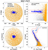 |
Fig. 1. Distribution of members (blue), candidates (orange), and non-members (grey) for NGC 2527 in sky position (top left), proper motion (bottom left), parallax (top right), and the CMD (bottom right). The blue line in the CMD constitutes the isochrone that corresponds to the age of NGC 2527 as provided by Cantat-Gaudin et al. (2020). The dashed red lines indicate a ‘zero-uncertainty boundary’, outside of which sources with negligible errors are not selected as candidates. Candidates that lay outside these boundaries therefore have significant uncertainties. |
The isochrones used for the CMD condition are obtained through the Padova web interface2, which computes the stellar evolutionary tracks with the PARSEC 1.2S and COLIBRI S37 models of Bressan et al. (2012), Chen et al. (2015), Pastorelli et al. (2020), and Marigo et al. (2017). To construct a compatible isochrone for each OC, we used cluster ages, distances, and extinctions reported by Cantat-Gaudin et al. (2020) and adopted solar metallicity. We correct the Gaia magnitudes of the isochrone points for the cluster distance and interstellar extinction. To calculate the extinction for the G and GRP passband, we use a precomputed extinction model provided by the dustapprox Python package (Fouesneau et al. 2022), which calculates the Gaia band extinction for a given extinction A0 at wavelength λ = 550 nm.
2.4. Maximum separation
As OCs are extended objects, the distribution of the members in the astrometric and photometric dimensions also depends on the morphology of the OC. To account for this feature in the candidate selection, we approximate the distribution in each dimension with a boundary, which we parameterise with a maximum separation Δ. The maximum separation Δ defines the maximum deviation from the cluster mean or isochrone that a source with zero uncertainties is allowed to have in order to be labelled as a candidate. In other words, it defines the boundary between candidates and non-members for sources with negligible uncertainties. This boundary is indicated by the red dashed line in Fig. 1.
For the proper motion, we use
 (6)
(6)
where σμα*, m and σμδ, m are the standard deviation of the OC members in each proper motion component, while σμα*, c and σμδ, c are the uncertainties of the weighted mean of the cluster proper motion components,
 (7)
(7)
where σμi, j is the error in the ith proper motion component of the jth member. For most OCs, the uncertainty in the cluster means is 10–100 times smaller than the standard deviation of the members, but for OCs with a small number of members which have relatively large errors, the uncertainty in the cluster means is significant.
For the parallax, we take into account the expected asymmetry in the parallax distribution; we do this primarily for nearby OCs, because of the inverse relation between parallax and distance. We therefore use a different value for Δϖ depending on whether the parallax of a source is greater or smaller than the cluster parallax,
 (8)
(8)
where
 (9)
(9)
The first term in Eq. (9) is the difference between the cluster parallax and the parallax of a hypothetical source that lies Rmax closer or farther away from the OC. We use
 (10)
(10)
where R90 is the smallest projected radius to enclose 90% of the members in sky position. The additional 15 pc serves the purpose of a lower boundary for small OCs, while also taking into account that the training members generally only constitute the core of the cluster. The second term in Eq. (9), parallel to the definition of Δμi, contains the uncertainty of the weighted mean parallax of the cluster. The third term contains an estimate of the uncertainty in the parallax zero-point ϖ0, where we use σϖ0 = 0.015 mas (Lindegren et al. 2021), which is significant for distant OCs. We offset the parallaxes in our cone search with zero points as a function of magnitude, colour, and ecliptic latitude according to the recipe provided by Lindegren et al. (2021).
Finally, for the colour and magnitude, we use
 (11)
(11)
and
 (12)
(12)
where we define ΔC, 90 and ΔG, 90 such that at least 90% of our training members would pass the isochrone candidate condition (Eq. (5)) when ΔC ≥ ΔC, 90 and ΔG ≥ ΔG, 90. We additionally use the constraint ΔG, 90/ΔC, 90 = 8 to obtain a single solution for each OC. This value approximately reflects the ratio between the ranges in colour and magnitude of sources in the CMD. By only letting 90% of the members pass the isochrone candidate condition, we generally prevent ΔC and ΔG from being skewed by training members that do not follow the isochrone, such as blue stragglers. In contrast, the constant values added in Eqs. (11) and (12) prevent the condition from being too restrictive. Their values effectively account for the effects of common phenomena such as binarity, stellar variability, and differential reddening, which cause individual cluster members to deviate from the isochrone. They also generally mitigate errors in the estimated age and assumed metallicity of the isochrone.
3. Method
In order to identify additional members of OCs, we make use of the Deep Sets (DS) neural network architecture developed by Zaheer et al. (2017). This architecture was designed to operate on sets, meaning unordered lists of objects, and therefore has the characteristic feature of returning the same output for every permutation of a given input. In our implementation of the DS architecture, we use this feature to perform the following classification task: given (i) a set of stars labelled as members of the same OC (support set) and (ii) an unlabelled candidate member for that OC, return a binary label, member or non-member, for the candidate. We train the neural network to determine when a candidate star is sufficiently similar to the member stars in the support set in order to be classified as a member. The OC members with p = 1.0 obtained by Cantat-Gaudin et al. (2020) constitute the member stars used for the support set. We use the same neural network architecture as Oladosu et al. (2020), who successfully applied the DS architecture to the analogous task of finding new members of stellar streams. These latter authors found that the DS architecture outperforms random forest baselines when trained and tested on synthetic data, that is, a synthetic stellar stream inserted in a real field of stars extracted from Gaia data, even when the random forest model is optimised for a subset of the members of the test stream in question. Compared to models that are trained on one specific stream, the DS architecture has the potential advantage of being able to learn higher-level member properties, which are shared among streams. Another advantage with respect to the random forest model is that there is no need for negative examples (non-members) when applying the model to a new stream. However, when applied to one of the few actual stellar streams with reliable members, the fine-tuned random forest model did better than the DS architecture trained on synthetic streams, although a DS architecture optimised for the real stream performed best. Oladosu et al. (2020) propose the difference in synthetic and real data as a possible explanation. In the case of OCs, thanks to recent contributions to OC membership lists (Cantat-Gaudin & Anders 2020), which include reliable membership lists for hundreds of OCs, we can avoid the use of synthetic examples. In addition, the members of an OC generally follow a positional and proper motion distribution that is, for the majority of OCs, approximately spherically symmetric, which is easier to learn than the elongated structure followed by the stars in a stellar stream. In parallax space in particular, in which sources have relatively large uncertainties, the roughly similar distances of OC members pose less of a challenge than the gradient in distances of a stellar stream.
We include diagrams of the model components in Appendix A. For a more detailed description of the neural network architecture, we refer to Zaheer et al. (2017).
3.1. Features
We attribute sources with a number of features on which the DS model has to base its membership predictions. For a feature to be effective, the (expected) distributions of members and non-members need to differ significantly in the feature space, as this enables the DS model to consistently differentiate the two classes. We use five source features, which relate to the sky position, proper motion, parallax, colour, and magnitude of a source, and three cluster features, namely mean parallax, age, and line-of-sight extinction, which are the same for each source associated with a given OC. For the age and line-of-sight extinction, we use the values reported by Cantat-Gaudin et al. (2020). Our calculations of the source features are described in the following sections.
3.1.1. Sky position separation
We use the projected radius fR between a source and the cluster centre,
 (13)
(13)
where D is the distance to the OC with respect to us and θ is the angular separation between the source and the cluster centre,
![Mathematical equation: $$ \begin{aligned} \theta = \cos ^{-1}\left[\sin (\delta )\sin (\delta _{c}) - \cos (\delta )\cos (\delta _{c})\cos (\alpha - \alpha _{c})\right], \end{aligned} $$](/articles/aa/full_html/2023/07/aa45952-23/aa45952-23-eq14.gif) (14)
(14)
with α and δ being the right ascension and declination of the source and αc and δc the right ascension and declination of the cluster centre.
3.1.2. Proper motion separation
We use a ‘proper motion separation’:
 (15)
(15)
which is a measure of the deviation of a a source from the mean proper motion of the OC.
3.1.3. Parallax separation
Similar to the proper motion feature, we have
 (16)
(16)
for a deviation measure in parallax space.
3.1.4. Isochrone vector
The fourth and fifth features are the two components of a vector that represents a source’s smallest separation from the isochrone:
where [Cic, Gic] is the point on the isochrone for which
 (17)
(17)
is minimised.
3.2. Training and validation sets
A training set and a validation set are created from the members and non-members associated with 243 OCs. These OCs meet the following criteria: they (i) have their age, distance, extinction, and at least 80 members with p = 1.0 available in the catalogue provided by Cantat-Gaudin et al. (2020), (ii) are not used to test the model (see Sect. 4), (iii) have a Galactic longitude that deviates by more than 60 degrees from the Galactic centre, and (iv) have a parallax of less than 4 mas. Conditions (iii) and (iv) are designed to exclude OCs with computationally expensive cone searches. The validation set, which includes 30% of these OCs, is used to monitor the performance of the model on unseen data during training. The remaining 70% are contained in the training set and the performance of the model on this set determines the optimisation of the model parameters during the training process. By training on the members and non-members of many different OCs, the model is able to learn the general distribution of OC members, making it capable of finding new members even for OCs it has not been trained on.
Instances of both sets are created as follows: each member and non-member is first attributed with a number of training features (see Sect. 3.1), which are designed to contain the relevant information of a source such that the model can make an accurate membership prediction. Next, we pair the member or non-member we want the model to classify with a support set consisting of a random set of members (excluding the source to be classified if it is also a member) of fixed size and from the same OC as the source to be classified. We then combine the source to be classified and the support set into a single tensor, which will be the input for the DS model. This tensor is created by concatenating the training features of the source to be classified with the training features of each member in the support set, resulting in a Ns × 2M matrix where Ns is the number of members in the support set and M is the number of training features per source. An instance of the training or validation set is then the pair of this input tensor and the binary label indicating whether the source to be classified is a member or non-member.
In order to augment the number of positive examples in our datasets, we create two instances with each member to be classified for the training or validation set, depending on which set the corresponding OC is in. Both instances will contain the same member to be classified, but a different random support set to prevent duplicity of the training and validation instances. From the set of non-members of each OC, we take five times the number of included members to be classified (i.e. ten times the number of unique members to classify) for that OC, which ensures a fixed ratio between members and non-members. The amount of non-members resulting from our candidate-selection process is generally much larger than the number of members for a given OC, and therefore in most cases all of the non-members to be classified in the training and validation set are unique. In the case where the number of non-members we want to include for a given OC is larger than the number of unique non-members for that OC, we pad the difference with randomly selected non-members of that OC.
3.3. Training process
To optimise the model parameters, we use the cross-entropy loss function
 (18)
(18)
where pij and qij are, respectively, the true probability and predicted probability of a source being classified as class i and class j (member or non-member). The true probability corresponds to the label of the source to be classified and is therefore either 0 or 1. In order to mitigate overfitting, we apply two types of regularisation during training. We use L2 regularisation, giving a total loss function
 (19)
(19)
where wi are the trainable parameters and γ determines the strength of the regularisation. In addition, we scale the gradients of the trainable parameters used in the optimisation process such that their norm does not exceed a certain value. We use PyTorch’s implementation of the ADAM optimiser (Kingma & Ba 2014) to minimise the loss function. To assess the performance of the model, we keep track of the F1-score, which is the harmonic mean of the recall and precision (see the caption of Fig. 2 for their definition). The F1-score is considered a suitable metric for data with a large class imbalance when the majority class is labelled as negative, which are the non-members in our case (Chicco & Jurman 2020). When the F1-score has not improved for 20 consecutive epochs, we stop the training process and use the model parameters that produced the maximum F1-score for the final model. Figure 2 shows the evolution of the loss and a number of metrics for the training and validation set.
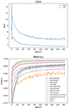 |
Fig. 2. Performance of the DS model during training. The top figure shows the evolution of the loss function (Eq. (19)) for the training and validation set. The bottom figure shows the evolution of a number of classification metrics based on the number of true positives TP, true negatives TN, false positives FP, and false negatives FN, including: precision |


3.4. Membership probability
We calculate a membership probability for each candidate member by applying the DS model on multiple samples of the candidate. For each sample, we recalculate the proper motion, parallax, magnitude, and colour of the candidate by sampling from a multi-variate normal distribution defined by the candidate’s uncertainties and the available correlations for these properties in the Gaia data. With the sampled properties, we calculate the new training feature values of the sample. We also supply a different random support set for each sample. The membership probability is then defined as the fraction of samples for which the DS model identifies the candidate as a member. We use a sample size of 100 to cover both the variance in the feature values and the support set members.
4. Results
The Python code and instructions for using the method are publicly available at the gaia_oc_amd repository on GitHub3. The generated membership lists are available at the CDS.
To demonstrate the effectiveness of our method, we tested the DS model on 167 OCs that (i) were provided with a membership list by Tarricq et al. (2022; hereafter T22), (ii) have their age, distance, extinction, and at least 20 members with p = 1.0 available in the catalogue provided by Cantat-Gaudin et al. (2020), (iii) are not in the training or validation set, and (iv) have a Galactic longitude that deviates by more than 30 degrees from the Galactic centre to lighten the computational load. We compare the members we obtain to the members obtained by T22. These latter authors used the Hierarchical Density-Based Spatial Clustering of Applications with Noise (HDBSCAN) clustering algorithm Campello et al. (2013) – which is considered a state-of-the-art method for determining OC members (Hunt & Reffert 2021) – to establish their membership lists. Tarricq et al. (2022) ran HDBSCAN on Gaia EDR3 parallax and proper motion dimensions (ϖ, μα*, μδ) and applied no additional selection criteria in sky position dimensions as they focused on studying the halos of OCs. We note that our method uses the same parallax and proper motion data as T22, but uses sky position and photometric data as well.
We also considered comparing with membership lists from Dias et al. (2021), as they assembled membership lists from various sources and a significant fraction of these also include G > 18 members. However, almost all their OCs with G > 18 members do not have a membership list available in Cantat-Gaudin et al. (2020). As such, a systematic comparison in which only members from Cantat-Gaudin et al. (2020) are used for the support set is not viable.
In Fig. 3, we present two Venn diagrams that show the overlap between the members from T22 and the members in this study. The top figure in Fig. 3 includes all members with a membership probability of p ≥ 0.1 and shows that we generally find the majority of the T22 members and also a significant number of additional members. In the most extreme cases, over 90% of the members we obtain for a single cluster are not in the corresponding T22 membership list. In the subsequent sections, we discuss the origins of the differences in the membership lists.
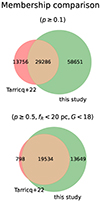 |
Fig. 3. Venn diagrams comparing the combined membership lists of the 167 test OCs from T22 and this study. The top figure compares the members with a membership probability of p ≥ 0.1, while the bottom figure compares the members with a membership probability of p ≥ 0.5, a projected radius of less than 20 pc, and a G-magnitude of brighter than 18. The members that only occur in T22 are labelled in red, those that only occur in this study are in green, and the overlapping members are labelled in orange. |
In Fig. 4, we compare the member distributions in sky position, proper motion, parallax, and the CMD of four OCs: NGC 2099, NGC 752, NGC 2682, and IC 4756. These plots serve as examples of the member distributions we obtain, and will be used as a reference to highlight some of the trends we observe when comparing the membership lists. They also show that the additional members fainter than G = 18 generally conform to the distribution of the T22 members in each dimension, which supports the credibility of their membership status.
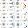 |
Fig. 4. Distributions of p ≥ 0.1 members of NGC 2099, NGC 752, NGC 2682, and IC 4756 found in this study (blue) and by T22 (orange) in (from left to right) sky position, parallax, proper motion, and CMD. |
4.1. Projected radius and G-magnitude
As our method and that used by T22 determine OC membership in a different way, the discrepancy between the membership lists is to be expected to some degree. However, many members are excluded from either list for trivial reasons. For example, in contrast to our candidates, T22 a priori excluded sources with G > 18 from their membership list. On the other hand, our method ascribes lower membership probabilities to sources with large projected radii, while the T22 membership probability does not depend on the sky position. If we analyse the members from T22 that we missed, that is, the members from T22 that we either select as non-members or ascribe a membership probability of p < 0.1, which together make up 32% of the total number of T22 members, we find that 73% of these were selected as candidates, but that the average projected radius of these candidates is 38.3 pc with a standard deviation of 3.1 pc. Sources beyond this radius are typically given very low membership probabilities as the training members from Cantat-Gaudin et al. (2020) usually do not extend far beyond the core of the cluster. A clear example of this can be seen in the sky position plot of NGC 2099 in Fig. 4, where the outskirts are only populated by T22 members. In order to show the significance of these differences, we present a similar comparison in the bottom plot of Fig. 3 where we only consider sources with G < 18 and with projected radii of less than 20 pc. As the high-probability sources are more relevant for comparison than the low-probability sources, we also consider only sources with a membership probability of p ≥ 0.5 for this plot. After these cuts, a total of 33 184 (38%) members in our study and 20 332 (47%) T22 members remain. This comparison shows that we find nearly all of the probable (p ≥ 0.5) T22 members within a 20 pc radius. For 61 OCs, we find 100% of these T22 members. We can also see that the fraction of new members is generally lower, as a large proportion of all p ≥ 0.1 members we obtain are G > 18 members, which are excluded from the bottom Venn diagram. The median fraction of p ≥ 0.1 members we obtain with G > 18 is 43.5%. For nearby OCs, which have more faint sources with high probabilities due to smaller astrometric uncertainties, the fraction of members we obtain with G > 18 and p ≥ 0.1 can be as large as 70%–80%.
4.2. Parallax, proper motion, and RUWE
The remaining differences between our results and those of T22 are primarily the result of the different treatments of the parallax and proper-motion dimensions between our study and theirs, which are data used by both methods. If we consider only the sources used for the bottom plot in Fig. 3, that is, sources with p ≥ 0.5, fr < 20 pc, and G < 18, we obtain median parallax and proper motion features  and
and  for our members, where the bounds indicate the 15th and 85th percentiles, while the same statistics for the selected T22 members are
  and
and  . Therefore, our method is, on average, effectively less ‘strict’ in the parallax and proper motion dimension. An aspect of our approach that could be relevant here is our inclusion of sources with a renormalised unit weight error (RUWE) of greater than 1.4, which are excluded in the T22 study. We find that, of our sources that have p ≥ 0.1, G < 18 and are not among the T22 members, 26% have a RUWE of above 1.4. However, the effect of these sources on the aforementioned distributions of fϖ and fμ is very small.
In contrast with the general trend of broader distributions in fϖ and fμ for our members, some OCs have T22 member distributions that are much more extended. For example, the OCs UPK 303, COIN-Gaia 30, ASCC 58, NGC 1901, and COIN-Gaia 13 have a much broader distribution of T22 members in proper motion compared to the training members, resulting in many of the T22 members being selected as non-members by our method. In Fig. 4, NGC 752 is another example of this. The statistics of all T22 members not selected as candidates also show the relative strictness of our proper motion condition. Of these missing T22 members, 67% failed to meet the proper motion condition. By comparison, only 27% failed to meet the parallax condition and only 20% failed to meet the isochrone condition. Clear examples of T22 members excluded by the parallax condition can be seen in the parallax plot of cluster IC 4756 in Fig. 4 and examples for T22 members excluded by the isochrone condition can be seen for the clusters NGC 2682 and NGC 2099.
5. Summary and conclusions
We developed a methodology to find new OC members in Gaia DR3 for the population of known OCs. This methodology is based on a deep neural network architecture, which is able to learn the distribution of highly reliable OC members in a high-dimensional space, meaning five-dimensional astrometry and photometry, and retrieve new members based on the similarities in these parameters. To train our method, we take advantage of the high-quality OC catalogue built using Gaia DR2 (Cantat-Gaudin et al. 2020) and EDR3 (Castro-Ginard et al. 2022), which contains around 2500 OCs with membership lists, mean astrometric parameters, and astrophysical information.
The method presented here is available as an open-source Python tool at the gaia_oc_amd repository on GitHub. This python package has built-in functions to go through all the steps described in the previous sections, from querying OC members and their mean parameters, generating the different cone searches in the Gaia archive and creating the member, non-member, and candidates datasets, to training the model and using it to find new OC members. Documentation and a step-by-step tutorial in the form of a Python notebook are included within the package. The generated membership lists are also made available through the CDS.
When comparing our results with independent membership determinations for a subset of the OC catalogue (Tarricq et al. 2022), we are able to retrieve 100% of their members within 20 pc of the cluster centre while adding some new members at bright magnitudes (G ≤ 18). More importantly, we are able to extend membership lists to fainter magnitudes – down to the Gaia magnitude limit – in a homogeneous way for the first time on the whole OC catalogue. The distribution of the members we obtain in this magnitude domain conforms to that of the members from Tarricq et al. (2022) in both the astrometric and photometric dimensions, which provides good evidence for their reliability. Extending the membership list beyond G = 18 is needed for forthcoming spectroscopic surveys such as WEAVE and 4MOST, whose input target lists are based entirely on Gaia, and in their low-resolution modes, they can observe sources fainter than G = 18 mag. These surveys will complement Gaia with radial velocities for stars with GRVS ∼ 16 and chemical abundances for all the observed stars. In the context of the present work, this will allow us to further refine OC membership lists and retrain our method for a more accurate membership determination.
Having more complete membership lists for the OCs also enables further scientific applications. So far, Gaia has redefined the OC census, providing a better characterisation of their astrometric properties, the addition of hundreds of new objects to the catalogue, and the estimation of some astrophysical properties that only depend on the shape of the OC isochrone in the CMD. However, further improvements to the OC catalogue, such as the estimation of masses or the dynamical evolution of OCs (and their members) through the Galactic disc, rely on a complete description of the OC in the whole Gaia magnitude range and the distribution of its member stars in the CMD, also accounting for possible selection effects on these stars (Cantat-Gaudin et al. 2023).
Available at https://github.com/MGJvanGroeningen/gaia_oc_amd
In the original model from Zaheer et al. (2017), this block is repeated only three times. This is the only difference compared to the version from Oladosu et al. (2020) and thus compared to our model as well.
Acknowledgments
This work has made use of results from the European Space Agency (ESA) space mission Gaia, the data from which were processed by the Gaia Data Processing and Analysis Consortium (DPAC). Funding for the DPAC has been provided by national institutions, in particular, the institutions participating in the Gaia Multilateral Agreement. The Gaia mission website is http://www.cosmos.esa.int/gaia. The authors are current or past members of the ESA Gaia mission team and of the Gaia DPAC. This research has made use of the tool provided by Gaia DPAC (https://www.cosmos.esa.int/web/gaia/dr3-software-tools) to reproduce (E)DR3 Gaia photometric uncertainties described in the GAIA-C5-TN-UB-JMC-031 technical note using data in Riello et al. (2021). This work was (partially) funded by the Spanish MICIN/AEI/10.13039/501100011033 and by “ERDF A way of making Europe” by the “European Union” through grants RTI2018-095076-B-C21 and PID2021-122842OB-C21, and the Institute of Cosmos Sciences University of Barcelona (ICCUB, Unidad de Excelencia ‘María de Maeztu’) through grant CEX2019-000918-M.
References
- Balbinot, E., Santiago, B. X., da Costa, L. N., Makler, M., & Maia, M. A. G. 2011, MNRAS, 416, 393 [NASA ADS] [Google Scholar]
- Bressan, A., Marigo, P., Girardi, L., et al. 2012, MNRAS, 427, 127 [NASA ADS] [CrossRef] [Google Scholar]
- Campello, R. J. G. B., Moulavi, D., & Sander, J. 2013, Adv. Knowl. Discovery Data Min., 7819, 160 [Google Scholar]
- Cantat-Gaudin, T., & Anders, F. 2020, A&A, 633, A99 [NASA ADS] [CrossRef] [EDP Sciences] [Google Scholar]
- Cantat-Gaudin, T., Jordi, C., Vallenari, A., et al. 2018, A&A, 618, A93 [NASA ADS] [CrossRef] [EDP Sciences] [Google Scholar]
- Cantat-Gaudin, T., Anders, F., Castro-Ginard, A., et al. 2020, A&A, 640, A1 [NASA ADS] [CrossRef] [EDP Sciences] [Google Scholar]
- Cantat-Gaudin, T., Fouesneau, M., Rix, H.-W., et al. 2023, A&A, 669, A55 [NASA ADS] [CrossRef] [EDP Sciences] [Google Scholar]
- Castro-Ginard, A., Jordi, C., Luri, X., et al. 2018, A&A, 618, A59 [NASA ADS] [CrossRef] [EDP Sciences] [Google Scholar]
- Castro-Ginard, A., Jordi, C., Luri, X., Cantat-Gaudin, T., & Balaguer-Núñez, L. 2019, A&A, 627, A35 [NASA ADS] [CrossRef] [EDP Sciences] [Google Scholar]
- Castro-Ginard, A., Jordi, C., Luri, X., et al. 2020, A&A, 635, A45 [NASA ADS] [CrossRef] [EDP Sciences] [Google Scholar]
- Castro-Ginard, A., McMillan, P. J., Luri, X., et al. 2021, A&A, 652, A162 [NASA ADS] [CrossRef] [EDP Sciences] [Google Scholar]
- Castro-Ginard, A., Jordi, C., Luri, X., et al. 2022, A&A, 661, A118 [NASA ADS] [CrossRef] [EDP Sciences] [Google Scholar]
- Chen, Y., Bressan, A., Girardi, L., et al. 2015, MNRAS, 452, 1068 [Google Scholar]
- Chicco, D., & Jurman, G. 2020, BMC Genomics, 21, 1 [CrossRef] [Google Scholar]
- Clevert, D. A., Unterthiner, T., & Hochreiter, S. 2015, ArXiv e-prints [arXiv:1511.07289] [Google Scholar]
- Dalton, G., Trager, S. C., Abrams, D. C., et al. 2012, SPIE Conf. Ser., 8446, 84460P [Google Scholar]
- de Jong, R. S., Bellido-Tirado, O., Chiappini, C., et al. 2012, SPIE Conf. Ser., 8446, 84460T [Google Scholar]
- Dias, W. S., Alessi, B. S., Moitinho, A., & Lépine, J. R. D. 2002, A&A, 389, 871 [NASA ADS] [CrossRef] [EDP Sciences] [Google Scholar]
- Dias, W. S., Monteiro, H., Moitinho, A., et al. 2021, MNRAS, 504, 356 [NASA ADS] [CrossRef] [Google Scholar]
- Ferreira, F. A., Corradi, W. J. B., Maia, F. F. S., Angelo, M. S., & Santos, J. F. C. 2020, MNRAS, 496, 2021 [NASA ADS] [CrossRef] [Google Scholar]
- Fouesneau, M., Andrae, R., Sordo, R., & Dharmawardena, T. 2022, https://github.com/mfouesneau/dustapprox [Google Scholar]
- Gaia Collaboration (Prusti, T., et al.) 2016, A&A, 595, A1 [NASA ADS] [CrossRef] [EDP Sciences] [Google Scholar]
- Gaia Collaboration (Brown, A. G. A., et al.) 2018, A&A, 616, A1 [NASA ADS] [CrossRef] [EDP Sciences] [Google Scholar]
- Gaia Collaboration (Brown, A. G. A., et al.) 2021, A&A, 649, A1 [NASA ADS] [CrossRef] [EDP Sciences] [Google Scholar]
- Gaia Collaboration (Vallenari, A., et al.) 2023, A&A, 674, A1 [NASA ADS] [CrossRef] [EDP Sciences] [Google Scholar]
- Hinton, G. E., Srivastava, N., Krizhevsky, A., Sutskever, I., & Salakhutdinov, R. R. 2012, ArXiv e-prints [arXiv:1207.0580] [Google Scholar]
- Hunt, E. L., & Reffert, S. 2021, A&A, 646, A104 [NASA ADS] [CrossRef] [EDP Sciences] [Google Scholar]
- Kharchenko, N. V., Piskunov, A. E., Schilbach, E., Röser, S., & Scholz, R. D. 2013, A&A, 558, A53 [NASA ADS] [CrossRef] [EDP Sciences] [Google Scholar]
- Kingma, D. P., & Ba, J. 2014, ArXiv e-prints [arXiv:1412.6980] [Google Scholar]
- Krone-Martins, A., & Moitinho, A. 2014, A&A, 561, A57 [NASA ADS] [CrossRef] [EDP Sciences] [Google Scholar]
- Lindegren, L., Bastian, U., Biermann, M., et al. 2021, A&A, 649, A4 [EDP Sciences] [Google Scholar]
- Liu, L., & Pang, X. 2019, ApJS, 245, 32 [NASA ADS] [CrossRef] [Google Scholar]
- Malhan, K., & Ibata, R. A. 2018, MNRAS, 477, 4063 [Google Scholar]
- Marigo, P., Girardi, L., Bressan, A., et al. 2017, ApJ, 835, 77 [Google Scholar]
- Mateu, C., Read, J. I., & Kawata, D. 2018, MNRAS, 474, 4112 [Google Scholar]
- Meingast, S., Alves, J., & Rottensteiner, A. 2021, A&A, 645, A84 [NASA ADS] [CrossRef] [EDP Sciences] [Google Scholar]
- Monteiro, H., Barros, D. A., Dias, W. S., & Lépine, J. R. D. 2021, Front. Astron. Space Sci., 8, 62 [NASA ADS] [CrossRef] [Google Scholar]
- Oladosu, A., Xu, T., Ekfeldt, P., et al. 2020, ArXiv e-prints [arXiv:2007.04459] [Google Scholar]
- Pastorelli, G., Marigo, P., Girardi, L., et al. 2020, MNRAS, 498, 3283 [Google Scholar]
- Riello, M., De Angeli, F., Evans, D. W., et al. 2021, A&A, 649, A3 [NASA ADS] [CrossRef] [EDP Sciences] [Google Scholar]
- Sim, G., Lee, S. H., Ann, H. B., & Kim, S. 2019, J. Korean Astron. Soc., 52, 145 [NASA ADS] [Google Scholar]
- Tarricq, Y., Soubiran, C., Casamiquela, L., et al. 2021, A&A, 647, A19 [NASA ADS] [CrossRef] [EDP Sciences] [Google Scholar]
- Tarricq, Y., Soubiran, C., Casamiquela, L., et al. 2022, A&A, 659, A59 [NASA ADS] [CrossRef] [EDP Sciences] [Google Scholar]
- Zaheer, M., Kottur, S., Ravanbakhsh, S., et al. 2017, Adv. Neural Inf. Process. Syst., 30 [Google Scholar]
Appendix A: Model architecture
A diagram of the complete DS model is given in Fig. A.2. The first part of the model consists of a permutation equivariant layer (PEL) and an exponential linear unit (ELU) (Clevert et al. 2015) activation function, which is repeated five4 times.
In the PEL, expanded into its components in Fig. A.1, the input follows two parallel tracks. In Fig. A.1, the track on the left contains one linear layer, which performs the operation
 (A.1)
(A.1)
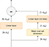 |
Fig. A.1. Diagram containing the operations in the PEL. The variables in parentheses indicate the dimensions of the tensors between operations. The batch dimension is left out for clarity. In the linear layer on the right track, the biases are set to zero. |
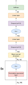 |
Fig. A.2. Diagram of the complete DS model. Details of the PEL are given in Fig. A.1. The variables and values in the brackets indicate the dimensions of the tensors between operations and the batch dimension is left out for clarity. The symbol Ns refers to the size of the support set, M to the number of training features, and dh to the hidden dimension of the network. |
on its input vector x, with dimensionality din, and returns a new vector x′, with dimensionality dout. The weight matrix Wn and bias vector bn of linear layer n constitute trainable parameters of the model, which are to be optimised during the training process. In the right track, the mean over the set dimension is taken first, followed by another linear layer. Finally, the output from the right track is subtracted from the output of the left track. We note that, as the input to the first PEL consists of the training features, the mean features of the support set members are part of the result from the first ‘mean over set dimension’. The membership prediction is therefore partly based on the mean features of the members in the support set. The term ‘permutation equivariant’ refers to the feature of the PEL whereby a permutation (of the set dimension) of the input gives the same result as the same permutation on the output, that is,
 (A.2)
(A.2)
After the PEL blocks, taking the mean over the set dimension guarantees the invariance of the output with respect to a permutation of the model input, fulfilling the precondition for a model operating on sets. This is followed by a dropout layer, which randomly sets elements of the input tensor to zero during training, with a 50% probability for each element. This prevents over-reliance on certain features of the input, which helps prevent overfitting to the training data (Hinton et al. 2012). The final linear layer transforms its input, which is a vector with a hidden dimension dh, to a 2D vector, corresponding to the two classes: member and non-member. The softmax layer then converts values in the 2D vector to values that sum to 1 and can thus be interpreted as a probability for each class. Finally, the class with the highest probability is attributed to the candidate member included in the model input.
All Figures
|
Fig. 1. Distribution of members (blue), candidates (orange), and non-members (grey) for NGC 2527 in sky position (top left), proper motion (bottom left), parallax (top right), and the CMD (bottom right). The blue line in the CMD constitutes the isochrone that corresponds to the age of NGC 2527 as provided by Cantat-Gaudin et al. (2020). The dashed red lines indicate a ‘zero-uncertainty boundary’, outside of which sources with negligible errors are not selected as candidates. Candidates that lay outside these boundaries therefore have significant uncertainties. |
| In the text | |
|
Fig. 2. Performance of the DS model during training. The top figure shows the evolution of the loss function (Eq. (19)) for the training and validation set. The bottom figure shows the evolution of a number of classification metrics based on the number of true positives TP, true negatives TN, false positives FP, and false negatives FN, including: precision |
| In the text | |
|
Fig. 3. Venn diagrams comparing the combined membership lists of the 167 test OCs from T22 and this study. The top figure compares the members with a membership probability of p ≥ 0.1, while the bottom figure compares the members with a membership probability of p ≥ 0.5, a projected radius of less than 20 pc, and a G-magnitude of brighter than 18. The members that only occur in T22 are labelled in red, those that only occur in this study are in green, and the overlapping members are labelled in orange. |
| In the text | |
|
Fig. 4. Distributions of p ≥ 0.1 members of NGC 2099, NGC 752, NGC 2682, and IC 4756 found in this study (blue) and by T22 (orange) in (from left to right) sky position, parallax, proper motion, and CMD. |
| In the text | |
|
Fig. A.1. Diagram containing the operations in the PEL. The variables in parentheses indicate the dimensions of the tensors between operations. The batch dimension is left out for clarity. In the linear layer on the right track, the biases are set to zero. |
| In the text | |
|
Fig. A.2. Diagram of the complete DS model. Details of the PEL are given in Fig. A.1. The variables and values in the brackets indicate the dimensions of the tensors between operations and the batch dimension is left out for clarity. The symbol Ns refers to the size of the support set, M to the number of training features, and dh to the hidden dimension of the network. |
| In the text | |
Current usage metrics show cumulative count of Article Views (full-text article views including HTML views, PDF and ePub downloads, according to the available data) and Abstracts Views on Vision4Press platform.
Data correspond to usage on the plateform after 2015. The current usage metrics is available 48-96 hours after online publication and is updated daily on week days.
Initial download of the metrics may take a while.