| Issue |
A&A
Volume 675, July 2023
|
|
|---|---|---|
| Article Number | A196 | |
| Number of page(s) | 12 | |
| Section | Catalogs and data | |
| DOI | https://doi.org/10.1051/0004-6361/202345951 | |
| Published online | 24 July 2023 | |
The Trans-Heliospheric Survey
Radial trends in plasma parameters across the heliosphere★
1
Department of Physics & Astronomy, University of Delaware,
104 The Green, 217 Sharp Lab,
Newark, DE
19716, USA
e-mail: bmaruca@udel.edu
2
Bartol Research Institute,
104 The Green, 217 Sharp Lab,
Newark, DE
19716, USA
3
Center for Space Physics, Boston University,
725 Commonwealth Ave, Room 506,
Boston, MA
02215, USA
4
Space Science and Engineering, Southwest Research Institute,
6220 Culebra Road,
San Antonio, TX
78238, USA
5
Department of Mechanical Engineering,
44 Cummington Mall,
Boston University, 44 Cummington Mall,
Boston, MA
02215, USA
6
NASA Headquarters Science Mission Directorate,
300 Hidden Figures Way SW,
Washington, DC
20546, USA
7
Mullard Space Science Laboratory, University College London,
Holmbury House, Holmbury St. Mary,
Dorking
RH5 6NT, UK
8
Department of Astrophysical Sciences, Princeton University,
Peyton Hall, 4 Ivy Lane,
Princeton, NJ
08544, USA
9
Heliophysics Science Division, NASA Goddard Space Flight Center,
8800 Greenbelt Rd,
Greenbelt, MD
20771, USA
10
Laboratory for Atmospheric and Space Physics,
1234 Innovation Drive,
Boulder, CO
80303, USA
11
School of Chemical and Physical Sciences, Victoria University of Wellington,
Gate 7, Kelburn Parade, Kelburn,
Wellington
6012, New Zealand
12
University of Maryland Baltimore County,
1000 Hilltop Circle,
Baltimore, MD
21250, USA
Received:
19
January
2023
Accepted:
6
April
2023
Context. Though the solar wind is characterized by spatial and temporal variability across a wide range of scales, long-term averages of in situ measurements have revealed clear radial trends: changes in average values of basic plasma parameters (e.g., density, temperature, and speed) and a magnetic field with a distance from the Sun.
Aims. To establish our current understanding of the solar wind's average expansion through the heliosphere, data from multiple spacecraft needed to be combined and standardized into a single dataset.
Methods. In this study, data from twelve heliospheric and planetary spacecraft - Parker Solar Probe (PSP), Helios 1 and 2, Mariner 2 and 10, Ulysses, Cassini, Pioneer 10 and 11, New Horizons, and Voyager 1 and 2 - were compiled into a dataset spanning over three orders of magnitude in heliocentric distance. To avoid introducing artifacts into this composite dataset, special attention was given to the solar cycle, spacecraft heliocentric elevation, and instrument calibration.
Results. The radial trend in each parameter was found to be generally well described by a power-law fit, though up to two break points were identified in each fit.
Conclusions. These radial trends are publicly released here to benefit research groups in the validation of global heliospheric simulations and in the development of new deep-space missions such as Interstellar Probe.
Key words: Sun: heliosphere / solar wind / Sun: corona
Data associated with Figs. 1–7 (full Table 2) are only available at the CDS via anonymous ftp to cdsarc.cds.unistra.fr (130.79.128.5) or via https://cdsarc.cds.unistra.fr/viz-bin/cat/J/A+A/675/A196
© The Authors 2023
 Open Access article, published by EDP Sciences, under the terms of the Creative Commons Attribution License (https://creativecommons.org/licenses/by/4.0), which permits unrestricted use, distribution, and reproduction in any medium, provided the original work is properly cited.
This article is published in open access under the Subscribe to Open model. Subscribe to A&A to support open access publication.
1 Introduction
The solar wind's expansion through interplanetary space is driven and affected by the complex interaction of many different plasma processes acting across a wide range of spatial and temporal scales (Marsch 2006; Verscharen et al. 2019). Though the solar wind exhibits strong variability, observations of "radial trends" – long-term average values in plasma parameters and the magnetic field as functions of distance, r, from the Sun – have proven an important means for characterizing the solar wind's typical expansion. For example, the radial trend in proton (ionized hydrogen) temperature has been consistently observed (citations below) to fall off more slowly than predicted by adiabatic expansion, which indicates substantial solar-wind heating well outside of the corona.
Previous studies of radial trends in particle and magnetic-field parameters have utilized in situ observations from the Parker Solar Probe (PSP), Helios, Ulysses, Wind, ACE, Cluster, and MESSENGER spacecraft individually and in combination (e.g., Marsch et al. 1982a,b; Bavassano et al. 2001, 2000; Maksimovic et al. 2005; Bruno & Carbone 2005, 2013; Matteini et al. 2007; Štverák et al. 2008, 2009, 2015; Hellinger et al. 2011, 2013; Telloni et al. 2015; McComas et al. 2017; Zank et al. 2018; Elliott et al. 2019; Parashar et al. 2019; Perrone et al. 2019a,b; Chhiber et al. 2021; Adhikari et al. 2022; Cuesta et al. 2022a,b; Shi et al. 2022). Some related studies have exploited Ulysses' unique orbit to also explore variations with solar latitude (e.g., McComas et al. 2000, 2003; Verscharen et al. 2021).
This study, the Trans-Heliospheric Survey, sought the widest possible coverage. Data from twelve heliospheric and planetary spacecraft - PSP, Helios 1 and 2, Mariner 2 and 10, Ulysses, Cassini, Pioneer 10 and 11, New Horizons, and Voyager 1 and 2 – were compiled into a dataset spanning over six decades and over three orders of magnitude in r. The resultant radial trends extend from the outer corona to the termination shock. The compilation and analysis of this dataset is presented in Sect. 2. Section 3 describes the results of this analysis and provides a case study of how these radial trends can be utilized in designing of future deep-space missions. Section 4 offers final remarks, including a look at ongoing work to extend this study.
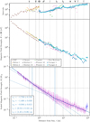 |
Fig. 1 Multi-spacecraft radial trend analysis (plots versus distance, r, from the Sun) of magnetic field strength, B = |B|. Vertical lines indicate the semi-major axes of the orbits of the eight planets (black) and three dwarf planets (gray): Ceres, Pluto, and Eris. The top plot shows the number of one-hour intervals (Sect. 2) for which each spacecraft measured B. The middle plot shows each spacecraft's median B value for each r bin with at least 25 measurements. The bottom plot shows the trend in the scaled magnetic field strength, B/⟨B⟩⊕. Circular markers indicate median values, and vertical lines indicate the 25th- to 75th-percentile ranges (thick) and the 10th- to 90th-percentile ranges (thin). Bins at r > 80 au have blue markers to indicate that they are outliers due to the effects of the termination shock. The best-fit curve (Eq. (8)) is plotted in solid cyan; dashed cyan lines indicate the break points, and dotted cyan lines extend each power-law segment beyond its specified domain. |
2 Data analysis
The radial analysis of the seven solar-wind parameters are shown in Figs. 1 to 7. Figure 1 shows the magnetic-field strength (B ≡ |B|). Figures 2, 3, and 4 show the proton number-density (np), bulk speed1 (vp ≡ |vp|), and scalar temperature (Tp), respectively. Figures 5 and 6 show the (proton) Alfvén speed,
 (1)
(1)

Figure 7 shows the proton scalar beta,
 (3)
(3)
All of these parameters are plotted with respect to distance, r, from the Sun. This section details the methodology (data selection, binning, and fitting) used to generate these figures, and Sect. 3 presents the interpretation of them.
This study's primary observations were taken from publicly available archives for twelve heliospheric missions whose trajectories spanned particularly wide r ranges (Table 1). Though most of these archives already had a one-hour cadence, data in the remaining archives were averaged down to match.
As this study focused on radial trends in quasi-ecliptic solar wind, some data were removed from the datasets prior to analysis. Ulysses data were restricted to those before the spacecraft's Jovian encounter (1992 February 18; Neugebauer et al. 1996) to avoid the portions of its trajectory at extreme heliographic latitudes. Likewise, to minimize data from beyond the termination shock, data from r > 100 au were excised. This criterion only applied to Voyager 1 and 2, and (as shown below) did retain some data affected by the termination shock, though the affected data were excised from any fits.
The one-hour data from each mission's dataset were sorted among logarithmically uniform r bins: 80 bins from r = 0.06 to 100 au.
The top plots in Figs. 1 to 7 differ among each other for two reasons. First, not all parameters have values available from all spacecraft. For example, Fig. 1 shows no data from New Horizons since it does not carry a magnetometer. Second, even for a given spacecraft, not all parameters have values available at the same times. For example, some of PSP's one-hour intervals have magnetic-field measurements but no ion measurements.
Each of the middle plots in Figs. 1 to 7 reveals a clear, steady radial trend for its corresponding parameter. Though data from the various missions are remarkably consistent with each other, some significant offsets are apparent. For example, PSP returned systematically lower values for B (Fig. 1) and lower for vp (Fig. 3) than either Helios 1 or 2 even at the same r values. Though this could indicate a calibration error, a more likely cause is solar-cycle variation. The PSP observations in this study are primarily from near solar minimum. In contrast, the Helios 1 and 2 datasets span a larger fraction of the solar cycle.
To partially correct for systematic variations with the solar cycle, a method similar to that of Smith et al. (2001a) was implemented. Each one-hour datum for each parameter from each spacecraft was "scaled" by a pseudo-contemporaneous (i.e., adjusted for propagation time), average value at r = 1 au using the OMNI dataset in the following manner. For example, a parameter k is measured to have a value k0 at a time t0, when the spacecraft is at a radial distance r0 and measures the solar wind's speed to be vp0. Assuming that the velocity of a given parcel of solar-wind plasma is approximately constant (Fig. 3), radial, and highly supersonic, the plasma observed at r = r0 was or will be at r = 1 au at a time
 (4)
(4)
For a given k measurement, ⟨k⟩⊕ denotes the average OMNI value of k over a 27-day interval centered on t⊕. This averaging partially accounts for differences in heliographic latitude between Earth and the observing spacecraft. Thus, the ratio
 (5)
(5)
indicates the scaled measurement of k − a quantification of how the k value measured at r = r0 compares to typical, pseudo-contemporaneous values at r = 1 au.
The bottom plots in Figs. 1 to 7 show the trend in each scaled parameter,  , with r. In contrast to the top and middle plots, these are "composite" plots in that they incorporate one-hour intervals from all spacecraft as a single dataset.
The data shown in the bottom plots in Figs. 1 to 7 have also been provided in supplementary data files included with this publication: one file for each parameter. Table 2 shows a portion of the data in the magnetic-field file to aid potential users in parsing the data files. All numeric values in the data file have three significant figures, though some measured values have less precision than this. For example, some datasets only give r to two decimal places, which constitutes only two significant figures for r values between 0.1 and 1 au. Also, the r values do not perfectly align across these files since the radial coverage varies somewhat among the parameters. Each r value is the median r value for the measurements of the corresponding parameter in the corresponding r bin.
The scaling method used to generate the bottom plots in Figs. 1 to 7 removes any sense of absolute scale from the data: the scaled version,  , of any parameter, k, is dimensionless (Eq. (5)) and has a median value of ≈1 at r = 1 au. Nevertheless, this method does preserve the overall radial trends (i.e., how the parameters vary with r), and effectively corrects for much of the long-term variation in parameter values with the solar cycle. For example, without scaling, the aforementioned discrepancy between PSP and Helios observations seen in the middle plots would produce a "kink" at r ≈ 0.3 au (the approximate perihelion of both Helios spacecraft) in the composite radial trends in the bottom plots. With scaling, though, the bottom plots show little or no indication of such defects.
Radial trends in solar-wind parameters have often effectively (e.g., Bavassano et al. 2000, 2001; Maksimovic et al. 2005; Štverák et al. 2009, 2015; Hellinger et al. 2011) been modeled with simple power laws in r:
 (6)
(6)
where the normalization factor, C, and the index, α1, are free parameters. This study's unprecedented radial coverage - almost three orders of magnitude in r – reveals that the radial trends in most solar-wind parameters are more complex. Nevertheless, to provide continuity with prior studies, power-law fits were still used but one or more "break points" were introduced as free parameters. A singly broken power law has a single break point at r = ra, where the index changes from α1 to α2:
 (7)
(7)
A doubly broken power law has two break points at r = ra and rb, which separate regions with indices α1, α2, and α3:
 (8)
(8)
These models remain continuous (though not differentiable) at each break point.
The scaled, composite radial trends shown in the bottom plots of Figs. 1 to 7 were each fit with a singly or doubly broken power law. For each fit, each datum was weighted by the inverse square root of the number of one-hour intervals in its corresponding r bin. The data at r > 80 au, which were heavily affected by the termination shock (e.g., Stone et al. 2005), were excluded from the fits. The best-fit values (and uncertainties therein) for the break point(s) and the indices are provided in the plots and in Table 3.
Because the data in each of the bottom plots were scaled to conditions at r = 1 au (Eq. (5)), the units of each fit are entirely arbitrary. For any parameter, k, to convert its scaled fit,  , to one in physical units, kfit(r), one only needs to utilize the median k value at a reference point such as r = 1 au:
 (9)
(9)
For convenience, Table 4 provides median parameters' values at r = 1 au from the OMNI dataset spanning Solar Cycles 20 – 24 (from 1964 October 01 to 2019 December 31).
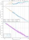 |
Fig. 2 Multi-spacecraft radial trend analysis of proton number density, np. This figure follows the same format as Fig. 1. |
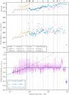 |
Fig. 3 Multi-spacecraft radial trend analysis of proton bulk speed, vp = |vp|. This figure follows the same format as Fig. 1. |
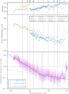 |
Fig. 4 Multi-spacecraft radial trend analysis of proton temperature, Tp. This figure follows the same format as Fig. 1. |
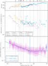 |
Fig. 5 Multi-spacecraft radial trend analysis of (proton) Alfvén speed, |

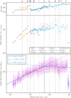 |
Fig. 6 Multi-spacecraft radial trend analysis of Alfvén number, NA = vp/vA. This figure follows the same format as Figure 1. |
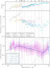 |
Fig. 7 Multi-spacecraft radial trend analysis of proton beta, ßp = 2μ0kBnpTp/B2. This figure follows the same format as Fig. 1. |
3 Results
3.1 Radial trends
The radial trend (Fig. 1, bottom plot) in magnetic field strength, B, is well fit by a doubly broken power law. Though B(r) monotonically decreases until the termination shock, the rate of its falloff decreases with increasing r. This is at least qualitatively consistent with the model of Parker (1958, 1963), which predicts that B(r) is approximately proportional to r−2 near the Sun and r−1 far from it (Burlaga 1995).
For both proton density, np, and speed, vp, each radial trend (Figs. 2 and 3, bottom plots) is well fit by a power law with a single, relatively "soft" break (i.e., small change from α1 to α2). The radial trend in np exhibits a rapid falloff with r. An unbroken power-law fit of np(r), (not shown in Fig. 2) returned a power-law index of α = −2.017 ± 0.022, though that fit's substantial residuals (at r < 0.7 au and r > 10 au) warranted the addition of a single break. In contrast, vp(r) exhibits little variation in the outer heliosphere (until the termination shock) and actually slowly increases with r until about the orbit of Venus, which suggests that appreciable solar-wind acceleration continues well beyond the corona. The best-fit break points in np(r) and vp(r) are of roughly the same magnitude, though they are not mutually consistent to within the fit uncertainties. The sum of the np and vp indices before the breaks (α1 values) and the sum of the indices after the breaks (α2 values) are both very close to −2. A radial trend of npvp ∝ r−2 would be consistent with a radial, steady-state flow in which particles are conserved.
The radial trends (Figs. 4, 5, and 6, bottom plots) in proton temperature (Tp), Alfvén speed (vA), and Alfvén number (NA) are all well fit by singly broken power laws. Though adding a second break to each fit was attempted, the relatively high scatter of the data (compared, e.g., to the radial trend in B) meant that it produced only modest improvement in the alignment of the fit curve with the data. Curiously, the fits of the radial trends in B, Tp, vA, and NA all produced a break point around r ≈ 4.5 to 5.0 au. The fact that the trend in B should share a break point with those in υA and NA is not entirely surprising since υA and NA depend strongly on B. In contrast, B and Tp are measured with entirely separate instruments, which suggests that their common break point is the result of some phenomenon in the solar wind. Prior studies (e.g., Williams et al. 1995; Smith et al. 2001b; Zank et al. 2018; Hollick et al. 2018; Sokół et al. 2019; Zirnstein et al. 2022) have identified pickup ions as a substantial energy source for the outer heliosphere's solar wind – driving turbulent fluctuations that ultimately heat the plasma. Though this may be coincidental, this break point's location roughly coincides with Jupiter's orbit, and all of the outer heliospheric missions in this study included a Jovian encounter in their trajectories. Jupiter's magnetosphere includes a tail that extends to at least Saturn's orbit (Russell 1993), so it could impact the radial evolution of a substantial portion of the outer heliosphere's solar wind.
Proton beta, βp, exhibits the least well-defined radial trend (Fig. 7) of the parameters considered in this study. The range of typical βp values at a given r value is comparable to the range seen across all r values in this study. The trend was fit by a doubly broken power law with positive indices in the very inner and outer heliosphere and a negative one between. One limitation, though, to the utility of the radial trend in βp is that in the outer heliosphere (r ≳ 20 au), pickup ions provide the dominant source of internal pressure (McComas et al. 2017; Zank et al. 2018), which significantly complicates a fluid analysis of the solar wind. Nevertheless, even in this regime, βp remains an important parameter for various kinetic phenomena.
The radial trends exhibit a curious anomaly from r ≈ 45 to 60 au. It manifests most prominently as a decrease in np and an increase in vp, though a slight increase in Tp is also apparent. Notably, the trend in B shows no such deviation. The cause of this feature in the radial trends remains unclear. It seems to originate in the Voyager 2 dataset (see the middle plot of Fig. 2 in particular), but a visual inspection of the data revealed no obvious insights. If this is the result of some transient structure in the outer heliosphere, it must have been remarkably large and persistent since the spacecraft spent years traversing this range of r values.
Datasets used in this study.
Extract of supplementary data file: percentiles of scaled magnetic-field strength, B/⟨B⟩⊕, versus heliocentric distance, r.
Median solar-wind parameters at r = 1 au (OMNI, Solar Cycles 20 – 24).
3.2 Case study: instrument design
The radial trends produced in this study offer a useful tool in the development of new deep-space heliophysics missions. To enhance reliability and reduce development costs, new missions often fly with instruments closely based on those from prior missions, but adjustments are often required to account for differences in the plasma environment encountered by each spacecraft. For example, plasma instruments on PSP (Fox et al. 2016; Kasper et al. 2016) drew substantial heritage from those on Wind (Acuña et al. 1995; Ogilvie et al. 1995; Lin et al. 1995) but were optimized to measure plasma that is hotter and denser than in near-Earth solar wind.
As a simple example of this design process, one can consider a typical electrostatic analyzer (ESA), which uses detectors to count the number of particles collected in a set sample period (Verscharen et al. 2019). Each detector targets a narrow range of particle velocities centered on a velocity u. Under typical conditions, the number of particles of a species j collected is approximately (Verscharen et al. 2019, Eq. (75))
 (10)
(10)
where mj is the mass of a j particle, fj is the velocity distribution function (VDF) of j particles, and G is ESA's "geometric factor," which accounts for the instrument's resolution and collecting area.
As an example, one can consider the task of modifying an ESA designed for measuring solar-wind protons (j = p) at r = 1 au to instead measure them at r = 40 au. An appropriate adjustment would be to alter G so that the proton count, ΔNp, remains roughly the same when the ESA targets protons moving at the proton's bulk velocity (i.e., u = vp). If the protons have a Maxwellian VDF, then
 (11)
(11)
Thus, the optimal geometric factor would scale as
 (12)
(12)
Based on the fits of the radial trends summarized in Figs. 2 to 4,
 (13)
(13)

which indicates that a proton ESA at r = 40 au would need a geometric factor about 66 times as large as one at r = 1 au.
A change in an ESA's geometric factor can be achieved in various ways (Verscharen et al. 2019, Eq. (76)). Though G is proportional to the collecting area, A, of the instrument, increasing A by a factor of 66 would produce an unpractically large instrument. Alternatively, G is also proportional to the sample time, Δt, so the geometric factor could be increased by reducing ESA's cadence. Typically, Δt is chosen based on a relevant timescale such as the cyclotron period, which for a particle species j, is
 (15)
(15)
where qj is the charge of a j particle. From the radial trend in Fig. 1,
 (16)
(16)

By sheer coincidence, this is almost the exact adjustment required for the geometric factor. Thus, increasing Δt by a factor of about 65 would increase G by the desired amount with little deleterious effect on the instrument's ability to observe phenomena whose timescales are tied to the cyclotron period.
The preceding analysis is admittedly a simplistic one. A more realistic design process would explicitly account for the instrument's noise and not focus on a single particle velocity but instead consider the instrument's response to the full VDF − especially in the context of the mission's specific science objectives. For example, given the lower proton temperatures at 40 versus 1 au, a higher-energy resolution may be needed, which would also affect the geometric factor. Nevertheless, this analysis does demonstrate the utility of radial trends for such efforts.
4 Conclusion
This work, the Trans-Heliospheric Survey, constitutes one of the most comprehensive analyses to date of in situ solar-wind observations: data from twelve spacecraft (Table 1) spanning three orders of magnitude in distance from the Sun. The resulting radial trends (Figs. 1 to 7) elucidate the "big picture" of solarwind expansion. Though this study utilized large-scale spacial and temporal averaging, the complexities of the radial trends that it produced can only ever be fully understood as the aggregate effect of the various multiscale processes at work in the solar wind (Verscharen et al. 2019). In this regard, this study has made strides in the long journey toward characterizing the solar wind's complex dynamics.
The radial trends in the study are also published here as a service to the heliophysics community. As demonstrated in Sect. 3.2, they can be a very useful tool in planning future deep-space missions such as Interstellar Probe (Brandt et al. 2022, 2023). Additionally, many groups (e.g., Opher et al. 2015; Chhiber et al. 2019a,b; Kleimann et al. 2022) who have been developing global simulations of the heliosphere may find these radial trends helpful in the validation their work. Though the radial evolution of any given run of a simulation may depart significantly from the trends presented herein, the average behavior of a large ensemble of simulations should be much more consistent (e.g., Chhiber et al. 2021).
The success of this study motivates further exploration of large-scale variations in the solar wind. Indeed, this present work should be regarded as Version 1 of the Trans-Heliospheric Survey since work has already begun on Version 2, which will incorporate several enhancements. First, Version 2 will utilize expanded datasets from PSP and New Horizons as well as a new dataset from Solar Orbiter. Second, this new version may include radial trends in additional parameters (e.g., vector components of the magnetic field and proton velocity). Third and most importantly, Version 2 will include "joint trends" that quantify how solar-wind parameters vary with both distance from the Sun and heliographic latitude (i.e., angle out of the Sun's equatorial plane). This effort presents some challenges because of the limited data coverage (especially at extreme latitudes). Nevertheless, the trajectories of the present study's twelve spacecraft (Table 1) do provide significant coverage out to at least modest latitudes, which will be augmented with data from the Solar Orbiter mission.
This study exclusively utilized publicly available datasets, which did limit it to relatively low-cadence time series of the most fundamental plasma parameters. Access to data from more detailed analyses of particle measurements would enable studies of how departures from local thermodynamic equilibrium (e.g., temperature anisotropy, relative drifts, and beams) change as the solar wind expands. Likewise, higher-cadence data (even for the fundamental parameters) would enable trends in wave and turbulence activities to be produced. Though some studies of these types have already been completed (e.g., Matteini et al. 2007; Parashar et al. 2019; Chhiber et al. 2021; Cuesta et al. 2022a,b), much more work is required to better understand the interplay between the solar wind's large-scale expansion and its microkinetic phenomena.
Another limitation of this study is that its source datasets combined observations from all types of solar wind. There is no reason to expect that the radial evolution of solar wind emerging from different types of the source regions should be similar. Nevertheless, reliably categorizing solar-wind observations can be very challenging (Verscharen et al. 2019, Sect. 1.3 and references therein). Variations in charge states and elemental composition have been associated with differences in coronal magnetic structure, but many of these spacecraft used in this study had no instruments capable of such measurements. The simplest and most traditional means for distinguishing a source region is solar-wind speed, υp, but even this presents a problem. The strong overlap between "slow" and "fast" solar wind means no clear cutoff value for υp exists. Even if such a value did exist, Fig. 3 indicates that it would vary significantly with r in the inner heliosphere.
Acknowledgements
B.A.M., R.A.Q., B.L.A., and B.M.W. acknowledge support from NASA Grant 80NSSC22K0645. B.L.A. is also supported by NASA Grants 80NSSC22K1011 and 80NSSC20K1844. B.A.M. and W.H.M. are supported by the Delaware Space Observation Center (DSpOC), which is funded by NASA Grant 80NSSC22K0884. W.H.M. is also partially supported by NASA under a Heliophysics GI Program Grant 80NSSC21K1765 and by the IMAP project through Princeton Subcontract SUB0000317 to the University of Delaware. D.V. is supported by STFC Ernest Rutherford Fellowship ST/P003826/1 and STFC Consolidated Grants ST/S000240/1 and ST/W001004/1. R.B. is supported by NASA Grants 80NSSC21K1767, 80NSSC21K1458 and 80NSSC21K0739. R.C. acknowledges support from NASA Grants 80NSSC18K1210 and 80NSSC18K1648. The authors extend their sincere thanks to the spacecraft/instrument teams whose data were used in this study and the teams behind the OMNI dataset, OMNIWeb, COHOWeb, and CDAWeb. B.A.M. thanks Parisa S. Mostafavi, Michael V. Paul, Justyna M. Sokol, and Lynn B. Wilson, III for useful discussions and the anonymous reviewer for several helpful suggestions. B.A.M. and D.V. benefited from discussion at the International Space Science Institute (ISSI) in Bern, through ISSI International Team project #563, which is led by Leon Ofman and Lan K. Jian. The preparation of this manuscript made use of the SAO/NASA Astrophysics Data System (ADS).
References
- Acuña, M. H., Ogilvie, K. W., Baker, D. N., et al. 1995, Space Sci. Rev., 71, 5 [Google Scholar]
- Adhikari, L., Zank, G. P., Zhao, L. L., & Telloni, D. 2022, ApJ, 933, 56 [NASA ADS] [CrossRef] [Google Scholar]
- Bavassano, B., Pietropaolo, E., & Bruno, R. 2000, J. Geophys. Res., 105, 15959 [NASA ADS] [CrossRef] [Google Scholar]
- Bavassano, B., Pietropaolo, E., & Bruno, R. 2001, J. Geophys. Res., 106, 10659 [NASA ADS] [CrossRef] [Google Scholar]
- Brandt, P. C., Provornikova, E. A., Cocoros, A., et al. 2022, Acta Astronautica, 199, 364 [NASA ADS] [CrossRef] [Google Scholar]
- Brandt, P. C., Provornikova, E., Bale, S. D., et al. 2023, Space Sci. Rev., 219, 18 [NASA ADS] [CrossRef] [Google Scholar]
- Bruno, R., & Carbone, V. 2005, Living Rev. Solar Phys., 2, 4 [NASA ADS] [CrossRef] [Google Scholar]
- Bruno, R., & Carbone, V. 2013, Living Rev. Solar Phys., 10, 2 [NASA ADS] [CrossRef] [Google Scholar]
- Burlaga, L. F. 1995, Interplanetary Magnetohydrodynamics (New York, NY: Oxford University Press) [Google Scholar]
- Chhiber, R., Usmanov, A. V., Matthaeus, W. H., & Goldstein, M. L. 2019a, ApJS, 241, 11 [Google Scholar]
- Chhiber, R., Usmanov, A. V., Matthaeus, W. H., & Goldstein, M. L. 2019b, ApJS, 242, 12 [NASA ADS] [CrossRef] [Google Scholar]
- Chhiber, R., Usmanov, A. V., Matthaeus, W. H., & Goldstein, M. L. 2021, ApJ, 923, 89 [NASA ADS] [CrossRef] [Google Scholar]
- Cuesta, M. E., Chhiber, R., Roy, S., et al. 2022a, ApJ, 932, L11 [NASA ADS] [CrossRef] [Google Scholar]
- Cuesta, M. E., Parashar, T. N., Chhiber, R., & Matthaeus, W. H. 2022b, ApJS, 259, 23 [NASA ADS] [CrossRef] [Google Scholar]
- Elliott, H. A., McComas, D. J., Zirnstein, E. J., et al. 2019, ApJ, 885, 156 [Google Scholar]
- Fox, N. J., Velli, M. C., Bale, S. D., et al. 2016, Space Sci. Rev., 204, 7 [Google Scholar]
- Hellinger, P., Matteini, L., Štverák, Š., Trávníček, P. M., & Marsch, E. 2011, J. Geophys. Res. (Space Phys.), 116, 9105 [NASA ADS] [CrossRef] [Google Scholar]
- Hellinger, P., Trávníček, P. M., Štverák, v., Matteini, L., & Velli, M. 2013, J. Geophys. Res. (Space Phys.), 118, 1351 [NASA ADS] [CrossRef] [Google Scholar]
- Hollick, S. J., Smith, C. W., Pine, Z. B., et al. 2018, ApJ, 863, 76 [NASA ADS] [CrossRef] [Google Scholar]
- Kasper, J. C., Abiad, R., Austin, G., et al. 2016, Space Sci. Rev., 204, 131 [Google Scholar]
- Kleimann, J., Dialynas, K., Fraternale, F., et al. 2022, Space Sci. Rev., 218, 1 [NASA ADS] [CrossRef] [Google Scholar]
- Lin, R. P., Anderson, K. A., Ashford, S., et al. 1995, Space Sci. Rev., 71, 125 [CrossRef] [Google Scholar]
- Maksimovic, M., Zouganelis, I., Chaufray, J.-Y., et al. 2005, J. Geophys. Res., 110, A09104 [NASA ADS] [Google Scholar]
- Marsch, E. 2006, Living Rev. Solar Phys., 3, 1 [NASA ADS] [CrossRef] [Google Scholar]
- Marsch, E., Rosenbauer, H., Schwenn, R., Mühlhäuser, K.-H., & Neubauer, F. M. 1982a, J. Geophys. Res., 87, 35 [NASA ADS] [CrossRef] [Google Scholar]
- Marsch, E., Schwenn, R., Rosenbauer, H., et al. 1982b, J. Geophys. Res., 87, 52 [Google Scholar]
- Matteini, L., Landi, S., Hellinger, P., et al. 2007, Geophys. Res. Lett., 34, 20105 [NASA ADS] [CrossRef] [Google Scholar]
- McComas, D. J., Barraclough, B. L., Funsten, H. O., et al. 2000, J. Geophys. Res. (Space Phys.), 105, 10419 [NASA ADS] [CrossRef] [Google Scholar]
- McComas, D. J., Elliott, H. A., Schwadron, N. A., et al. 2003, Geophys. Res. Lett., 30, 1517 [Google Scholar]
- McComas, D. J., Zirnstein, E. J., Bzowski, M., et al. 2017, ApJS, 233, 8 [NASA ADS] [CrossRef] [Google Scholar]
- Neugebauer, M., Goldstein, B. E., Smith, E. J., & Feldman, W. C. 1996, J. Geophys. Res., 101, 17047 [NASA ADS] [CrossRef] [Google Scholar]
- Ogilvie, K. W., Chornay, D. J., Fritzenreiter, R. J., et al. 1995, Space Sci. Rev., 71, 55 [Google Scholar]
- Opher, M., Drake, J., Zieger, B., & Gombosi, T. 2015, ApJ, 800, L28 [NASA ADS] [CrossRef] [Google Scholar]
- Parashar, T. N., Cuesta, M., & Matthaeus, W. H. 2019, ApJ, 884, L57 Parker, E. N. 1958, ApJ, 128, 664 [Google Scholar]
- Parker, E. N. 1963, Interplanetary Dynamical Processes (New York, NY: John Wiley & Sons) [Google Scholar]
- Perrone, D., Stansby, D., Horbury, T. S., & Matteini, L. 2019a, MNRAS, 483, 3730 [Google Scholar]
- Perrone, D., Stansby, D., Horbury, T. S., & Matteini, L. 2019b, MNRAS, 488, 2380 [Google Scholar]
- Russell, C. T. 1993, Rep. Progr. Phys., 56, 67 [Google Scholar]
- Shi, C., Velli, M., Bale, S. D., et al. 2022, Phys. Plasmas, 29, 122901 [Google Scholar]
- Smith, C. W., Matthaeus, W. H., Zank, G. P., et al. 2001a, J. Geophys. Res., 106, 8253 [Google Scholar]
- Smith, C. W., Matthaeus, W. H., Zank, G. P., et al. 2001b, J. Geophys. Res. (Space Phys.), 106, 8253 [NASA ADS] [CrossRef] [Google Scholar]
- Sokół, J. M., Kubiak, M. A., & Bzowski, M. 2019, ApJ, 879, 24 [CrossRef] [Google Scholar]
- Stone, E. C., Cummings, A. C., McDonald, F. B., et al. 2005, Science, 309, 2017 [NASA ADS] [CrossRef] [Google Scholar]
- Štverák, S., Trávníček, P., Maksimovic, M., et al. 2008, J. Geophys. Res. (Space Phys.), 113, A03103 [Google Scholar]
- Štverák, V., Maksimovic, M., Trávníček, P. M., et al. 2009, J. Geophys. Res. (Space Phys.), 114, A05104 [Google Scholar]
- Štverák, V., Trávníček, P. M., & Hellinger, P. 2015, J. Geophys. Res. (Space Phys.), 120, 8177 [CrossRef] [Google Scholar]
- Telloni, D., Bruno, R., & Trenchi, L. 2015, ApJ, 805, 46 [NASA ADS] [CrossRef] [Google Scholar]
- Verscharen, D., Klein, K. G., & Maruca, B. A. 2019, Living Rev. Solar Phys., 16, 5 [NASA ADS] [CrossRef] [Google Scholar]
- Verscharen, D., Bale, S. D., & Velli, M. 2021, MNRAS, 506, 4993 [NASA ADS] [CrossRef] [Google Scholar]
- Williams, L. L., Zank, G. P., & Matthaeus, W. H. 1995, J. Geophys. Res. (Space Phys.), 100, 17059 [NASA ADS] [CrossRef] [Google Scholar]
- Zank, G. P., Adhikari, L., Zhao, L.-L., et al. 2018, ApJ, 869, 23 [NASA ADS] [CrossRef] [Google Scholar]
- Zirnstein, E. J., Möbius, E., Zhang, M., et al. 2022, Space Sci. Rev., 218, 28 [NASA ADS] [CrossRef] [Google Scholar]

All Tables
Extract of supplementary data file: percentiles of scaled magnetic-field strength, B/⟨B⟩⊕, versus heliocentric distance, r.
All Figures
|
Fig. 1 Multi-spacecraft radial trend analysis (plots versus distance, r, from the Sun) of magnetic field strength, B = |B|. Vertical lines indicate the semi-major axes of the orbits of the eight planets (black) and three dwarf planets (gray): Ceres, Pluto, and Eris. The top plot shows the number of one-hour intervals (Sect. 2) for which each spacecraft measured B. The middle plot shows each spacecraft's median B value for each r bin with at least 25 measurements. The bottom plot shows the trend in the scaled magnetic field strength, B/⟨B⟩⊕. Circular markers indicate median values, and vertical lines indicate the 25th- to 75th-percentile ranges (thick) and the 10th- to 90th-percentile ranges (thin). Bins at r > 80 au have blue markers to indicate that they are outliers due to the effects of the termination shock. The best-fit curve (Eq. (8)) is plotted in solid cyan; dashed cyan lines indicate the break points, and dotted cyan lines extend each power-law segment beyond its specified domain. |
| In the text | |
|
Fig. 2 Multi-spacecraft radial trend analysis of proton number density, np. This figure follows the same format as Fig. 1. |
| In the text | |
|
Fig. 3 Multi-spacecraft radial trend analysis of proton bulk speed, vp = |vp|. This figure follows the same format as Fig. 1. |
| In the text | |
|
Fig. 4 Multi-spacecraft radial trend analysis of proton temperature, Tp. This figure follows the same format as Fig. 1. |
| In the text | |
|
Fig. 5 Multi-spacecraft radial trend analysis of (proton) Alfvén speed, |
| In the text | |
|
Fig. 6 Multi-spacecraft radial trend analysis of Alfvén number, NA = vp/vA. This figure follows the same format as Figure 1. |
| In the text | |
|
Fig. 7 Multi-spacecraft radial trend analysis of proton beta, ßp = 2μ0kBnpTp/B2. This figure follows the same format as Fig. 1. |
| In the text | |
Current usage metrics show cumulative count of Article Views (full-text article views including HTML views, PDF and ePub downloads, according to the available data) and Abstracts Views on Vision4Press platform.
Data correspond to usage on the plateform after 2015. The current usage metrics is available 48-96 hours after online publication and is updated daily on week days.
Initial download of the metrics may take a while.