| Issue |
A&A
Volume 675, July 2023
|
|
|---|---|---|
| Article Number | A162 | |
| Number of page(s) | 20 | |
| Section | The Sun and the Heliosphere | |
| DOI | https://doi.org/10.1051/0004-6361/202141816 | |
| Published online | 14 July 2023 | |
Precision electron measurements in the solar wind at 1 au from NASA’s Wind spacecraft⋆
1
Space Sciences Laboratory, University of California, Berkeley, CA 94720, USA
2
Physics Department, University of California, Berkeley, CA 94720, USA
3
Mullard Space Science Laboratory, University College London, Dorking RH5 6NT, UK
4
Space Science Center, University of New Hampshire, Durham, NH 03824, USA
Received:
16
July
2021
Accepted:
14
September
2021
Abstract
Context. The non-equilibrium characteristics of electron velocity distribution functions (eVDFs) in the solar wind are key to understanding the overall plasma thermodynamics as well as the origin of the solar wind. More generally, they are important in understanding heat conduction and energy transport in all weakly collisional plasmas. Solar wind electrons are not in local thermodynamic equilibrium, and their multicomponent eVDFs develop various non-thermal characteristics, such as velocity drifts in the proton frame and temperature anisotropies as well as suprathermal tails and heat fluxes along the local magnetic field direction.
Aims. This work aims to characterize precisely and systematically the nonthermal characteristics of the eVDF in the solar wind at 1 au using data from the Wind spacecraft.
Methods. We present a comprehensive statistical analysis of solar wind electrons at 1 au using the electron analyzers of the 3D-Plasma instrument on board Wind. This work uses a sophisticated algorithm developed to analyze and characterize separately the three populations – core, halo and strahl – of the eVDF up to super-halo energies (2 keV). This algorithm calibrates these electron measurements with independent electron parameters obtained from the quasi-thermal noise around the electron plasma frequency measured by Wind’s Thermal Noise Receiver (TNR). The code determines the respective set of total electron, core, halo, and strahl parameters through non-linear least-square fits to the measured eVDF, properly taking into account spacecraft charging and other instrumental effects, such as the incomplete sampling of the eVDF by particle detectors.
Results. We use four years, approximately 280 000 independent measurements, of core, halo, and strahl electron parameters to investigate the statistical properties of these different populations in the slow and fast solar wind. We discuss the distributions of their respective densities, drift velocities, temperature, and temperature anisotropies as functions of solar wind speed. We also show distributions with solar wind speed of the total density, temperature, temperature anisotropy, and heat flux of the total eVDF, as well as those of the proton temperature, proton-to-electron temperature ratio, proton-β and electron-β. Intercorrelations between some of these parameters are also discussed.
Conclusions. The present data set represents the largest, high-precision collection of electron measurements in the pristine solar wind at 1 au. It provides a new wealth of information on electron microphysics. Its large volume will enable future statistical studies of parameter combinations and their dependences under different plasma conditions.
Key words: solar wind / plasmas / methods: data analysis
A copy of the dataset is available as yearly files at NASA SPDF via https://doi.org/10.48322/rgf7-3h67 (Salem & Pulupa 2023)
e-mail: This email address is being protected from spambots. You need JavaScript enabled to view it.
© ESO 2023
1. Introduction
The contribution of electrons to the generation, acceleration, and evolution of the solar wind is still a critical and unsolved problem in solar wind physics (Marsch 2006; Verscharen et al. 2019b). For the development of predictive, physics-based solar wind models, a more accurate understanding of electron physics is crucial (Scudder 2019b).
Electrons are the most abundant particle species in all fully ionized plasmas, such as the solar wind. Despite their negligible contribution to the total solar wind momentum flux, they have a significant impact on the overall dynamics and thermodynamics of the solar wind for multiple reasons: (1) their high mobility adjusts quasi-neutrality on very short timescales compared to any other plasma timescales (Feldman et al. 1975); (2) their pressure gradient creates a significant electric field, which can lead to ambipolar diffusion and electrostatic acceleration (Lemaire & Scherer 1971, 1973; Scudder 1992, 1994, 1996; Scudder 2019a; Maksimovic et al. 1997, 2001; Zouganelis et al. 2004, 2005; Pierrard 2012); and (3) the observed nonzero skewness of the electron velocity distribution function (eVDF) provides the solar wind with a significant heat flux (e.g., Feldman et al. 1976; Scime et al. 1994a, 1999, 2001; Salem et al. 2003b; Bale et al. 2013; Halekas et al. 2020, 2021).
The kinetic properties of the electrons are fully described by the eVDF. Indeed, solar wind eVDFs have a complex structure that evolves with heliocentric distance. This evolution is the result of a delicate balance between several competing processes involving the Sun’s gravitation, the magnetic field, the electric field, Coulomb collisions and wave–particle interactions (with background electromagnetic turbulence and/or via plasma micro-instabilities; Verscharen et al. 2019b). This balance is restated by the generalized Ohm’s law (GOL), a steady-state electron equation of motion in the ion frame of reference (Rossi & Olbert 1970; Scudder 2019a,c). Information on these various processes is embedded in the eVDFs, with direct implications for electron heat conduction, as well as for the energy budget and the physics of the expanding solar wind (Hollweg 1974, 1976; Cranmer 2009; Štverák et al. 2015; Scudder 2019a).
Observations show that the solar wind eVDF at 1 au consists of three main components (Feldman et al. 1975; Rosenbauer et al. 1977; Pilipp et al. 1987a,b; Hammond et al. 1996; Lin 1998; Fitzenreiter et al. 1998; Maksimovic et al. 2000, 2005b; Gosling et al. 2001; Salem et al. 2003b, 2007; Štverák et al. 2009; Halekas et al. 2020): a primary cool thermal core (∼10 eV, ∼95% relative density), a superthermal halo (∼50 eV, ∼4% relative density), and a field-aligned anti-Sunward beam called strahl (∼100 − 1000 eV, ∼1% relative density). This core-halo-strahl structure is illustrated in Fig. 1. The top row shows a 2D view of the eVDFs of these three components in the ion frame, projected in a plane parallel and perpendicular to the local magnetic field [v∥, v⊥]. The bottom row highlights each component in a parallel cut through their eVDFs. The core is well described by a bi-Maxwellian distribution, while the halo population is well described by a (bi-)κ-distribution with large velocity tails in the eVDF (Feldman et al. 1975; Maksimovic et al. 2005b; Štverák et al. 2009; Wilson 2019a,b). The strahl has a more complicated cone-shaped structure, with an angular width that is highly variable between slow and fast solar wind, evolves with distance from the Sun, and depends on energy (Pilipp et al. 1987a,b; Hammond et al. 1996; Ogilvie et al. 1999; Anderson et al. 2012; Gurgiolo & Goldstein 2016; Graham et al. 2017; Horaites et al. 2018b; Berčič et al. 2019, 2020; Halekas et al. 2020).
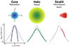 |
Fig. 1. Illustration of the three solar wind electron populations: the core, halo, and strahl. The top row shows a 2D view of the eVDFs of these three components, and the bottom row highlights each component in parallel cuts through the eVDFs. |
Each population often exhibits temperature anisotropies and rather large relative drifts parallel or antiparallel to the local magnetic field with respect to the other populations and the solar wind ions (Feldman et al. 1975; Štverák et al. 2008; Pulupa et al. 2014a). The three populations and their temperature anisotropies are more distinctive in the fast solar wind. This observation is usually attributed to collisional effects, which are stronger in the slow solar wind (Salem et al. 2003b; Marsch 2006). Although the individual drift speeds of the core, halo, and strahl relative to the ions globally satisfy quasi-neutrality and the zero-current condition, they correspond to a substantial heat flux, usually directed anti-Sunward. On a larger scale, studies of the radial evolution of eVDFs show that the relative density of the halo increases radially, while that of the strahl decreases at heliocentric distances greater than 0.3 au (Maksimovic et al. 2005b; Štverák et al. 2009; Halekas et al. 2020). At the same time, the angular width of the strahl increases with distance (Hammond et al. 1996; Graham et al. 2017; Berčič et al. 2019, 2020). These results suggest that the halo electrons are strahl electrons that have been backscattered and pitch-angle diffused by mechanisms that remain unidentified.
Both collisional and collisionless processes have been suggested as being responsible for controlling these electron nonthermal properties, via Coulomb collisions (Scudder & Olbert 1979a,b; Phillips & Gosling 1990; Lie-Svendsen et al. 1997; Landi & Pantellini 2003; Salem et al. 2003b; Štverák et al. 2008; Bale et al. 2013; Landi et al. 2012, 2014; Horaites et al. 2015, 2019; Boldyrev & Horaites 2019; Berčič et al. 2021) and/or (resonant or nonresonant) wave–particle interactions (Gary et al. 1975, 1994, 1999; Gary 1993; Krafft & Volokitin 2003; Vocks et al. 2005; Gary & Saito 2007; Shevchenko & Galinsky 2010; Seough et al. 2015; Kajdič et al. 2016; Horaites et al. 2018a; Roberg-Clark et al. 2018a,b, 2019; Verscharen et al. 2019a; Vasko et al. 2019; Jeong et al. 2020; Micera et al. 2020; Jagarlamudi et al. 2021; Innocenti et al. 2020; Cattell et al. 2021), respectively. On the other hand, a more recent theoretical paradigm (Scudder 2019a) predicts that the nonthermal shape of the eVDFs is a corollary of the strong parallel electric field needed to enforce the GOL balance so that no currents flow in the plasma, in a variant of Dreicer’s transient runaway process (Dreicer 1959, 1960; Fuchs et al. 1986).
At energies above those of the halo and strahl, the eVDF at times exhibits a super-halo (Lin 1980; Wang et al. 2012, 2015), a fourth population with energies from about 2 to 200 keV. The super-halo seems to be a quasi-isotropic and steady-state feature of the solar wind, although its origin still remains unknown (Yang et al. 2015).
To date, our understanding of the processes that regulate the solar wind electron properties and how the electrons couple to the ions are not fully understood (e.g., Marsch 2006; Verscharen et al. 2019b). This work aims to accurately and systematically characterize and quantify the nonthermal features of solar wind eVDFs and extract the properties of their core, halo, and strahl components using data from NASA’s Wind spacecraft (s/c; Acuña et al. 1995; Harten & Clark 1995). Wind is best suited for this study, with its well-designed, high resolution, particle and field instrumentation, the 3D Plasma (Lin et al. 1995) and the WAVES (Bougeret et al. 1995) experiments, respectively, and over 26 years of continuous data collection (i.e., over 2.5 solar cycles worth of data) to allow statistically significant studies of the variation and evolution of the solar wind electron properties. This is key to shedding light on the underlying physical processes at play to control the nonthermal eVDF shapes and properties, and ultimately solve the electron physics puzzle in the solar wind and in electron astrophysics in general (Verscharen et al. 2022).
Precision measurements of electrons are crucial for understanding the thermodynamics and microphysics of the plasma. These measurements are difficult to make and interpret: the low mass of electrons renders them especially susceptible to s/c charging effects in addition to inherent limitations in instrument capabilities. Indeed, the eVDF in the vicinity of the s/c is severely polluted at low energies (a few eV) by photo-electrons and secondary electrons emitted by the s/c body, and distorted by the electric field created by s/c charging. This electric field modifies both the energy and the direction of motion incident solar wind electrons (Grard 1973; Garrett 1981; Whipple 1981; Goertz 1989; Scime et al. 1994b; Pulupa et al. 2014a). Photo-electrons and secondary electrons contribute artificial counts to measured electron spectra at energies lower or equal to the energy associated with the s/c electric potential ϕ. Correcting for these effects is a difficult task since ϕ varies with the electron properties (density, temperature, etc.) that one wishes to measure. These corrections are complicated by the fact that the eVDF is measured within a finite energy range [Emin, Emax] (Song et al. 1997; Salem et al. 2001; Génot & Schwartz 2004). For typical electron detectors in the solar wind, Emin ∼ 5–10 eV, usually above the varying eϕ, so a variable part of the electron core is missing (Salem et al. 2001).
There are various ways of addressing these issues, the most natural being proper instrumentation measuring the s/c electric potential itself. Direct onboard measurements of the s/c potential using DC electric field instruments (Cully et al. 2007) have only been implemented on missions such as Cluster, THEMIS, MMS, Parker Solar Probe and Solar Orbiter. Older space missions such as Helios, Wind, or Ulysses do not have such DC electric field measurements and analyzing their electron data requires very careful handling and assessment of s/c charging and other instrumental effects.
Salem et al. (2001) discuss the various ways to tackle these effects in the absence of direct s/c potential measurements and propose an alternative, robust, technique to calibrate data from the electrostatic analyzers. These methods use data from ultra-sensitive radio receivers that measure the ubiquitous quasi-thermal noise (QTN) around the electron plasma frequency. From the plasma QTN, one can unambiguously derive the total electron density (Meyer-Vernet & Perche 1989; Issautier et al. 1998; Meyer-Vernet et al. 1998, 2017; Salem et al. 2001) as a reference.
In this paper, we introduce an automated analysis method that corrects for the s/c potential using thermal-noise measurements from Wind’s electric-field antennas, based on the Salem et al. (2001)’s technique. We then fit the three component structure of the corrected electron spectra to analytical expressions for the eVDFs. Applying our method to 4 years of Wind data, we present a large statistical survey of 280 000 reliable eVDF parameters in the solar wind at 1 au. This method and the resulting data set will be important cornerstones for future studies of specific electron processes in the solar wind.
In Sect. 2, we describe the instrumentation and the data products that we use in this work. In Sect. 3, we present the different stages of the eVDF analysis technique. In Sect. 4, we present the results of our fit analysis, showing first the statistics of the total electron parameters, such as total density, temperature, temperature anisotropy and heat flux of the total eVDF, as functions of the solar wind speed. Section 4 also presents the statistical distributions of the three electron components – core, halo and strahl – separately, and intercorrelations between core, halo and strahl properties are also shown and discussed. Section 5 presents a discussion of our results on electron properties at 1 au. Finally, Sect. 6 presents a conclusion synthesizing the new results from this work.
2. Wind instrumentation and data sets
To perform the present work, we use electron and wave data, as well as solar wind plasma moments and magnetic field vectors from various instruments on the Wind s/c. Here we describe these instruments and associated data products.
Wind was launched in November 1994. With its complete package of high resolution wave and particle instruments and extended intervals near or at the Lagrange point L1, it has been an ideal and unique platform providing continuously high time resolution – wave and particle – data ever in the solar wind at 1 au. Wind has now provided more than two solar cycles worth of data, allowing for comprehensive studies of waves, wave–particle coupling and of the microphysics of the solar wind in general (Wilson et al. 2021). We consider data from free solar wind intervals (see next section) only, so the data presented here concerns the physics of the pristine, unperturbed solar wind.
We use full 3D electron distribution functions from the Electron ElectroStatic Analyzers (EESA), part of the 3D-Plasma (3DP) experiment (Lin et al. 1995). We also use plasma wave spectra around the electron plasma frequency from the Thermal Noise Receiver (TNR), part of the WAVES experiment (Bougeret et al. 1995). These are used for the QTN spectroscopy technique (described below) to determine electron parameters independently of the 3DP spectra in order to calibrate the 3DP electron data and estimate the s/c floating potential (Salem et al. 2001).
In addition, we use solar wind plasma moments, namely solar wind speed and proton temperature, from the 3DP ion analyzers (Lin et al. 1995) and the SWE Faraday Cup (Ogilvie et al. 1995), as well as spin-resolution (3 s) magnetic field data from the Magnetic Field Investigation (MFI; Lepping et al. 1995).
2.1. The EESA electrostatic analyzers
The pair of EESAs make 3D measurements of eVDFs from 3 eV to 30 keV with a high time resolution, high sensitivity, wide dynamic range and a good energy and angular resolution. The EESA-Low (EESA-L) analyzer covers the range of 3 eV to 1.1 keV, with a smaller geometric factor than the EESA-High (EESA-H) analyzer, which covers the energy range 300 eV to 30 keV. Both instruments have operational fields of view of 180° and 15 logarithmically spaced energy channels. They sweep out 4π steradians in one s/c spin (spin period of 3 s). The data are combined on board into 88 angular bins for both instruments. Because of the available telemetry rate, the full 3D eVDFs are transmitted only every ∼96 s when Wind is at L1, but onboard computed moments (calculated from the EESA-L distributions, up to the 3rd order) are transmitted with a cadence of 3 s.
The s/c charging effects generally combine with other instrumental effects, such as the incomplete sampling of the VDFs due to a nonzero low-energy threshold of the energy sweeping in the electron spectrometer (Song et al. 1997; Salem et al. 2001). Consequently, all the moments of the eVDFs are affected as well (Salem et al. 2001, and references therein). A careful analysis of solar wind eVDFs requires therefore a full correction of these effects.
2.2. The Thermal Noise Receiver
The TNR is a very sensitive digital spectrum analyzer designed to measure the electron QTN around the electron plasma frequency. The QTN arises from the thermal motion of the ambient ions and electrons, which produces electrostatic fluctuations that can be measured with a wave receiver connected to, for example, a wire dipole antenna. On Wind, the TNR is connected to the 2 × 50 m thin wire electric dipole antennas in the s/c spin plane, and consists of several separate spectral receivers that measure and digitize into five different (overlapping) frequency bands (A, B, C, D and E) of relative bandwidth Δf/f = 4.3%) from 4 to 256 kHz. Spectra are acquired every 4.5 s in normal mode of operation (ACE mode).
The electric field spectrum around the electron plasma frequency contains a wealth of information about the solar wind electron populations. Figure 2 shows a typical spectrum measured by the TNR in the fast solar wind on 1995-06-25. The measured spectrum – power in Volts2/Hz versus frequency in kHz – is represented by the small plus signs. The peak above the local electron plasma frequency (fpe, indicated by the vertical lines) is completely determined by the eVDF and the antenna characteristics (Meyer-Vernet & Perche 1989; Issautier et al. 1998; Meyer-Vernet et al. 2017). Resolving well this plasma peak requires an electric antenna (of length L) much longer than the Debye length λD, L ≫ λD. QTN measurements are largely immune to s/c potential due to the large volume sensed by the antenna compared to the volume affected by the s/c.
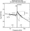 |
Fig. 2. Example of a typical voltage power spectrum around the electron plasma frequency measured by the Wind/WAVES/TNR instrument in the solar wind on June 25, 1995. The solid line is the predicted spectrum fitted to the selected data (in diamonds) among data not retained (dots) for the QTN fitting (see text). The annotations indicate the electron parameters obtained by fitting the theoretical spectrum from the ion and the electron QTN, using a sum of two isotropic Mxwellians – a core “c” and a halo “h” – to the observed spectrum. The vertical line indicate the locations of the local electron plasma frequency obtained by both a Neural Network (“NN”, solid line) and by QTN fit (“fitted”, dashed line). |
The determination of the electron density,  , relies basically on the identification of the “plasma line” at fpe in the QTN spectrum. This is done routinely using a Neural Network (NN) developed by the WAVES team at the Paris Observatory (Richaume 1996; Salem 2000). The plasma frequency is determined with an accuracy of half a channel, which corresponds to a density accuracy of about 4.4%, independently of any calibrations or any model assumptions for the eVDF. These measurements of the NN fpe are routinely archived in the French CDPP (Centre de Données de Physique Spatiale) database.
A more refined but model-dependent way to determine more electron parameters, beyond just the electron density, is the QTN spectroscopy technique (Meyer-Vernet 1979; Meyer-Vernet & Perche 1989; Meyer-Vernet et al. 1998, 2017; Issautier et al. 1999). This method consists of predicting the voltage spectrum measured at the tips of the wire antennas at frequencies much above the local ion characteristic frequencies and the electron gyrofrequency using a model for the eVDF, usually a sum of two isotropic Maxwellians, a core (density Nc and temperature Tc) and a halo (density Nh and temperature Th). The total predicted spectrum around fpe is the sum of the Doppler-shifted proton spectrum (depending on the solar wind proton speed Vsw and temperature Tp) and the electron spectrum (Issautier et al. 1998). Then we fit the measured spectrum to the predicted spectrum to derive the following parameters: total density Ne = Nc + Nh, core temperature Tc, halo-to-core density ratio α = Nh/Nc and halo-to-core temperature ratio τ = Th/Tc. It should be noted that the determination of the density alone is independent of any eVDF model used in the QTN spectroscopy technique. This QTN technique has been implemented on Wind to routinely determine the QTN electron parameters (Salem 2000; Salem et al. 2001, 2003a), using Vsw and Tp measured by the 3DP experiment at 3 s cadence.
Figure 2 shows the QTN fit of the measured spectrum. The diamonds are the measured data points selected for the fit. The NN fpe and the one from the QTN fit agree very well: The total electron density is obtained by the cutoff near the plasma peak, that is its determination can be mainly based on detecting the steepest growth rate (e.g., Meyer-Vernet & Perche 1989; Moncuquet et al. 2020). The value of Tc is mainly determined by both the plateau below the plasma line and the slope of the spectrum above it. The width and amplitude of the plasma line represent a measure of the density and temperature ratios, α and τ, respectively. For the spectrum shown in Fig. 2, Vsw = 761 km s−1 and Tp = 47.5 eV. The QTN fit parameters are: error on the total fit σ = 2.4%, fpe = 22.2(±0.8%),kHz so that Ne = 6.1(±1.6%) cm−3, Tc ≃ 11.5(±10.4%) eV, τ ≃ 5.6(±15.8%) and α = 0.06(±67.3%). As shown in the above example, the QTN technique is robust in yielding an accurate determination of the electron density within 2% and the core temperature within 10%; however, the uncertainties on the suprathermal (halo) density and temperature are much higher due to our underlying assumption of an isotropic Maxwellian in the QTN calculations, which does not account for the halo suprathermal tails or the strahl (Issautier et al. 1998; Meyer-Vernet et al. 1998, 2017).
Both the Neural Network and the QTN fit have routinely been applied to the TNR data in order to obtain electron parameters. So far, NN TNR densities are available from the beginning of the mission in late 1994 until 2020. Electron parameters from the QTN fit are only available from late 1994 to late 2004. These data sets are key to the calibration process of the 3DP eVDF data and to getting a good estimate of Wind’s s/c potential. The QTN technique, by its robustness, has been applied on Ulysses (Maksimovic et al. 1995; Issautier et al. 1998, 2001), and more recently on BepiColombo (Moncuquet et al. 2006), Parker Solar Probe (Maksimovic et al. 2020a; Moncuquet et al. 2020), and Solar Orbiter (Maksimovic et al. 2005a, 2020b).
It should be noted that the longest X antenna was broken twice during the Wind mission, once on August 3, 2000, and again on September 24, 2002 (Malaspina & Wilson 2016). These episodes changed the effective electrical length of the antenna and its response. This affects the level of the QTN power spectrum, but it does not affect the absolute value of the measured cutoff frequency of the plasma line; therefore, it does not change the measured QTN fpe or total electron density Ne, which is the key parameter for the calibrations in this work.
2.3. The SWE Faraday Cup and 3DP ion data
All of the ion (proton and Helium) data from the Wind SWE Faraday Cups have now been analyzed and processed using a sophisticated and adaptive, nonlinear code developed by Maruca (2012). This work has enabled revolutionary studies on the temperature anisotropy instabilities of protons (Kasper et al. 2002; Maruca et al. 2011), and of α-particles (Maruca et al. 2012), as well as ion heating/thermalization (Kasper et al. 2008, 2013; Maruca et al. 2013).
We complement this SWE proton and Helium data set from Wind/SWE with proton data from the proton sensor, PESAL, of the 3DP experiment (Lin et al. 1995). The 3DP proton data set includes continuous 3 s proton moments – density, velocity and temperature.
3. Analysis method of the eVDF
3.1. Data selection criteria
We focus our analysis on the first four years of the Wind mission, namely from January 1, 1995 to December 31, 1998, which correspond to the solar minimum between solar cycles 22 and 23. The starting point of this analysis is to select solar wind intervals, outside the Earth’s magnetosphere and away from the bow shock and the ion/electron foreshock regions. We use a standard model of the bow shock (Slavin & Holzer 1981) to determine when the s/c is outside the shock region and test for magnetic field connectivity to ensure the s/c is outside the foreshock.
Once we identified undisturbed solar wind intervals throughout the Wind mission, we selected all eVDFs available from both EESA-L and EESA-H. We determined one-count levels and removed measured background count rates for both analyzers. For EESA-H, we also removed angular bins that are polluted by solar UV, which tend to be bins in the Sunward direction.
We selected minimum and maximum energy channels for both analyzers. For EESA-L, a minimum of 5–10 eV was considered depending on the detector’s configured minimum energy channel Emin in order to remove the measured photo-electrons. For EESA-H a maximum energy channel was set at 2–3 keV. Above these energies, high-energy super halo electrons dominate the eVDFs (Lin 1998; Wang et al. 2012). The super halo electrons are not considered in this analysis.
3.2. Spacecraft potential
The EESA-L and EESA-H distributions are converted from counts to phase space density using the instrument geometric factor and integration time. The next step is to correct for the effects of s/c potential on the measured eVDFs. We make an initial estimate of the s/c potential based on the measured density from the QTN, using a current balance model that accounts for photo-electrons, solar wind electrons and ions including the effects of their thermal motions and bulk flows (Salem 2000; Salem et al. 2001). The first estimate ϕ0 of the s/c potential uses a photo-electron temperature Tph of 2 eV (see Appendix in Salem et al. 2001).
We then use ϕ0 to correct the energies of the eVDFs: E′ = E − eϕ0. These new energies are then converted into velocities in 3D velocity space, after which we transform them to the solar wind frame in a field aligned coordinate system [v∥, v⊥1, v⊥2]. The solar wind frame is defined as the frame of zero ion current, Ji = Ni Vsw = Np Vp + 2 Nα Vα, where p and α denote protons and α-particles, respectively. We neglect any minor ion contributions.
Our s/c potential correction is isotropic (monopole potential). Pulupa et al. (2014a) consider the case of non-isotropic potentials for the same data set used here and show that the correction is small affects only odd moments. For typical solar wind parameters, the correction is ∼2% in the velocity and ∼4% in the heat flux.
3.3. Gridding and combining EESA-L and EESA-H eVDFs
We grid the data structure for both EESA-L and EESA-H eVDFs using a Delaunay triangulation method (Lee & Schachter 1980) to interpolate a 2D eVDF onto a regularly spaced grid. For this, we symetrize the eVDF with respect to V∥ = 0 under the assumption of gyrotropy and no drifts in the direction perpendicular to the background magnetic field.
We then combine EESA-L and EESA-H structures using the one-count levels for each to cut the eVDF for best overlap. For energies where EESA-L counts are ten times the one-count level or greater, EESA-L data are used. For higher energies, the more sensitive EESA-H detector is used. For a typical eVDF, this transition energy between EESA-L and EESA-H data corresponds to a velocity between 1 × 10⁴ and 2 × 10⁴ km s−1. We test the consistency between EESA-L and EESA-H over their common energy range.
The result is one full eVDF from a few eV to 2–3 keV, sampling core, halo and strahl electrons.
If the approximate s/c potential described in Sect. 3.2 is not the true s/c potential, this will introduce an error in the density moment of the eVDF (Salem et al. 2001). We do a first fit of the combined eVDF and calculate a total density, Ne3DP. Then, we test the accuracy of the s/c potential by comparing this total density to the highly accurate total density from the QTN method, NeTNR. If both densities are not equal, then we initiate an iterative s/c potential estimate and refit the eVDF until both 3DP and TNR density are equal (within a predefined margin), Ne3DP = NeTNR (Pulupa et al. 2014a). Figure 3 illustrates this iterative procedure to determine the true Wind s/c potential ϕ that we use in the final fit process to determine the electron core, halo and strahl parameters. This true Wind s/c potential is retained as the one for which Ne3DP = NeTNR. Salem et al. (2001) provided (in the appendix) an expression of Wind’s s/c potential as a function of electron density from a current balance, and this expression can be used to derive a relationship between the difference in s/c potential and its corresponding error in electron density, which is given by: ΔNe/Ne ∼ Δϕ/Tph. For Tph = 2 eV, a difference of 0.1 Volts in the s/c potential can lead to a 5% error in the density, but the temperature would not be affected.
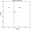 |
Fig. 3. Illustration of the iterative method for determining s/c potential (see text for details). We arrive at an estimated value ϕ of the s/c potential by iterating through various “candidate” s/c potentials, minimizing the difference between the electron density determined as the first-order moment of the eVDF and the electron density obtained from the QTN method. |
3.4. eVDF fit technique
The eVDF fit procedure consists of fitting cuts through the full eVDFs to a model of the solar wind electron distribution that includes two populations, the core and the halo, only. All fits are performed in IDL using a Levenberg–Marquardt least-squares fit technique (Markwardt 2009).
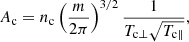
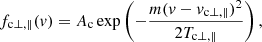
The core is modeled by a drifting bi-Maxwellian distribution fc, characterized by a density nc, parallel and perpendicular drift velocities vc∥ and vc⊥, and parallel and perpendicular temperatures Tc∥ and Tc⊥. The halo is modeled by a drifting bi-κ distribution fh, characterized by a density nh, parallel and perpendicular drift velocities vh∥ and vh⊥, parallel and perpendicular temperatures Th∥ and Th⊥, and a κ-parameter characterizing the high-energy power-law tails of the suprathermal halo (Maksimovic et al. 1997; Štverák et al. 2009). The beam-like strahl population fs is not fitted to a closed function; it is instead defined as the excess in the 2-D distribution function between the measured distribution f and the core+halo model, namely fs = f − fc − fh.
The core “c” and halo “h” electron populations are described by the sum
 (1)
(1)
where
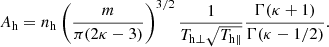
![Mathematical equation: $$ \begin{aligned} f_{\rm c} \,(v_{\parallel },v_{\perp }) = A_{\rm c} \; \exp \left(-\frac{m}{2} \left[ \frac{(v_{\perp }-v_{\mathrm{c} \perp })^2}{T_{\mathrm{c} \perp }} + \frac{(v_{\parallel }-v_{\mathrm{c} \parallel })^2}{T_{\mathrm{c} \parallel }} \right] \right), \end{aligned} $$](/articles/aa/full_html/2023/07/aa41816-21/aa41816-21-eq3.gif) (2)
(2)
 (3)
(3)
![Mathematical equation: $$ \begin{aligned} f_{\rm h}\,(v_{\parallel },v_{\perp }) = A_{\rm h} \; \left\{ 1 + \frac{m}{2\kappa -3} \left[ \frac{(v_{\perp }-v_{\mathrm{h} \perp })^2}{T_{\mathrm{h} \perp }} + \frac{(v_{\parallel }-v_{\mathrm{h} \parallel })^2}{T_{\mathrm{h} \parallel }} \right] \right\} ^{-\kappa -1}, \end{aligned} $$](/articles/aa/full_html/2023/07/aa41816-21/aa41816-21-eq5.gif) (4)
(4)
and
 (5)
(5)
To reduce the number of parameters in a given fit, we apply our fits separately to perpendicular and parallel cuts through 1D distribution functions
 (6)
(6)
where
 (7)
(7)
![Mathematical equation: $$ \begin{aligned} f_{\mathrm{h} \perp , \parallel }(v) = A_{\rm h} \; \left[ 1 + \frac{m}{2\kappa -3} \frac{(v-v_{\mathrm{h} \perp , \parallel })^2}{T_{\mathrm{h} \perp , \parallel }} \right]^{-\kappa -1}, \end{aligned} $$](/articles/aa/full_html/2023/07/aa41816-21/aa41816-21-eq9.gif) (8)
(8)
where the parallel and perpendicular subscripts have been eliminated. We use a common form for both parallel and perpendicular cuts:
![Mathematical equation: $$ \begin{aligned} f = A_0 \exp \left( - \frac{(v - A_1)^2}{A_2} \right) + A_3 \left\{ 1 + \left[ \frac{(v - A_4)^2}{A_5} \right]^{-A_6} \right\} . \end{aligned} $$](/articles/aa/full_html/2023/07/aa41816-21/aa41816-21-eq10.gif) (9)
(9)
In both the perpendicular and parallel directions, there are seven fit parameters. Starting each fit with a reasonable initial guess improves the speed and stability of the algorithm. For the perpendicular case, the fit is initialized using the TNR measurements of the core and halo density and temperature. The starting guess for the κ parameter is based on solar wind speed (κ = 6 if Vsw < 500 km s−1, κ = 5 if 500 < Vsw < 650 km s−1, and κ = 4 if Vsw > 650 km s−1) from previous experience. The drift velocity parameters A1 and A4 are fixed at zero (consistent with the gyrotropic assumption), reducing the number of fit parameters to 5.
The perpendicular fit determines perpendicular temperature (from A2 and A5), the κ value from A6, and the overall phase space amplitude of the core and halo populations A0 and A3. The parallel fit is performed after the perpendicular fit, keeping A0, A3, and A6 constant. The parallel fit determines the core and halo drift speed A1 and A4, and the parallel temperatures (from A2 and A5). Using the measured amplitudes A0 and A3 and the measured temperature and κ, the core and halo densities can be determined.
Figure 4 shows two typical eVDFs in the solar wind at 1 au measured by the Wind/3DP electrostratic analyzers EESA-L and EESA-H. The left panels (a) and (c) show an eVDF in the slow solar wind (at 1995-06-19/00:06:38), and the right panels (b) and (d) show an eVDF in the fast solar wind (at 1995-06-19/23:13:59). The top panels (a) and (b) show cuts through the eVDF in one of the two directions perpendicular to the local magnetic field B: the diamonds are data points from EESA-L and the asterisks from EESA-H. The dotted lines represent the one-count level for EESA-L and EESA-H. The blue dashed line in Figs. 4a and 4b represents the sum of Maxwellian and Kappa distributions calculated using the QTN fit parameters (indicated in blue). The red line in Figs. 4a and 4b represents the fit to the measured perpendicular eVDF cut; the resulting fit parameters are indicated in red. The bottom panels (c) and (d) show cuts through the eVDF in the direction parallel to B. The perpendicular fit is reported in red, and the perpendicular fit parameters are used to initialize the parallel eVDF fit.
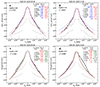 |
Fig. 4. Two typical eVDFs measured by EESA-L and EESA-H at 1 au in the slow solar wind – panels (a) and (c) –, and in the fast solar wind – panels (b) and (d). The top panels (a) and (b) show cuts through the eVDF in one of the two directions perpendicular to the local magnetic field B: the diamonds are data points from EESA-L and the asterisks from EESA-H. The dotted lines represent the one-count levels for EESA-L and EESA-H. The blue dashed line represents the sum of Maxwellian and κ-distributions calculated using the QTN fit parameters (indicated in blue), which are used to initialize the eVDF fit. The red line represents the fit to the measured perpendicular eVDF cut; the resulting fit parameters are indicated in red. The bottom panels (c) and (d) show cuts through the eVDF in the direction parallel to B. The perpendicular fit is reported in red, and the perpendicular fit parameters are used to initialize the parallel eVDF fit, the results of which are given in green. In each plot, the points that are selected for inclusion in the eVDF fit are filled with pink color. |
As shown in Figs. 4c and 4d, the points that are selected for inclusion in the eVDF parallel fit are filled with pink color. Points that are determined by the algorithm to represent the strahl and points close to the one-count level are not included in the eVDF fit. The result of the parallel fit is indicated in green (green curves and green parameters). The solar wind speed and s/c potential retained by the algorithm are given on the top of each panels, as well as a quality measure of the nonlinear least-square fit (see Sect. 3.7) and its χ2.
3.5. Extracting the electron Strahl
After the final perpendicular and parallel eVDF fit described in Fig. 4, fmodel(v⊥, v∥) is the 2D distribution function constructed from the perpendicular and parallel fit parameters, not including strahl, in other words, a core-halo model.
The combined EESA-L and EESA-H distributions encompass over 10 orders of magnitude in phase space density. Therefore, detection of a feature such as the strahl, in comparison to a difference between the measured distribution fdata and the model fmodel due to “noise”, requires the use of a normalized distribution. We define the Δ distribution as the normalized difference between fdata and fmodel:
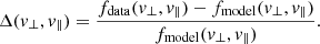 (10)
(10)
From Δ(v⊥, v∥), we extract perpendicular and parallel cuts. Values of the perpendicular cut, Δ(v⊥, v∥ = 0), are indicated in blue in Fig. 5 and are typically small (less than 1) because the strahl is not present in the perpendicular cut. In contrast, values of the parallel cut, Δ(v⊥ = 0, v∥), indicated in red in Fig. 5, can reach high values, revealing clearly the strahl and its shape. The strahl structures shown in Fig. 5 are typical of those observed by Wind in the unperturbed solar wind: the strahl is uni-directional with a peak density (relative to the core/halo density) at a parallel speed between 1 × 10⁴ and 2 × 10⁴ km s−1, and is limited in velocity/energy with a cutoff at usually less than 4 × 10⁴ km s−1.
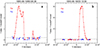 |
Fig. 5. Illustration of the algorithm used to extract the strahl from the eVDFs of Fig. 4; the left panel (a) shows the slow wind eVDF and the right panel (b) shows the fast wind eVDF. Cuts through the Δ distribution (see text) in the parallel and perpendicular direction are indicated in red and blue, respectively. The obvious peak in the parallel cut in red shows the range and structure of the strahl. In the fast wind, the strahl is much more prominent than in the slow wind. However, the strahl is wider in the slow wind than in the fast wind. The dashed horizontal line represents the threshold for the automated extraction of the strahl. |
The dashed horizontal line in Fig. 5 represents a threshold for the automated extraction of the strahl. For each eVDF, this threshold is determined using the perpendicular cut as a control (assuming that the perpendicular cut contains no strahl): values of the Δ-distribution in the parallel direction that have values significantly greater than typical values in the perpendicular cut are counted as strahl. The obvious peak in the parallel cut in red shows the range and structure of the strahl. In the fast wind, the strahl is much more prominent than in the slow wind. Indeed, Δ ∼ 3 for the slow wind example (left panel a) and Δ ∼ 30 for the fast wind example (right panel b), that is, ten times higher. However, the strahl is wider in the slow wind than in the fast wind.
To extract the 2D strahl distribution from the measured fdata, we select all data points characterized by Δ > δ0, where δ0 is a set threshold, and define the strahl distribution as the difference between the measured eVDF and the core-halo model:
 (11)
(11)
Once the 2D strahl distribution is extracted, we characterize it by integrating strahl moments, namely density, bulk speed (in the solar wind frame), intrinsic parallel and perpendicular temperatures, as well as heat flux. Figure 6 shows the 2D strahl distribution for the above examples of slow and fast wind (left -a- and right -b- panels, respectively). The strahl moments are also given.
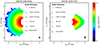 |
Fig. 6. 2D distribution of the strahl after extraction from the total observed eVDF. The left panel (a) and the right panel (b) are the same slow and fast solar wind examples as in Figs. 4 and 5. The calculated strahl moments for each example are listed. |
In these representative examples, the strahl is not only wider in energy range but also broader in pitch angle in the slow wind compared to the fast wind. The temperature anisotropy of the strahl, determined from the intrinsic parallel and perpendicular temperatures (i.e., calculated in its own frame) yield a good a characterization of its angular width. In the example of Fig. 6, the temperature anisotropy is 1.26 for the fast wind (right panel) and 2.70 for the slow wind (left panel), confirming that the strahl is broader in the slow wind compared to the fast wind.
3.6. Total electron moments and heat flux
The eVDF fit process described above yields independent parameters of the core, halo and strahl populations for each measured, processed and corrected distribution function. In addition to the core, halo and strahl thus determined, we also integrate each full and calibrated eVDF up to the energies of the super halo to determine the total electron density ne, parallel and perpendicular temperatures Te∥ and Te⊥, as well as the electron heat flux Qe. By construction, this total heat flux is simply the parallel heat flux  , since the eVDF is symmetric in the perpendicular direction within the gyrotropy assumption. During this process, we verify that ne thus determined is consistent with nc + nh + ns as determined above.
3.7. Quality assessment of eVDF fits
The quality of each eVDF fit is evaluated once the fit procedure is complete. The quality factor is a numerical measure with values between 0 (worst) and 10 (best), based on the convergence of the fit algorithm, the reported χ2 value of the parallel and perpendicular fits, the agreement between EESA-L and EESA-H over their common energy range, sufficient density of angular bins in the vicinity of the strahl, and independently measured quality of the QTN measurements used to initialize the fit. Times when the EESA detectors are not in a suitable mode for analysis are also eliminated. For example, during certain intervals the integration time for EESA-H is set too low to accumulate sufficient statistical counts in the strahl energy range; in these cases (only a few percent), the resulting overlap between EESA-L and EESA-H is not good. The remainder of this paper is based on 280 000 full eVDF fits that were determined to be sufficiently high quality.
It is worth emphasizing that the eVDF fits, as shown in Fig. 4, are very robust for two main reasons: (a) they are constrained to fewer free paramaters by performing separate perpendicular and parallel fits, with the key condition Ne = NQTN considered as the true total electron density. We do not have to rely on very accurate initial – Tc, α and τ – parameters from the TNR for the eVDF fits to converge, as shown in the examples of Fig. 4. (b) the combination of EESA-L and EESA-H up to 2 keV adds to the robustness of the eVDF fits via stronger constraints to the halo parameters Th and κ due to the extra data points above the strahl energies, and therefore to the strahl parameters since the strahl is defined as the difference between the measured eVDF and the core-halo model. Indeed, the uncertainties of the eVDF fit parameters are: ΔNc ∼ 4%, ΔTc ∼ 2%, ΔNh ∼ 10 − 15%, ΔTh ∼ 3% and Δκ ∼ 3%. The uncertainties on the drift velocities of both the core and the halo are within 5% of their respective thermal speeds.
4. Results
The application of the algorithm layed out in Section 3 to our 280 000 eVDFs creates a large data set of plasma parameters for the total electron species and the core, halo and strahl populations (Salem & Pulupa 2023). In this section, we present a first statistical analysis of these parameters. The underlying statistics are also summarized in the Appendix.
Figure 7 shows the probability distribution of solar wind bulk speeds in our full data set. The black histogram shows the distribution of Vsw resulting from our eVDF fits. The binning in solar wind speed uses a binsize of 5 km s−1 between 250 and 800 km s−1. The red histogram shows the distribution of the same parameter, Vsw, sampled from the original 3-second proton 3DP data (onboard moments) from the same 4-year time period, normalized to the maximum of the eVDF histogram. The proton histogram is based on 1.7 million data points. The comparison between the electron histogram and the proton histogram shows that our eVDF processing does not introduce any bias in our sampled distribution of solar-wind speeds compared to the 3DP proton data. Among the 280 000 eVDFs in our 4-year sample, 86.1% are in the slow solar wind (Vsw ≤ 500 km s−1) and 13.9% are in the fast wind (Vsw > 500 km s−1), which is typical of the solar wind in the Ecliptic plane at solar minimum (McComas et al. 2000; Smith et al. 2003).
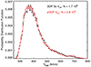 |
Fig. 7. Probability distributions of the solar wind speed Vsw. The black histogram represents the distribution based on our eVDF analysis, and the red histogram represents the distribution based on 3DP onboard proton moments, normalized to the maximum of the eVDF historgram. |
For the statistical analysis of solar wind electron data at 1 au, we now summarize our data analysis in column-normalized 2D histograms of electron parameters from the integration and/or fit of the final combined (EESA-L and EESA-H) eVDFs, corrected for s/c potential effects in Figs. 8 through 16. We chose the solar wind speed as a reliable statistical ordering parameter for the histograms in Figs. 8 through 15. We applied the same bin widths to the following histograms as in Fig. 7, namely, a binsize of 5 km s−1. The color bar represents the logarithm of the number of counts per bin, normalized to the maximum number of counts per bin in each column. The black circles mark the peak centroid in each column, and the black vertical lines represent the half-width or standard deviation based on a Gaussian fit to the normalized values in each column (see Appendix).
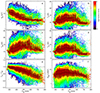 |
Fig. 8. Column-normalized 2D histrograms of parameters of the total electron species: (a) electron density Ne, (b) total electron temperature Te, (c) temperature Te∥ of the total electron distribution in the direction parallel to the mean magnetic field, (d) temperature Te⊥ of the total electron distribution in the direction perpendicular to the mean magnetic field, (e) temperature ratio Te⊥/Te∥ of the total electron distribution, and (f) magnitude of the parallel heat flux |Qe∥| of the total electron distribution. |
4.1. Statistics of the total electron distribution
Figure 8 displays histograms of the moments of the total electron distribution function, not separated by core, halo, or strahl. Panel (a) shows the distribution of the total electron density, Ne. The average Ne drops from ∼13 cm−3 in slow wind to ∼4 cm−3 in fast wind. Also, the variability in Ne decreases with increasing Vsw. Panel (b) shows the total electron temperature Te. Although the analysis suggests some variation with wind speed, the statistical trend is less pronounced than the trend in Ne. For most cases, the total electron temperature varies between ∼8 eV and ∼16 eV. However, we also see a larger variation in Te at smaller Vsw than at large Vsw. Panels (c) and (d) show the temperatures Te⊥ and Te∥ of the total electron population perpendicular and parallel with respect to the background magnetic field, respectively. Like in the case of the total Te, Te∥ and Te⊥ show more variation in fast wind than in slow wind. We especially see that Te⊥ assumes smaller average values in the fast wind (∼8 eV) compared to the slow wind (∼12 eV). Panel (e) confirms this statistical trend by showing the histogram for the ratio Te⊥/Te∥. The total eVDF is less anisotropic in slow wind and exhibits an average anisotropy of Te⊥/Te∥ ∼ 0.7 in fast wind. Panel (f) shows the magnitude of the parallel heat flux |Qe∥| of the total electron heat flux. |Qe∥| exhibits more variation and a slightly higher value in slow solar wind (∼ 4 μW/m2) than in fast solar wind (∼ 3 μW/m2).
Figure 9 shows the statistical results for the proton data and derived parameters for the total eVDFs in our data set. Panel (a) shows that the proton temperature follows a clear positive trend with Vsw, which is a well-known property of the solar wind (Burlaga & Ogilvie 1970, 1973; Lopez & Freeman 1986). The temperature increases from ∼2 eV in slow wind to ∼24 eV in fast wind. This increase in Tp, combined with the Vsw dependence of Te shown in Fig. 8b, explains the strong anticorrelation between Te/Tp and Vsw seen in panel (b). The total proton and electron temperatures are on average approximately equal for Vsw ∼ 530 km s−1. Panels (c) and (d) show the ratios between the total proton and electron thermal energy densities and the magnetic-field energy density, respectively, which we calculate as βp = 8πnpkBTp/B2 and βe = 8πnekBTe/B2, where kB is the Boltzmann constant. We see that βp ≲ 1 on average with only a slight dependence on Vsw, while βe shows, on average, a clear anticorrelation with Vsw. We find that βe ∼ 1 for Vsw ∼ 450 km s−1. We note that fast wind exhibits less variability in both βp and βe compared with slow wind.
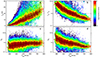 |
Fig. 9. Column-normalized 2D histrograms of proton parameters and derived total electron parameters: (a) total proton temperature Tp, (b) temperature ratio Te/Tp of the total proton and electron distributions, (c) βp of the total proton distribution, and (d) βe of the total electron distribution. |
4.2. Statistics of core, halo, and strahl components
Figure 10 shows column-normalized histograms for the electron core parameters as functions of Vsw. Panel (a) shows the core number density Nc. On average, Nc varies from ∼12 cm−3 in slow solar wind to ∼4 cm−3 in fast solar wind. Likewise, the variability in Nc decreases with increasing Vsw. Panel (b) shows the drift speed Vdc between the electron core and the protons, multiplied with the sign of Qe∥. By multiplying Vdc with sign(Qe∥), we correct for the sign ambiguity due to the choice of our coordinate system. If Vdc sign(Qe∥) < 0, the core bulk velocity is directed toward the Sun in the coordinate system centered on the proton bulk velocity, and vice versa. We find indeed that Vdc sign(Qe∥) < 0. In the slow wind, |Vdc| is smaller (∼20 km s−1) than in the fast wind (∼100 km s−1). Panels (c) and (d) show the core temperatures in the directions parallel (Tc∥) and perpendicular (Tc⊥) with respect to the magnetic field. Both temperatures are greater in the slow solar wind (Tc∥ ∼ Tc⊥ ∼ 10 eV) than in the fast solar wind (Tc∥ ∼ 8 eV, Tc⊥ ∼ 7 eV). The scalar core temperature Tc reflects the same trend, as shown in panel (e). Consistent with the behavior of Tc∥ and Tc⊥, the temperature ratio T⊥/T∥ of the core decreases from isotropy in slow wind to a value of ∼0.83 in fast wind.
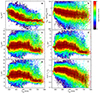 |
Fig. 10. Column-normalized 2D histrograms of electron core parameters: (a) core density Nc, (b) sign-corrected drift speed Vdc sign(Qe∥) between core and proton bulk velocity, (c) temperature Tc∥ of the core in the direction parallel to the mean magnetic field, (d) temperature Tc⊥ of the core in the direction perpendicular to the mean magnetic field, (e) total temperature Tc of the core, and (f) temperature ratio T⊥/T∥ of the core. |
Figure 11 shows the same histograms as Fig. 10, but for the halo instead of the core. Panel (a) shows the halo density Nh, which is mostly independent of Vsw with a value of ∼0.3 cm−3. The halo drift Vdh is directed away from the Sun and assumes values of ∼400 km s−1 in slow solar wind and almost vanishes in fast solar wind. There is evidence for a Sunward halo drift at Vsw ≳ 700 km s−1; however, the statistics for Vdc in this regime is less reliable than at smaller Vsw. A visual inspection of the individual fits (like those shown in Fig. 4) confirms the direction of the drifts – sunward core and halo drifts – and the goodness of the fit overall. Panels (c) and (d) show the halo temperatures in the directions parallel (Th∥) and perpendicular (Th⊥) with respect to the magnetic field. Both temperatures are approximately constant (Th∥ ∼ 53 eV and Th⊥ ∼ 50 eV) in slow solar wind and drop to Th∥ ∼ 32 eV and Th⊥ ∼ 30 eV in fast wind. The constant-temperature regime occurs at Vsw ≲ 600 km s−1. The scalar halo temperature also follows this trend from ∼50 eV in slow wind to ∼32 eV in fast wind. The ratio T⊥/T∥ of the halo is on average less than one, with a slight inverse trend with Vsw on average. We note, however, that there is a large variation in T⊥/T∥ of the halo, so that there are significant times with T⊥/T∥ ≳ 1, especially during slow wind times.
Figure 12 shows the same histograms as Fig. 10, but for the strahl instead of the core. Panel (a) shows the strahl density Ns, which varies from ∼0.04 cm−3 in slow wind to ∼0.08 cm−3 in fast wind. The slow wind shows more variability in Ns than the fast wind. Panel (b) shows the drift speed Vs of the strahl multiplied by sign(Qe∥). The strahl is directed away from the Sun and exhibits an approximately constant average drift speed of ∼4700 km s−1 in the proton frame. Also, the width of the column-normalized data distribution is mostly independent of Vsw. Panel (c) shows the strahl temperature Ts∥ in the direction parallel to the mean magnetic field. Ts∥ ∼ 14 eV on average and is mostly constant with Vsw. On the contrary, the strahl temperature Ts⊥ in the direction perpendicular to the mean magnetic field shows a large variation and a strong anticorrelation with Vsw on average (see panel (d)). While the average Ts⊥ ∼ 30 eV in slow wind, it is ∼15 eV in fast wind. Consequently, the scalar strahl temperature Ts, shown in panel (e), also decreases with increasing Vsw from ∼24 eV in slow wind to ∼15 eV in fast wind. Panel (f) illustrates that the temperature ratio T⊥/T∥ of the strahl varies from ∼3 in the slow solar wind to ∼1.4 in fast wind. As mentioned in Sect. 3.5, Ts⊥/Ts∥ is a good parameter to characterize the angular width of the strahl, and this angular width of the strahl displays a linear anticorrelation with solar wind speed at 1 au.
4.3. Current balance
As an independent check of the density and drift-speed measurements, we analyze the current-balance condition of our fit results for the eVDF in Fig. 13. We show a column-normalized histogram of the quantity Nc Vdc + Nh Vdh + Ns Vs as a function of Vsw. In the proton rest frame, current balance is fulfilled when this quantity is zero. As expected, the results in Fig. 13 are consistent with current balance.
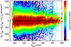 |
Fig. 13. Current balance of the total electron distribution function. |
4.4. Intercorrelations between electron parameters
Since most of the parameters shown thus far exhibit large variability in our histograms, it is not directly possible to deduce ratios between these parameters from the histograms. Instead, the ratios between electron parameters can follow largely independent trends with Vsw. In this section, we analyze some of these ratios to study intercorrelations between a selection of electron parameters.
Figure 14 shows the ratios between the densities of the three electron components from our fit results as functions of Vsw. Panel (a) shows the ratio between the halo density Nh and the core density Nc. We find an increase in Nh/Nc with Vsw from ∼0.02 in slow wind to ∼0.08 in fast wind. Panel (b) shows the ratio between the strahl density Ns and the core density Nc. It increases with Vsw from ∼0.003 in slow wind to ∼0.02 in fast wind. Panel (c) displays the ratio between the strahl density Ns and the halo density Nh. Similar to the ratios shown in panels (a) and (b), this ratio increases with Vsw from ∼0.2 in slow wind to ∼0.4 in fast wind.
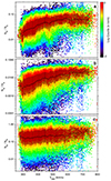 |
Fig. 14. Density ratios of the electron components as functions of Vsw. (a) Nh/Nc, (b) Ns/Nc, and (c) Ns/Nh. |
Figure 15 shows ratios between the scalar temperatures of the electron core, halo, and strahl populations as functions of Vsw. Panel (a) shows the ratio between the scalar halo temperature Th and the scalar core temperature Tc. This ratio is largely independent of Vsw and assumes a value of ∼5 on average. We note that there is a slight increase in Th/Tc to ∼6 in the narrow regime with Vsw ≲ 300 km s−1. Outside of this regime, the variability of Th/Tc is mostly independent of Vsw. Panel (b) shows the ratio between the scalar strahl temperature Ts and the scalar core temperature Tc. This ratio slowly decreases with increasing Vsw from ∼2.8 in slow wind to ∼2 at Vsw ≳ 550 km s−1. Panel (c) shows the ratio between the scalar strahl temperature Ts and the scalar halo temperature Th. Like the other temperature ratios in Fig. 15, Ts/Th shows only a small variation with Vsw. It assumes a value of ∼0.4.
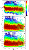 |
Fig. 15. Ratios of the scalar temperatures of the electron components as functions of Vsw. (a) Th/Tc, (b) Ts/Tc, and (c) Ts/Th. |
Figure 16 shows histograms of ratios between the scalar temperatures of the electron components as functions of their density ratios. These diagrams illustrate intercorrelations between the plotted quantities. Although we do not use Vsw in Fig. 16, we still apply column-normalization and determine averages and standard deviations as in Figs. 8 through 16. Panel (a) shows the correlation between Th/Tc and Nh/Nc. We see a clear trend from Th/Tc ∼ 8 at Nh/Nc ∼ 0.003 to Th/Tc ∼ 4 at Nh/Nc ∼ 0.2 with a small variability in each bin. Panel (b) shows the correlation between Ts/Tc and Ns/Nc. These two ratios exhibit a less pronounced intercorrelation compared to the ratios shown in panel (a). We also note that the variability decreases with increasing Ns/Nc. The average Ts/Tc slightly increases from ∼1.3 at Ns/Nc ∼ 0.0003 to ∼2.3 at Ns/Nc ∼ 0.05. Panel (c) displays the relationship between Ts/Th and Ns/Nh. The average ratio Ts/Th increases from ∼0.1 at Ns/Nh ∼ 0.01 to ∼0.5 at Ns/Nh ∼ 0.4, and then decreases again to ∼0.3 at Ns/Nh ∼ 2.
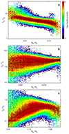 |
Fig. 16. Intercorrelations between electron temperature ratios and density ratios. (a) Th/Ts as a function of Nh/Nc, (b) Ts/Tc as a function of Ns/Nc, and (c) Ts/Th as a function of Ns/Nh. |
5. Discussion
The total electron parameters in our data set (Salem & Pulupa 2023) according to Fig. 8 are largely consistent with the known behavior in the solar wind. Fast wind exhibits significantly smaller electron densities (and thus, per quasi-neutrality, significantly smaller ion densities) than the slow solar wind. Our data set also confirms that Te is generally smaller in fast-wind streams compared to slow wind (Ogilvie et al. 2000; Wilson 2018). However, Te is highly variable in the slow solar wind, showing a general correlation with Vsw in the slow solar wind up to ∼550 km s−1 and an anticorrelation with Vsw in the fast solar wind above 550 km s−1 (Maksimovic et al. 2020a). It is interesting to note that the proton temperature shows an opposite and more pronounced trend (see Fig. 9). This opposite behavior of Te and Tp leads to a strong dependence of Te/Tp on Vsw. The ratio Te/Tp is of great interest for local plasma processes since, for example, the damping rate of ion-acoustic waves and the energy partitioning of plasma heating are very sensitive to this parameter (Howes et al. 2006; Schekochihin et al. 2009, 2019; Kawazura et al. 2019, 2020). We also note that the density and temperature behavior cause a significant dependence of the average βe on Vsw, which is more pronounced than the dependence of βp on Vsw. This trend causes the average βe to cross the βe = 1 line between slow and fast wind streams.
In general, fast solar wind exhibits more non-equilibrium features in our data set than slow solar wind. For instance, the total eVDF as well as the core and (to a lesser extent) halo components exhibit more temperature anisotropy in fast wind than in slow wind (Figs. 8, 10, and 11). Also, the core drift is more pronounced in the fast solar wind than in slow solar wind. These results suggest that collisions, which occur more often in slow wind, likely play a role in the reduction of non-equilibrium kinetic features in the eVDF. In particular, collisions lead to a stronger effect in the core distribution than in the halo distribution.
While the average trends in the halo temperatures largely mirror the average trends in the core temperatures (Fig. 11), the halo density is mostly constant, and the core-halo drift exhibits larger values in slow solar wind. The core-halo-strahl drift guarantees current balance (see Fig. 13). The current contribution due to the Sunward core drift is compensated for by the anti-Sunward halo and strahl drifts. The halo is on average only slightly anisotropic with T⊥ < T∥, which may be a consequence of the often suggested connection between strahl and halo electrons.
According to Fig. 12, the strahl shows only small variations in Ns, Vs sign(Qe∥), and Ts∥ as functions of Vsw. However, Ts⊥ (and thus Ts and T⊥/T∥ of the strahl) show a strong anticorrelation with Vsw on averge. These trends are consistent with the scenario of local scattering of strahl electrons toward larger v⊥ (Maksimovic et al. 2005b; Štverák et al. 2009; Vasko et al. 2019; Verscharen et al. 2019a). In slow wind, the travel time of a plasma parcel from the Sun to 1 au is longer than in fast wind, so that the scattering processes can act on the strahl electrons for a longer time as a possible explanation for the observed trend. This scattering scenario is also in agreement with Fig. 14b and (to some extent) with Fig. 14c, which show that the relative strahl density is lower in the slow wind than in the fast wind, consistent with the scattering of strahl electrons into the halo. As a caveat to this interpretation, we note that the observed ratio of halo-to-core density (Nh/Nc) also increases with Vsw, which suggests that other processes in addition to strahl scattering lead to a Vsw-independent trend in Nh even though Nc changes significantly with Vsw. In this context, we note that the temperature ratios between the electron components are mostly independent of Vsw (see Fig. 15), a constraint that must be fulfilled by kinetic models explaining the partitioning of particles and energies between core, halo, and strahl.
Figure 16 shows further interesting correlations between temperature ratios and density ratios of the electron components. Especially, panel (a) suggests that there is a clear correlation between Th/Tc and Nh/Nc, which requires a theoretical explanation.
One important common property seen in all the 2D histograms presented in Figs. 8–15 that is worth discussing is the large half-widths of the distribution around the peak centroid. These large fluctuations of the various electron parameters that we determined are not a reflection of the uncertainties on their determination (see Sect. 3.7). They are a reflection of the natural variability of the solar wind. This variability of the solar wind is a physical fact that we want to measure. Now, our electron measurements are accurate enough to show that variability. Indeed, the 2D histograms show statistics of fluctuations at timescales of 96 s (cadence of the availibility of the measured eVDFs) and longer. The key point is that at these timescales the fluctuations do not reflect the uncertainties in each measurement (3 s being the acquisition time of each eVDF). Solar wind proton density and temperature have been observed to display natural variability at scales larger than their measurement cadence, albeit smaller than that of electromagnetic fields and/or solar wind velocity (e.g., Salem et al. 2003a, 2009; Bruno & Carbone 2013; Verscharen et al. 2019b). The electron core, halo and strahl properties show properties. Perhaps the most peculiar one concerns the variability of the strahl temperatures Ts∥ and Ts⊥ (Fig. 12): Ts∥ displays a much smaller variability than Ts⊥. This property could be a reflection of pitch-angle scattering processes that diffuse and broaden the strahl, even more so in the slow wind than in the fast wind.
6. Conclusions
This paper presents a comprehensive analysis of the structure of the eVDF in the ambient solar wind at 1 au, using data from the 3DP and the WAVES experiment on board NASA’s Wind s/c up to energies of 2-3 keV. The combination of data from the electrostatic analyzers measuring the actual eVDF and from the wave receivers measuring the quasi-thermal noise of the plasma led to good estimates of Wind’s s/c electrical potential (Salem et al. 2001; Pulupa et al. 2014a), an unknown quantity otherwise.
The correction for the s/c potential allows us to extract accurate properties of the eVDF in the solar wind. The properties of the three main electron populations in this energy range – the core, halo and strahl – are statistically characterized in great detail in the slow and fast solar wind. The core and halo populations are modeled by the sum of a bi-Maxwellian distribution and a bi-κ distribution, respectively. The fit of the core-halo model to the observed distribution leads to a complete characterization of the core and halo populations. The strahl is extracted by substracting the core-halo model from the observed distributions, allowing us to integrate the strahl moments. In this way, we obtain a set of moments and parameters for each population including temperature anisotropies and heat fluxes.
Our data analysis algorithm is automated with the goal of analyzing several years worth of data statistically and building a database of accurate core, halo and strahl parameters in the solar wind. We here present statistics based on our initial four-year data set (1995–1998). This is to-date the best high-precision, large-scale electron data set of the pristine solar wind (Salem & Pulupa 2023). This data set has already enabled further studies (Bale et al. 2013; Pulupa et al. 2014a,b; Tong et al. 2015; Chen et al. 2016; He et al. 2018; Yoon et al. 2019; Verscharen et al. 2019a). Our aim is to apply this technique to the entire 27 years of Wind data yielding the best electron data set of almost two and half solar cycles in the pristine solar wind at 1 au. However, this extension requires a careful reevaluation of the microchannel-plate degradation over the course of the mission, which is beyond the scope of this work. In addition, the 27-year data set will potentially include solar-cycle variations that introduce additional long-time variations to the statistical measures presented in this paper. Such a data set will be a valuable reference for electron research in the context of ongoing electron measurements with the latest heliospheric space missions Parker Solar Probe and Solar Orbiter.
Acknowledgments
This work was supported by NASA grant NNX16AI59G and by NSF SHINE grants 1622498 and 2203319. D.V. is supported by STFC Ernest Rutherford Fellowship ST/P003826/1 and STFC Consolidated Grants ST/S000240/1 and ST/W001004/1. The authors encourage and invite direct collaborations using the dataset presented in this paper, which is available at SPDF under https://doi.org/10.48322/rgf7-3h67, as yearly files. This work was discussed in depth at the ESAC Solar Wind Electron Workshop in May 2019, which was supported by the Faculty of the European Space Astronomy Centre (ESAC).
References
- Acuña, M. H., Ogilvie, K. W., Baker, D. N., et al. 1995, Space Sci. Rev., 71, 5 [Google Scholar]
- Anderson, B. R., Skoug, R. M., Steinberg, J. T., & McComas, D. J. 2012, J. Geophys. Res. (Space Phys.), 117, A04107 [NASA ADS] [Google Scholar]
- Bale, S. D., Pulupa, M., Salem, C., Chen, C. H. K., & Quataert, E. 2013, ApJ, 769, L22 [Google Scholar]
- Berčič, L., Maksimović, M., Landi, S., & Matteini, L. 2019, MNRAS, 486, 3404 [Google Scholar]
- Berčič, L., Larson, D., Whittlesey, P., et al. 2020, ApJ, 892, 88 [Google Scholar]
- Berčič, L., Landi, S., & Maksimović, M. 2021, J. Geophys. Res. (Space Phys.), 126, e28864 [Google Scholar]
- Boldyrev, S., & Horaites, K. 2019, MNRAS, 489, 3412 [Google Scholar]
- Bougeret, J.-L., Kaiser, M. L., Kellogg, P. J., et al. 1995, Space Sci. Rev., 71, 231 [CrossRef] [Google Scholar]
- Bruno, R., & Carbone, V. 2013, Liv. Rev. Sol. Phys., 10, 2 [Google Scholar]
- Burlaga, L. F., & Ogilvie, K. W. 1970, ApJ, 159, 659 [NASA ADS] [CrossRef] [Google Scholar]
- Burlaga, L. F., & Ogilvie, K. W. 1973, J. Geophys. Res., 78, 2028 [NASA ADS] [CrossRef] [Google Scholar]
- Cattell, C., Breneman, A., Dombeck, J., et al. 2021, ApJ, 911, L29 [Google Scholar]
- Chen, C. H. K., Matteini, L., Schekochihin, A. A., et al. 2016, ApJ, 825, L26 [NASA ADS] [CrossRef] [Google Scholar]
- Cranmer, S. R. 2009, Liv. Rev. Sol. Phys., 6, 3 [Google Scholar]
- Cully, C. M., Ergun, R. E., & Eriksson, A. I. 2007, J. Geophys. Res. (Space Phys.), 112, A09211 [Google Scholar]
- Dreicer, H. 1959, Phys. Rev., 115, 238 [NASA ADS] [CrossRef] [Google Scholar]
- Dreicer, H. 1960, Phys. Rev., 117, 329 [NASA ADS] [CrossRef] [Google Scholar]
- Feldman, W. C., Asbridge, J. R., Bame, S. J., Montgomery, M. D., & Gary, S. P. 1975, J. Geophys. Res., 80, 4181 [Google Scholar]
- Feldman, W. C., Asbridge, J. R., Bame, S. J., Gary, S. P., & Montgomery, M. D. 1976, J. Geophys. Res., 81, 2377 [NASA ADS] [CrossRef] [Google Scholar]
- Fitzenreiter, R. J., Ogilvie, K. W., Chornay, D. J., & Keller, J. 1998, Geophys. Res. Lett., 25, 249 [NASA ADS] [CrossRef] [Google Scholar]
- Fuchs, V., Cairns, R. A., Lashmore-Davies, C. N., & Shoucri, M. M. 1986, Phys. Fluids, 29, 2931 [NASA ADS] [CrossRef] [Google Scholar]
- Garrett, H. B. 1981, Rev. Geophys. Space Phys., 19, 577 [CrossRef] [Google Scholar]
- Gary, S. P. 1993, in Theory of Space Plasma Microinstabilities, ed. S. Peter Gary (Cambridge, UK: Cambridge University Press), 193, ISBN 0521431670 [Google Scholar]
- Gary, S. P., & Saito, S. 2007, Geophys. Res. Lett., 34, 14111 [NASA ADS] [CrossRef] [Google Scholar]
- Gary, S. P., Feldman, W. C., Forslund, D. W., & Montgomery, M. D. 1975, Geophys. Res. Lett., 2, 79 [CrossRef] [Google Scholar]
- Gary, S. P., Scime, E. E., Phillips, J. L., & Feldman, W. C. 1994, J. Geophys. Res., 99, 23391 [Google Scholar]
- Gary, S. P., Skoug, R. M., & Daughton, W. 1999, Phys. Plasmas, 6, 2607 [Google Scholar]
- Génot, V., & Schwartz, S. 2004, Ann. Geophys., 22, 2073 [CrossRef] [Google Scholar]
- Goertz, C. K. 1989, Rev. Geophys., 27, 271 [NASA ADS] [CrossRef] [Google Scholar]
- Gosling, J. T., Skoug, R. M., & Feldman, W. C. 2001, Geophys. Res. Lett., 28, 4155 [NASA ADS] [CrossRef] [Google Scholar]
- Graham, G. A., Rae, I. J., Owen, C. J., et al. 2017, J. Geophys. Res. (Space Phys.), 122, 3858 [NASA ADS] [CrossRef] [Google Scholar]
- Grard, R. J. L. 1973, J. Geophys. Res., 78, 2885 [NASA ADS] [CrossRef] [Google Scholar]
- Gurgiolo, C., & Goldstein, M. L. 2016, Ann. Geophys., 34, 1175 [NASA ADS] [CrossRef] [Google Scholar]
- Halekas, J. S., Whittlesey, P., Larson, D. E., et al. 2020, ApJS, 246, 22 [Google Scholar]
- Halekas, J. S., Whittlesey, P. L., Larson, D. E., et al. 2021, A&A, 650, A15 [NASA ADS] [CrossRef] [EDP Sciences] [Google Scholar]
- Hammond, C. M., Feldman, W. C., McComas, D. J., Phillips, J. L., & Forsyth, R. J. 1996, A&A, 316, 350 [Google Scholar]
- Harten, R., & Clark, K. 1995, Space Sci. Rev., 71, 23 [Google Scholar]
- He, J., Zhu, X., Chen, Y., et al. 2018, ApJ, 856, 148 [Google Scholar]
- Hollweg, J. V. 1974, J. Geophys. Res., 79, 3845 [NASA ADS] [CrossRef] [Google Scholar]
- Hollweg, J. V. 1976, J. Geophys. Res., 81, 1649 [Google Scholar]
- Horaites, K., Boldyrev, S., Krasheninnikov, S. I., et al. 2015, Phys. Rev. Lett., 114, 245003 [NASA ADS] [CrossRef] [Google Scholar]
- Horaites, K., Boldyrev, S., Wilson, L. B. III., Viñas, A. F., & Merka, J., 2018a, MNRAS, 474, 115 [NASA ADS] [CrossRef] [Google Scholar]
- Horaites, K., Astfalk, P., Boldyrev, S., & Jenko, F. 2018b, MNRAS, 480, 1499 [Google Scholar]
- Horaites, K., Boldyrev, S., & Medvedev, M. V. 2019, MNRAS, 484, 2474 [Google Scholar]
- Howes, G. G., Cowley, S. C., Dorland, W., et al. 2006, ApJ, 651, 590 [NASA ADS] [CrossRef] [Google Scholar]
- Innocenti, M. E., Boella, E., Tenerani, A., & Velli, M. 2020, ApJ, 898, L41 [Google Scholar]
- Issautier, K., Meyer-Vernet, N., Moncuquet, M., & Hoang, S. 1998, J. Geophys. Res., 103, 1969 [NASA ADS] [CrossRef] [Google Scholar]
- Issautier, K., Meyer-Vernet, N., Moncuquet, M., Hoang, S., & McComas, D. J. 1999, J. Geophys. Res., 104, 6691 [Google Scholar]
- Issautier, K., Skoug, R. M., Gosling, J. T., Gary, S. P., & McComas, D. J. 2001, J. Geophys. Res., 106, 15665 [NASA ADS] [CrossRef] [Google Scholar]
- Jagarlamudi, V. K., Dudok de Wit, T., Froment, C., et al. 2021, A&A, 650, A9 [EDP Sciences] [Google Scholar]
- Jeong, S.-Y., Verscharen, D., Wicks, R. T., & Fazakerley, A. N. 2020, ApJ, 902, 128 [NASA ADS] [CrossRef] [Google Scholar]
- Kajdič, P., Alexandrova, O., Maksimovic, M., Lacombe, C., & Fazakerley, A. N. 2016, ApJ, 833, 172 [Google Scholar]
- Kasper, J. C., Lazarus, A. J., & Gary, S. P. 2002, Geophys. Res. Lett., 29, 1839 [Google Scholar]
- Kasper, J. C., Lazarus, A. J., & Gary, S. P. 2008, Phys. Rev. Lett., 101, 261103 [Google Scholar]
- Kasper, J. C., Maruca, B. A., Stevens, M. L., & Zaslavsky, A. 2013, Phys. Rev. Lett., 110, 091102 [NASA ADS] [CrossRef] [Google Scholar]
- Kawazura, Y., Barnes, M., & Schekochihin, A. A. 2019, Proc. Nat. Acad. Sci., 116, 771 [NASA ADS] [CrossRef] [Google Scholar]
- Kawazura, Y., Schekochihin, A. A., Barnes, M., et al. 2020, Phys. Rev. X, 10, 041050 [NASA ADS] [Google Scholar]
- Krafft, C., & Volokitin, A. 2003, Ann. Geophys., 21, 1393 [NASA ADS] [CrossRef] [Google Scholar]
- Landi, S., & Pantellini, F. 2003, A&A, 400, 769 [NASA ADS] [CrossRef] [EDP Sciences] [Google Scholar]
- Landi, S., Matteini, L., & Pantellini, F. 2012, ApJ, 760, 143 [Google Scholar]
- Landi, S., Matteini, L., & Pantellini, F. 2014, ApJ, 790, L12 [Google Scholar]
- Lee, D. T., & Schachter, B. J. 1980, Int. J. Comput. Inf. Sci., 9, 219 [CrossRef] [Google Scholar]
- Lemaire, J., & Scherer, M. 1971, J. Geophys. Res., 76, 7479 [Google Scholar]
- Lemaire, J., & Scherer, M. 1973, Rev. Geophys. and Space Phys., 11, 427 [NASA ADS] [CrossRef] [Google Scholar]
- Lepping, R. P., Acũna, M. H., Burlaga, L. F., et al. 1995, Space Sci. Rev., 71, 207 [Google Scholar]
- Lie-Svendsen, Ø., Hansteen, V. H., & Leer, E. 1997, J. Geophys. Res., 102, 4701 [CrossRef] [Google Scholar]
- Lin, R. P. 1980, Sol. Phys., 67, 393 [NASA ADS] [CrossRef] [Google Scholar]
- Lin, R. P. 1998, Space Sci. Rev., 86, 61 [NASA ADS] [CrossRef] [Google Scholar]
- Lin, R. P., Anderson, K. A., Ashford, S., et al. 1995, Space Sci. Rev., 71, 125 [CrossRef] [Google Scholar]
- Lopez, R. E., & Freeman, J. W. 1986, J. Geophys. Res., 91, 1701 [Google Scholar]
- Maksimovic, M., Hoang, S., Meyer-Vernet, N., et al. 1995, J. Geophys. Res., 100, 19881 [Google Scholar]
- Maksimovic, M., Pierrard, V., & Riley, P. 1997, Geophys. Res. Lett., 24, 1151 [NASA ADS] [CrossRef] [Google Scholar]
- Maksimovic, M., Gary, S. P., & Skoug, R. M. 2000, J. Geophys. Res., 105, 18337 [NASA ADS] [CrossRef] [Google Scholar]
- Maksimovic, M., Pierrard, V., & Lemaire, J. 2001, Ap&SS, 277, 181 [Google Scholar]
- Maksimovic, M., Zouganelis, I., Chaufray, J.-Y., et al. 2005a, J. Geophys. Res., 110, 9104 [NASA ADS] [CrossRef] [Google Scholar]
- Maksimovic, M., Issautier, K., Meyer-Vernet, N., et al. 2005b, Adv. Space Res., 36, 1471 [NASA ADS] [CrossRef] [Google Scholar]
- Maksimovic, M., Bale, S. D., Berčič, L., et al. 2020a, ApJS, 246, 62 [Google Scholar]
- Maksimovic, M., Bale, S. D., Chust, T., et al. 2020b, A&A, 642, A12 [EDP Sciences] [Google Scholar]
- Malaspina, D. M., & Wilson, L. B. 2016, J. Geophys. Res. (Space Phys.), 121, 9369 [NASA ADS] [CrossRef] [Google Scholar]
- Markwardt, C. B. 2009, ASP Conf. Ser., 411, 251 [Google Scholar]
- Marsch, E. 2006, Liv. Rev. Sol. Phys., 3, 1 [Google Scholar]
- Maruca, B. A. 2012, PhD Thesis, Harvard University, USA [Google Scholar]
- Maruca, B. A., Kasper, J. C., & Bale, S. D. 2011, Phys. Rev. Lett., 107, 201101 [NASA ADS] [CrossRef] [Google Scholar]
- Maruca, B. A., Kasper, J. C., & Gary, S. P. 2012, ApJ, 748, 137 [NASA ADS] [CrossRef] [Google Scholar]
- Maruca, B. A., Bale, S. D., Sorriso-Valvo, L., Kasper, J. C., & Stevens, M. L. 2013, Phys. Rev. Lett., 111, 241101 [CrossRef] [Google Scholar]
- McComas, D. J., Barraclough, B. L., Funsten, H. O., et al. 2000, J. Geophys. Res., 105, 10419 [Google Scholar]
- Meyer-Vernet, N. 1979, J. Geophys. Res., 84, 5373 [Google Scholar]
- Meyer-Vernet, N., & Perche, C. 1989, J. Geophys. Res., 94, 2405 [NASA ADS] [CrossRef] [Google Scholar]
- Meyer-Vernet, N., Hoang, S., Issautier, K., et al. 1998, Washington DC Am. Geophys. Union Geophys. Monogr. Ser., 103, 205 [Google Scholar]
- Meyer-Vernet, N., Issautier, K., & Moncuquet, M. 2017, J. Geophys. Res. (Space Phys.), 122, 7925 [NASA ADS] [CrossRef] [Google Scholar]
- Micera, A., Zhukov, A. N., López, R. A., et al. 2020, ApJ, 903, L23 [NASA ADS] [CrossRef] [Google Scholar]
- Moncuquet, M., Matsumoto, H., Bougeret, J. L., et al. 2006, Adv. Space Res., 38, 680 [Google Scholar]
- Moncuquet, M., Meyer-Vernet, N., Issautier, K., et al. 2020, ApJS, 246, 44 [Google Scholar]
- Ogilvie, K. W., Chornay, D. J., Fritzenreiter, R. J., et al. 1995, Space Sci. Rev., 71, 55 [Google Scholar]
- Ogilvie, K. W., Burlaga, L. F., Chornay, D. J., & Fitzenreiter, R. J. 1999, J. Geophys. Res., 104, 22389 [NASA ADS] [CrossRef] [Google Scholar]
- Ogilvie, K. W., Fitzenreiter, R., & Desch, M. 2000, J. Geophys. Res., 105, 27277 [NASA ADS] [CrossRef] [Google Scholar]
- Phillips, J. L., & Gosling, J. T. 1990, J. Geophys. Res., 95, 4217 [NASA ADS] [CrossRef] [Google Scholar]
- Pierrard, V. 2012, Space Sci. Rev., 172, 315 [NASA ADS] [CrossRef] [Google Scholar]
- Pilipp, W. G., Muehlhaeuser, K.-H., Miggenrieder, H., Montgomery, M. D., & Rosenbauer, H. 1987a, J. Geophys. Res., 92, 1075 [NASA ADS] [CrossRef] [Google Scholar]
- Pilipp, W. G., Muehlhaeuser, K.-H., Miggenrieder, H., Rosenbauer, H., & Schwenn, R. 1987b, J. Geophys. Res., 92, 1103 [NASA ADS] [CrossRef] [Google Scholar]
- Pulupa, M. P., Bale, S. D., Salem, C., & Horaites, K. 2014a, J. Geophys. Res. (Space Phys.), 119, 647 [NASA ADS] [CrossRef] [Google Scholar]
- Pulupa, M. P., Salem, C., Phan, T. D., Gosling, J. T., & Bale, S. D. 2014b, ApJ, 791, L17 [NASA ADS] [CrossRef] [Google Scholar]
- Richaume, P. 1996, PhD Thesis, University of Paris VI, Paris, France [Google Scholar]
- Roberg-Clark, G. T., Drake, J. F., Reynolds, C. S., & Swisdak, M. 2018a, Phys. Rev. Lett., 120, 035101 [NASA ADS] [CrossRef] [Google Scholar]
- Roberg-Clark, G. T., Drake, J. F., Swisdak, M., & Reynolds, C. S. 2018b, ApJ, 867, 154 [Google Scholar]
- Roberg-Clark, G. T., Agapitov, O., Drake, J. F., & Swisdak, M. 2019, ApJ, 887, 190 [NASA ADS] [CrossRef] [Google Scholar]
- Rosenbauer, H., Schwenn, R., Marsch, E., et al. 1977, J. Geophys., 42, 561 [Google Scholar]
- Rossi, B., & Olbert, S. 1970, Introduction to the Physics of Space (New York: McGraw-Hill) [Google Scholar]
- Salem, C. S. 2000, PhD Thesis, University of Paris VII, Paris, France [Google Scholar]
- Salem, C. S., & Pulupa, M. 2023, Wind 3DP Electron Core HaloStrahl Moments, 96s, yearly files (Version 1) [Data Set]. NASA SpacePhysics Data Facility, https://doi.org/10.48322/rgf7-3h67 [Google Scholar]
- Salem, C. S., Bosqued, J.-M., Larson, D. E., et al. 2001, J. Geophys. Res., 106, 21701 [NASA ADS] [CrossRef] [Google Scholar]
- Salem, C. S., Hubert, D., Lacombe, C., et al. 2003a, ApJ, 585, 1147 [NASA ADS] [CrossRef] [Google Scholar]
- Salem, C. S., Hoang, S., Issautier, K., Maksimovic, M., & Perche, C. 2003b, Adv. Space Res., 32, 491 [NASA ADS] [CrossRef] [Google Scholar]
- Salem, C. S., Bale, S. D., & Maksimovic, M. 2007, in Proceedings of The Second Solar Orbiter Workshop, 16–20 October 2006, Athens, Greece, ESA Spec. Pub., 641 [Google Scholar]
- Salem, C. S., Mangeney, A., Bale, S. D., & Veltri, P. 2009, ApJ, 702, 537 [NASA ADS] [CrossRef] [Google Scholar]
- Schekochihin, A. A., Cowley, S. C., Dorland, W., et al. 2009, ApJS, 182, 310 [NASA ADS] [CrossRef] [Google Scholar]
- Schekochihin, A. A., Kawazura, Y., & Barnes, M. A. 2019, J. Plasma Phys., 85, 905850303 [NASA ADS] [CrossRef] [Google Scholar]
- Scime, E. E., Bame, S. J., Feldman, W. C., et al. 1994a, J. Geophys. Res., 99, 23401 [Google Scholar]
- Scime, E. E., Phillips, J. L., & Bame, S. J. 1994b, J. Geophys. Res., 99, 14769 [NASA ADS] [CrossRef] [Google Scholar]
- Scime, E. E., Badeau, A. E., Jr, & Littleton, J. E. 1999, Geophys. Res. Lett., 26, 2129 [NASA ADS] [CrossRef] [Google Scholar]
- Scime, E. E., Littleton, J. E., Gary, S. P., Skoug, R., & Lin, N. 2001, Geophys. Res. Lett., 28, 2169 [NASA ADS] [CrossRef] [Google Scholar]
- Scudder, J. D. 1992, ApJ, 398, 299 [Google Scholar]
- Scudder, J. D. 1994, ApJ, 427, 446 [NASA ADS] [CrossRef] [Google Scholar]
- Scudder, J. D. 1996, J. Geophys. Res., 101, 13461 [NASA ADS] [CrossRef] [Google Scholar]
- Scudder, J. D. 2019a, ApJ, 885, 148 [NASA ADS] [CrossRef] [Google Scholar]
- Scudder, J. D. 2019b, ApJ, 885, 138 [Google Scholar]
- Scudder, J. D. 2019c, ApJ, 882, 146 [NASA ADS] [CrossRef] [Google Scholar]
- Scudder, J. D., & Olbert, S. 1979a, J. Geophys. Res., 84, 2755 [Google Scholar]
- Scudder, J. D., & Olbert, S. 1979b, J. Geophys. Res., 84, 6603 [NASA ADS] [CrossRef] [Google Scholar]
- Seough, J., Nariyuki, Y., Yoon, P. H., & Saito, S. 2015, ApJ, 811, L7 [NASA ADS] [CrossRef] [Google Scholar]
- Shevchenko, V. I., & Galinsky, V. L. 2010, Nonlinear Processes Geophys., 17, 593 [NASA ADS] [CrossRef] [Google Scholar]
- Slavin, J. A., & Holzer, R. E. 1981, J. Geophys. Res., 86, 11401 [NASA ADS] [CrossRef] [Google Scholar]
- Smith, E. J., Marsden, R. G., Balogh, A., et al. 2003, Science, 302, 1165 [NASA ADS] [CrossRef] [Google Scholar]
- Song, P., Zhang, X. X., & Paschmann, G. 1997, Planet. Space Sci., 45, 255 [CrossRef] [Google Scholar]
- Štverák, Š., Trávníček, P., Maksimovic, M., et al. 2008, J. Geophys. Res. (Space Phys.), 113, 3103 [Google Scholar]
- Štverák, Š., Maksimovic, M., Trávníček, P. M., et al. 2009, J. Geophys. Res., 114, 5104 [CrossRef] [Google Scholar]
- Štverák, Š., Trávníček, P. M., & Hellinger, P. 2015, J. Geophys. Res. (Space Phys.), 120, 8177 [CrossRef] [Google Scholar]
- Tong, Y., Bale, S. D., Chen, C. H. K., Salem, C. S., & Verscharen, D. 2015, ApJ, 804, L36 [NASA ADS] [CrossRef] [Google Scholar]
- Vasko, I. Y., Krasnoselskikh, V., Tong, Y., et al. 2019, ApJ, 871, L29 [Google Scholar]
- Verscharen, D., Klein, K. G., & Maruca, B. A. 2019a, Liv. Rev. Sol. Phys., 16, 5 [Google Scholar]
- Verscharen, D., Chandran, B. D. G., Jeong, S.-Y., et al. 2019b, ApJ, 886, 136 [Google Scholar]
- Verscharen, D., Wicks, R. T., Alexandrova, O., et al. 2022, Exp. Astron., 54, 473 [NASA ADS] [CrossRef] [Google Scholar]
- Vocks, C., Salem, C., Lin, R. P., & Mann, G. 2005, ApJ, 627, 540 [Google Scholar]
- Wang, L., Lin, R. P., Salem, C., et al. 2012, ApJ, 753, L23 [NASA ADS] [CrossRef] [Google Scholar]
- Wang, L., Yang, L., He, J., et al. 2015, ApJ, 803, L2 [NASA ADS] [CrossRef] [Google Scholar]
- Whipple, E. C. 1981, Rep. Prog. Phys., 44, 1197 [NASA ADS] [CrossRef] [Google Scholar]
- Wilson, Lynn B. I., Stevens, M. L., Kasper, J. C., et al. 2018, ApJS, 236, 41 [NASA ADS] [CrossRef] [Google Scholar]
- Wilson, Lynn B. I., Chen, L.-J., Wang, S., et al. 2019a, ApJS, 243, 8 [NASA ADS] [CrossRef] [Google Scholar]
- Wilson, Lynn B. I., Chen, L.-J., Wang, S., et al. 2019b, ApJS, 245, 24 [NASA ADS] [CrossRef] [Google Scholar]
- Wilson, L. B., III, Brosius, A. L., Gopalswamy, N., et al. 2021, Rev. Geophys., 59, e2020RG000714 [NASA ADS] [CrossRef] [Google Scholar]
- Yang, L., Wang, L., Li, G., et al. 2015, ApJ, 811, L8 [NASA ADS] [CrossRef] [Google Scholar]
- Yoon, P. H., Seough, J., Salem, C. S., & Klein, K. G. 2019, Phys. Rev. Lett., 123, 145101 [NASA ADS] [CrossRef] [Google Scholar]
- Zouganelis, I., Maksimovic, M., Meyer-Vernet, N., Lamy, H., & Issautier, K. 2004, ApJ, 606, 542 [Google Scholar]
- Zouganelis, I., Meyer-Vernet, N., Landi, S., Maksimovic, M., & Pantellini, F. 2005, ApJ, 626, L117 [Google Scholar]
Appendix A: Statistics
In this appendix, we provide numerical and tabulated statistical properties (averages and standard deviations) of the electron parameters presented in Figures 8, 9, 10, 11, 12, 14, and 15.
For the numbers presented in the tables in this appendix, we choose a binsize in Vsw of 50 km/s, rather that the 5 km/s used in the 2D histograms in Section 4. For each variable x, ⟨x⟩ is the Gaussian peak centroid and σx the half width. These statistics ⟨x⟩±σx pertain to the characterization of the mode (most frequently occurring) locale using a Gaussian fit to the distribution of a variable x in bins of solar wind speed Vsw, as it is standard when characterizing fluctuating variables. This characterization is more appropriate here than regular arithmetic means and standard deviations.
Electron densities Ni are in cm−3, drift velocities Vdi in km/s, temperatures Ti in eV, and heat flux Qi in μW/m−2; the indices i = e, c, h, or s represent total electron, core, halo, or strahl parameters respectively. If x = log10y, then the mode of y is characterized by a peak centroid ⟨y⟩ = 10⟨x⟩ and distribution width σy = 10[⟨x⟩±σx].
An example of the Gaussian fit method is illustrated in Figure A.1, which displays histograms of the logarithm of the electron density log Ne (panel a) and histograms of the electron temperature Te (panel b) for three different bins in Vsw. The solid line represents data for Vsw ∈ [300, 350] km/s, the dashed line represents data for Vsw ∈ [400, 450] km/s and the dotted line represents data for Vsw ∈ [600, 650] km/s. We fit the three histograms with a Gaussian distribution. This is done for each of the parameters x shown in Figs. 8, 9, 10, 11, 12, 14, and 15. We report the Gaussian peak centroid ⟨x⟩ and half width σx in the tables A.1 to A.7 below.
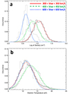 |
Fig. A.1. Histograms of (a) the logarithm of the electron density and (b) the electron temperature for three different bins of solar wind speed Vsw. The colored lines represents Gaussian fits to the observed distributions. |
Statistics of parameters presented in Figure 8.
Statistics of parameters presented in Figure 9.
Statistics of core parameters presented in Figure 10.
Statistics of halo parameters presented in Figure 11.
Statistics of strahl parameters presented in Figure 12.
Statistics of density ratios presented in Figure 14.
Statistics of temperature ratios presented in Figure 15.
All Tables
All Figures
|
Fig. 1. Illustration of the three solar wind electron populations: the core, halo, and strahl. The top row shows a 2D view of the eVDFs of these three components, and the bottom row highlights each component in parallel cuts through the eVDFs. |
| In the text | |
|
Fig. 2. Example of a typical voltage power spectrum around the electron plasma frequency measured by the Wind/WAVES/TNR instrument in the solar wind on June 25, 1995. The solid line is the predicted spectrum fitted to the selected data (in diamonds) among data not retained (dots) for the QTN fitting (see text). The annotations indicate the electron parameters obtained by fitting the theoretical spectrum from the ion and the electron QTN, using a sum of two isotropic Mxwellians – a core “c” and a halo “h” – to the observed spectrum. The vertical line indicate the locations of the local electron plasma frequency obtained by both a Neural Network (“NN”, solid line) and by QTN fit (“fitted”, dashed line). |
| In the text | |
|
Fig. 3. Illustration of the iterative method for determining s/c potential (see text for details). We arrive at an estimated value ϕ of the s/c potential by iterating through various “candidate” s/c potentials, minimizing the difference between the electron density determined as the first-order moment of the eVDF and the electron density obtained from the QTN method. |
| In the text | |
|
Fig. 4. Two typical eVDFs measured by EESA-L and EESA-H at 1 au in the slow solar wind – panels (a) and (c) –, and in the fast solar wind – panels (b) and (d). The top panels (a) and (b) show cuts through the eVDF in one of the two directions perpendicular to the local magnetic field B: the diamonds are data points from EESA-L and the asterisks from EESA-H. The dotted lines represent the one-count levels for EESA-L and EESA-H. The blue dashed line represents the sum of Maxwellian and κ-distributions calculated using the QTN fit parameters (indicated in blue), which are used to initialize the eVDF fit. The red line represents the fit to the measured perpendicular eVDF cut; the resulting fit parameters are indicated in red. The bottom panels (c) and (d) show cuts through the eVDF in the direction parallel to B. The perpendicular fit is reported in red, and the perpendicular fit parameters are used to initialize the parallel eVDF fit, the results of which are given in green. In each plot, the points that are selected for inclusion in the eVDF fit are filled with pink color. |
| In the text | |
|
Fig. 5. Illustration of the algorithm used to extract the strahl from the eVDFs of Fig. 4; the left panel (a) shows the slow wind eVDF and the right panel (b) shows the fast wind eVDF. Cuts through the Δ distribution (see text) in the parallel and perpendicular direction are indicated in red and blue, respectively. The obvious peak in the parallel cut in red shows the range and structure of the strahl. In the fast wind, the strahl is much more prominent than in the slow wind. However, the strahl is wider in the slow wind than in the fast wind. The dashed horizontal line represents the threshold for the automated extraction of the strahl. |
| In the text | |
|
Fig. 6. 2D distribution of the strahl after extraction from the total observed eVDF. The left panel (a) and the right panel (b) are the same slow and fast solar wind examples as in Figs. 4 and 5. The calculated strahl moments for each example are listed. |
| In the text | |
|
Fig. 7. Probability distributions of the solar wind speed Vsw. The black histogram represents the distribution based on our eVDF analysis, and the red histogram represents the distribution based on 3DP onboard proton moments, normalized to the maximum of the eVDF historgram. |
| In the text | |
|
Fig. 8. Column-normalized 2D histrograms of parameters of the total electron species: (a) electron density Ne, (b) total electron temperature Te, (c) temperature Te∥ of the total electron distribution in the direction parallel to the mean magnetic field, (d) temperature Te⊥ of the total electron distribution in the direction perpendicular to the mean magnetic field, (e) temperature ratio Te⊥/Te∥ of the total electron distribution, and (f) magnitude of the parallel heat flux |Qe∥| of the total electron distribution. |
| In the text | |
|
Fig. 9. Column-normalized 2D histrograms of proton parameters and derived total electron parameters: (a) total proton temperature Tp, (b) temperature ratio Te/Tp of the total proton and electron distributions, (c) βp of the total proton distribution, and (d) βe of the total electron distribution. |
| In the text | |
|
Fig. 10. Column-normalized 2D histrograms of electron core parameters: (a) core density Nc, (b) sign-corrected drift speed Vdc sign(Qe∥) between core and proton bulk velocity, (c) temperature Tc∥ of the core in the direction parallel to the mean magnetic field, (d) temperature Tc⊥ of the core in the direction perpendicular to the mean magnetic field, (e) total temperature Tc of the core, and (f) temperature ratio T⊥/T∥ of the core. |
| In the text | |
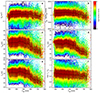 |
Fig. 11. Same as Fig. 10, but for the halo instead of the core. |
| In the text | |
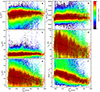 |
Fig. 12. Same as Fig. 10, but for the strahl instead of the core. |
| In the text | |
|
Fig. 13. Current balance of the total electron distribution function. |
| In the text | |
|
Fig. 14. Density ratios of the electron components as functions of Vsw. (a) Nh/Nc, (b) Ns/Nc, and (c) Ns/Nh. |
| In the text | |
|
Fig. 15. Ratios of the scalar temperatures of the electron components as functions of Vsw. (a) Th/Tc, (b) Ts/Tc, and (c) Ts/Th. |
| In the text | |
|
Fig. 16. Intercorrelations between electron temperature ratios and density ratios. (a) Th/Ts as a function of Nh/Nc, (b) Ts/Tc as a function of Ns/Nc, and (c) Ts/Th as a function of Ns/Nh. |
| In the text | |
|
Fig. A.1. Histograms of (a) the logarithm of the electron density and (b) the electron temperature for three different bins of solar wind speed Vsw. The colored lines represents Gaussian fits to the observed distributions. |
| In the text | |
Current usage metrics show cumulative count of Article Views (full-text article views including HTML views, PDF and ePub downloads, according to the available data) and Abstracts Views on Vision4Press platform.
Data correspond to usage on the plateform after 2015. The current usage metrics is available 48-96 hours after online publication and is updated daily on week days.
Initial download of the metrics may take a while.