| Issue |
A&A
Volume 674, June 2023
|
|
|---|---|---|
| Article Number | A74 | |
| Number of page(s) | 7 | |
| Section | Stellar atmospheres | |
| DOI | https://doi.org/10.1051/0004-6361/202346125 | |
| Published online | 06 June 2023 | |
Secrets behind the RXTE/ASM light curve of Cyg X-3
Feedback between wind-fed accretion and luminosity
1
Dept of Physics,
PO Box 84,
00014 University of Helsinki,
Finland
e-mail: This email address is being protected from spambots. You need JavaScript enabled to view it.
2
Institutt for Fysikk, Norwegian University of Science and Technology,
Högskoleringen 5,
Trondheim
7491, Norway
e-mail: This email address is being protected from spambots. You need JavaScript enabled to view it.
3
Sky & Telescope,
1374 Massachusetts Ave Floor 4,
Cambridge, MA
02138, USA
e-mail: This email address is being protected from spambots. You need JavaScript enabled to view it.
Received:
11
February
2023
Accepted:
31
March
2023
Abstract
Context. In wind-fed X-ray binaries, the radiatively driven wind of the primary star can be suppressed by the X-ray irradiation of the compact secondary star, leading to an increased accretion rate. This causes feedback between the released accretion power and the luminosity of the compact star (X-ray source).
Aims. We investigate the feedback process between the released accretion power and the X-ray luminosity of the compact star (a low-mass black hole) in the unique high-mass X-ray binary Cygnus X-3. We study whether the seemingly erratic behavior of the observed X-ray light curve and accompanying spectral state transitions could be explained by this scenario.
Methods. The wind-fed accretion power is positively correlated with the extreme-ultraviolet (EUV) irradiation of the X-ray source. It is also larger than the bolometric luminosity of the X-ray source derived by spectral modeling and assumed to be an intrinsic property of the source. We assume that a part of the wind-fed power experiences a small amplitude variability around the source luminosity. The largest luminosity (lowest wind velocity) is constrained by the Roche-lobe radius, and the lowest one is constrained by the accretion without EUV irradiation. There is a delay between the EUV flux fixing the wind-fed power and that from the source. We modeled this feedback assuming different time profiles for the small amplitude variability.
Results. We propose a simple heuristic model to couple the influence of EUV irradiation on the stellar wind (from the Wolf-Rayet companion star) with the X-ray source itself. The resulting time profile of luminosity mimics that of the input variability, albeit with a larger amplitude. The most important property of the input variability are turnover times when it changes its sign and starts to have either positive or negative feedback. The bolometric luminosity derived by spectral modeling is the time average of the resulting feedback luminosity.
Conclusions. We demonstrate that the erratic behavior of the X-ray light curve of Cygnus X-3 may have its origin in the small amplitude variability of the X-ray source and feedback with the companion wind. This variability could arise in the accretion flow and/or due to the loss of kinetic energy in a jet or an accretion disk wind. In order to produce similar properties of the simulated light curve as observed, we have to restrict the largest accretion radius to a changing level, and assume variable timescales for the rise and decline phases of the light curve.
Key words: stars: individual: Cyg X-3 / binaries: close / stars: black holes / X-rays: individuals: Cyg X-3
© The Authors 2023
 Open Access article, published by EDP Sciences, under the terms of the Creative Commons Attribution License (https://creativecommons.org/licenses/by/4.0), which permits unrestricted use, distribution, and reproduction in any medium, provided the original work is properly cited.
This article is published in open access under the Subscribe to Open model. This email address is being protected from spambots. You need JavaScript enabled to view it. to support open access publication.
1 Introduction
Cygnus X-3 (4U 2030+40), one of the first X-ray binaries discovered (Giacconi et al. 1967), is also one of the brightest in the X-ray and radio regimes. It is listed in the catalogue of High-Mass X-ray Binaries (HMXB) in the Galaxy (Liu et al. 2006b), where most entries consist of an OB star whose wind feeds a companion neutron star or black hole, releasing X-rays in the process. The donor star of Cyg X-3 (optical counterpart V1521 Cyg) is a Wolf-Rayet (WR) star either of type WN 5-7 (van Keerkwijk et al. 1996) or a weak-lined WN 4-6 (Koljonen & Maccarone 2017). The relatively small size of this helium star allows for a tight orbit with a period of 4.8 h which is more typical of low-mass X-ray binaries. Cyg X-3 is often classified as a microquasar and the radio, infrared, and X-ray properties suggest that the companion star is a low-mass black hole, although a neutron star cannot be totally ruled out (Zdziarski et al. 2013).
Vilhu et al. (2021) show quantitatively how the wind velocity of the WR star on the face-on side depends on the extreme-ultraviolet (EUV) irradiation (at 100 eV) from the compact star, in agreement with the results by Krticka et al. (2018) for irradiation effects in HMXBs. Increasing the EUV leads to the suppression of wind velocity. This, in turn, increases the accretion rate and released accretion power due to the more effective wind capture rate of the compact star. Therefore, there exists a positive correlation between the EUV irradiation and the power provided by the wind accretion.
A similar correlation exists between the EUV flux and the bolometric luminosity Lbol (= Leqpair) released by the X-ray source itself as demonstrated by Hjalmarsdotter et al. (2009) using the hybrid thermal and nonthermal plasma emission model EQPAIR (Coppi 1992). The variability of the EUV irradiation leading to changes in the wind velocity and subsequently the wind-fed accretion luminosity may be behind the evolution of the X-ray RXTE/ASM light curve of CygX-31.
A part of the wind-fed power goes to the observed radiation of the X-ray source (Lrad), while a part is advected to the black hole and/or lost from the system by jets or accretion disk winds. In the present paper, we propose a heuristic model by balancing between Lrad and Leqpair. These should be equal but we assume a small variability around this equality; Leqpair is a time average of Lrad and characteristic of the X-ray source.
2 Methods
Hjalmarsdotter et al. (2009) analyzed an extensive set of RXTE spectra of Cyg X-3 and fitted them with EQPAIR spectral modeling by Coppi (1992) during five spectral states (see Fig. 1). The bolometric luminosities Lbol (= Leqpair) of these states are plotted in Fig. 2 versus the EUV flux (EFE at 100 eV) at the system using a distance of 7.4 kpc (McCollough et al. 2016) and correcting the fluxes given in Vilhu et al. (2021) to this distance (dashed line). The system is optically too weak for a Gaia distance estimate (due to strong absorption). We also corrected the fluxes for orbital modulation using the observing log in Hjalmarsdotter et al. (2009), estimating the modulation between 2 and 100 keV from Vilhu et al. (2003; see their Fig. 3 and the folding ephemeris there). This amounted to a correction factor 1.3–1.4. The fluxes are given in Table 1.
For comparison, the wind-fed accretion power Pacc is shown in Fig. 2 (solid line) as computed from the Bondi-Hoyle-Lyttleton (BHL) formalism using a wind model with clumping volume filling factor 0.1 (see Eqs. (2)–(5) and Table 1). Clumpy winds are ubiquitous in hot stars. The value 0.1 means that all the wind mass in clumps comprises 10% of the total wind volume. On average, the wind-fed accretion power is a factor of 2 larger than the bolometric luminosity likely arising from the power lost in the advective and/or kinetic components (vertical line in Fig. 2). The wind-fed power without the effect of EUV irradiation would result in 1.35 × 1038 erg s−1 (horizontal line in Fig. 2).
We adopted masses of 2.4 M⊙ and 10 M⊙ for the compact star and WR star, respectively, and the wind mass-loss rate Ṁwind = 6.5 × 10⁻⁶ M⊙ year−1 used in Vilhu et al. (2021). These all are mean values within error bars given by Zdziarski et al. (2013). Their solution allows for the presence of either a neutron star or a low-mass black hole, but they consider that the radio, infrared, and X-ray properties of the system suggest that the compact star is a black hole. In the present paper, we adopt this view.
Wind models were computed with the methods explained in Vilhu et al. (2021), integrating the mass conservation and momentum balance equations with the upward booster (line force). The computation of the line force is explained in Appendix B of Vilhu et al. (2021) utilizing the XSTAR data-base2.
In the modeling we used a wind clumping volume filling factor fvol = 0.1 similar to that in Vilhu et al. (2021; Table A.1, mean of phase angles 0° and 30°), except that the nonirradiated model (NOX) has the velocity at infinity Vinf = 1600 km s−1 (as in WNE-w stars, Hamann et al. 1995, their Fig. 3). For the different spectral states (no EUV irradiation, NOX; hard, HARD; soft nonthermal, SNTH; intermediate, INT; ultra soft, US; and very high, VH), the EUV fluxes, bolometric luminosities, and wind velocities at a compact star distance (without gravitational pull) are given in Table 1. Examples of the wind simulations are shown in Fig. 3.
To guarantee convergence, it is essential to use a reliable fitting model. We used the β-velocity model (V = Vinf (1 − Rstar/r)β) but multiplied it by a suppression factor SF. In this way the model mimics the bowed (due to EUV irradiation) velocity curves of Fig. 3 below the kinks, and SF can be written as
 (1)
(1)
where a and b are the fitting parameters and x = r/Rstar is the distance from the WR surface (x =1 and 3.4 at the surface and CS distance, respectively). The fitting with the model was performed when the velocity gradient was large enough to provide a positive line force (left from the kinks in the curves of Fig. 3). When the gradient became small, the force vanished (strongly depending on the velocity gradient), and the velocity and density values at the kink determined the wind particle flying outward. Vilhu et al. (2021) used another form of SF above the kink, but we consider the present approach better. One could in principle combine these two suppression factors providing too many free parameters.
In the BHL formalism, the accretion radius is
 (2)
(2)
where the relative velocity Vrel was computed from the wind velocity at the compact star location and the orbital velocity of the compact star as
 (3)
(3)
where Vorb = 675 km s−1 for the masses used. The gravitational pull of the compact star is not included because it is taken into account in the BHL formalism itself.
The wind-fed accretion power was then computed from
 (4)
(4)
where the mass accretion rate is
 (5)
(5)
where A is the binary separation (3.4 R⊙), Mwind is the mass-loss rate of the WR star, and the mass-to-energy conversion factor η = 0.1 is approximately valid for neutron stars and black holes (Frank & Raine 1992).
We assume that a part of the wind-fed power Pacc goes to the radiation luminosity Lrad of the X-ray source, and a part of it goes to advection Ladv (negative) and kinetic energy of the jets and accretion disk wind Lkin (Narayan & Yi 1994; notation from Fender & Munoz-Darias 2016):
 (6)
(6)
The bolometric radiation luminosity of the source Leqpair (derived from EQPAIR modeling) is the intrinsic property of the X-ray source and is equal to Lrad,
 (7)
(7)
but we assume a small variability ϵ in this equality. Either Leqpair or Lrad vary, or both of them do. When Lrad is responsible for ϵ (Leqpair being constant), this means, for example, that advection changes with time, and the physics of which depends on the flow (see e.g., Esin et al. 1997; Liu et al. 2006a; Cao 2016). In this case, Leqpair(EUV) is a time average of Lrad(EUV). When discussing masses, Vilhu et al. (2021) assumed that all wind-fed power goes to radiation. This, however, did not influence their wind modeling.
Figure 4 gives the basic idea of the present study, in the case when Leqpair(EUV) is constant and Lrad(EUV) is varied by ϵ(time). The results are identical if Leqpair is variable. The only difference is that the evolution in Fig. 4 goes counterclockwise (UP and DOWN change place). The solid line is Leqpair around which the dashed lines, representing Lrad, vary at the ϵ distance. In the plot two ϵ values are shown (+0.5 and −0.5). There is a delay between EUV fluxes from wind-fed power and that from the source. We modeled this feedback using the viscosity timescales at the circularization radius and timescales from the ASM light curve, and assuming different time profiles for ϵ.
At point 1 (Fig. 4, right panel), the radiation luminosity Lrad was determined from the wind with EUV flux there. The source finds a state corresponding to this luminosity which, in turn, determines the EUV flux (at point 2) and corresponding wind velocity and accretion luminosity (point 3). In this way the process continues upward (positive feedback). In the case in which ϵ is negative, the process goes downward (points 4-5-6, negative feedback). We assume that the output luminosity comes from Lrad and Leqpair is its time average. A fraction of the wind-fed power Pacc goes to kinetic energy and advection (see Fig. 2).
We set the viscosity time at the circularization radius for the duration of one step in the upward and downward channels (1-2-3 or 4-5-6). One step corresponds, on average, to a luminosity change around 1037 erg s−1. This choice determines how steep the rises and declines are. In numerical simulations of Sect. 3, other choices are also presented. The time spent in high and low states is determined by the time profile of ϵ. At EUV fluxes 0.25 and 1.26 (hard and very high states), these viscosity times are 1.1 and 4.1 days, respectively, as computed from the formula given in CAO & Zdziarski (2020):
 (8)
(8)
where tvisc is in days, R is the distance from the compact star, and RL is its Roche-lobe radius computed from the standard formula
 (9)
(9)
where A is the binary separation and q is the mass ratio Mcs/Mwr For the masses used, RL = O.88R⊙. We assume that μ = 4/3 (the mean molecular weight of fully ionized Helium gas), Τ = 105 Κ (radiation black-body temperature of the WR star), and α = 0.1 (viscosity parameter).
The circularization radius was computed from (see e.g., Kretschmar et al. 2021)
 (10)
(10)
The upward process continues until the accretion radius Racc is close to the Roche-lobe radius RL or else the increasing EUV flux combined with the decrease in clumping stops the wind, and the process starts again. In Fig. 4 (left), the maximum value is marked (see the oval “O” in the upper right corner). One can also speculate that changing the filling factor from 0.1 (the baseline value) to 0.3 may lead to the cessation of the wind during the very high state (see Fig. 3). This influences the highest luminosity reached.
In our simulations (next section), we used the 0.9 × RL limit for the maximum accretion radius, which gave a maximum luminosity of 5.3 × 1038 erg s−1 (a bit less than the Eddington luminosity for ionized helium). This limit was a random choice, but we followed the reasoning from CAO & Zdziarski (2020) that the accretion disk is tidally limited by 0.9 × RL. We assumed the same for the accretion radius. The system stays at a high level unless the channel down opens (ϵ becomes negative, starting negative feedback). The oval “O” in the lower-left corner of Fig. 4 (left) shows the lowest level where the system ends after the downward motion. In our simulations it was set to the NOX accretion power value 1.35 × 1038 erg s−1. When the upward channel opens (ϵ becomes positive, positive feedback), a new climb upward starts. In the next section, we illustrate this process by model computations and propose the origin for the ASM light-curve variability.
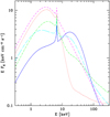 |
Fig. 1 Unabsorbed model spectra of the five main spectral states of Cyg X-3 reproduced from Hjalmarsdotter et al. (2009). The models corresponding to the hard state (solid blue line), the intermediate state (long-dashed cyan line), the very high state (short-dashed magenta line), the soft nonthermal state (dot-dashed green line), and the ultrasoft state (dotted red line) are shown (unabsorbed at Earth). |
EUV fluxes (EUV = EFE in units of 2 × 1036 erg s−1 at 100 eV), model luminosities (Lbol = Leqpair 1038 erg s−1), and wind velocities (Vwind km s−1) without the gravitational pull of the compact star at its distance on the face-on side and wind-fed accretion power Pacc (1038 erg s−1) for the spectral states used.
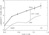 |
Fig. 2 Wind-fed power Pacc of Cyg X-3 as a function of the EUV irradiation (EFE in units of 2 × 1036 erg s−1 at 100 eV) as computed with the Bondi-Lyttleton formalism (solid line with error bars) from the wind velocities of Table 1. A similar relation for the bolometric luminosity Leqpair = Lbol of the X-ray source itself is shown by the dashed line, and it was obtained by EQPAIR modeling of X-ray spectra (Hjalmarsdotter et al. 2009). The horizontal line shows the power provided by the wind without EUV irradiation (NOX). The positions of the hard and very high spectral states are marked (HARD and VH). The vertical line shows the amount of power going to kinetic and advective parts. |
 |
Fig. 3 Wind velocity models of the WR component at the face-on side are plotted versus distance from the WR surface. The models were computed without the gravitational pull of the compact star (the distance of which is marked by CS). The numbers 0.1 and 0.3 along the curves mean clumping volume filling factors fvol. The labels HARD and VH mean the wind during the hard and very high states, respectively; and 2*VH means doubling of the very high state EUV flux. The kinks (discontinuities) are due to stopping the line force. |
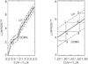 |
Fig. 4 Basic idea of the present paper. Left panel: bolometric X-ray source luminosity Leqpair (in units of 1038 erg s−1) of Fig. 2 is shown versus the EUV irradiation from the X-ray source (EFE in units of 2 × 1036 erg s−1 at 100 eV; solid line). Around it, Lrad is variable and two positions are shown (dashed lines). When Lrad − Leqpair = ϵ is positive, the evolution goes upward, “UP” (1-2-3, positive feedback), when negative it goes downward, “DOWN” (4-5-6, negative feedback). Right panel: zoomed version of the panel on the left. |
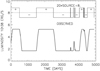 |
Fig. 5 Upper part of the plot: randomly selected box-like time profile for ϵ (=SOURCE, in the plot multiplied by 20). Lower plot: observed luminosity after the feedback steps outlined in Sect. 2. The plus and minus signs in the upper plot mark the times of positive and negative feedback, respectively (ϵ positive or negative). See text for details. |
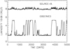 |
Fig. 6 Upper plot: assumed ϵ profile in Eq. (7) resembling the ASM daily light curve (=SOURCE). Lower plot: observed luminosity after the feedback process outlined in Sect. 2. See text for details. |
3 Numerical results
We show numerical simulations based on the previous section, assuming that Lrad is variable using two types of time profiles for ϵ (in Eq. (7)): (i) a random box-style profile and (ii) a profile that mimics the ASM daily light curve.
3.1 Box profile
We made a random box-like ϵ profile, which is shown in the upper part of Fig. 5. Boxes were selected to show the effect of different timescales during low and high states. The profile is symmetrical around zero mean. The amplitude of the profile is not very constraining and could have been either smaller or larger, resulting in a similar observed luminosity after the feedback steps (Fig. 5 bottom). The rise and decline parts are slightly tilted due to the viscosity timescales used (1.1 and 4.1 days at hard and very high state levels, respectively) for one step with ann average luminosity change of 1037 erg s−1. Timescales for other phases were linearly interpolated from these two values.
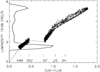 |
Fig. 7 Luminosity (in units of ΙΟ38 erg s−1) plotted against the EUV flux (EFE in units of 2 × 1036 erg s−1 at 100 eV) for the simulation of Sect. 3.2 shown in Fig. 6. The mean location of spectral states are marked as follows: HAR = hard, SNT = soft nonthermal, INT = intermediate, US = ultrasoft, and VH = very high. The histogram on the left (thick solid line) shows the relative number of days spent at fixed luminosity. The dashed line shows Leqpair. |
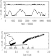 |
Fig. 8 Same as Fig. 6 (upper panel) and Fig. 7 (lower panel), but with 4 times longer rise and decline times in the light curve. |
3.2 ASM profile
In the simulation, the time profile of ϵ was taken directly from the observed ASM daily light curve by ϵ = O.O2×(ASM counts s−1 −15; the upper part of Fig. 6). The normalization of ϵ is ad hoc. However, the results are not very sensitive to the amplitude of ϵ. The profile is rather symmetrical around zero, but shifting the zero level lower would not change the results significantly.
The essential property of the ϵ time profile are turnovers of its sign (changing to positive or negative feedback).
Using the selected expression for ϵ basically means picking turnover times from the ASM daily light curve at 15 counts s−1 level. The rise and decline times used for one step with an average luminosity change of 1037 erg s−1 were the viscosity timescales at circularization radii (1.1 and 4.1 days at hard and very high state levels, respectively). The lower part of Fig. 6 shows the resulting light curve explained in Sect. 2. As expected, this light curve is qualitatively very similar to the ϵ time profile (upper plot) reflecting its turnover times.
Figure 7 shows the evolution of the light curve in the EUV-L diagram. Luminosity (in units of 1038 erg s−1) is plotted against the EUV flux (EFE in units of 2 × 1036 erg s−1 at 100 eV) for the simulation shown in Fig. 6. The mean location of spectral states are marked. The dashed line shows Leqpair. The histogram on the left (thick solid line) shows the relative number of time spent at fixed luminosity.
Figure 8 shows the effect of lengthening the rise and decline times by a factor of 4 from those used in Figs. 6 and 7. This smooths the light curve and the luminosity histogram.
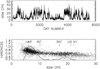 |
Fig. 9 Upper panel: RXTE/ASM daily light curve of Cyg X-3. Lower panel: Hardness [C−A]/[C+A] versus count rate (dots). The solid line shows the histogram (relative number of days/ASM bin). The mean positions of spectral states are marked as follows: HAR = hard, SNT = soft nonthermal, INT = intermediate, US = ultrasoſt, and VH = very high. |
4 Observed ASM histogram
In the previous section, luminosity histograms were shown for the simulated light curves (see Figs. 7 and 8, lower plot). We present a similar histogram for the ASM light curve to be compared.
A partial gap between low and high states exists in the observed ASM light curve, which is illustrated in Fig. 9 (lower panel), where the hardness [(C−A)/(C+A)] is plotted against the daily mean count rate. The energy range of ASM is 1.5–12.1 keV with filters A (1.5–3 keV) and C (5–12.1 keV). The solid line in the lower plot shows the histogram of the relative number of days spent in the ASM daily count rate bin (1 ct s−1). Mean count rates of the spectral states are marked as estimated from the observing log of Hjalmarsdotter et al. (2009). We note that the places of the intermediate and soft nonthermal states are reversed in Figs. 7 and 9. This is due to their different spectral shapes (see Fig. 1).
Comparing the simulated histograms of Sect. 3.2 with the observed ASM histogram (Fig. 9, lower panel), we suggest a variable maximum accretion radius (in simulations set to 0.9 × RL) and/or variable timescales of rise and decline phases of the light curve. Both of these smear the histogram closer to that of ASM.
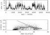 |
Fig. 10 Upper panel: RXTE/ASM daily light curve of Cyg X-3 (the dotted line) overplotted with the smoothed version used for timescale estimates (the solid thick line). Lower panel: mean daily changes (counts s−1, the solid thick line) with error bars. Dots give individual daily changes. The solid linear line gives a comparison with the timescales used in Sect. 3 (see the text). |
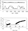 |
Fig. 11 Results of simulations with timescale estimates from smoothed ASM light curve (see Fig. 10 and text). Upper panel: same as Fig. 6. Lower panel: same as Fig. 7. |
5 Timescales from the ASM light curve
The timescale estimate used during the rising and declining parts of the light curve was crude (1.1 and 4.1 days during the hard and very high state, respectively). We compare it with that derived from the ASM light curve itself.
We built a smoothed version of the daily ASM light curve shown in Fig. 10 (upper panel, solid line). The original light curve is shown by the dotted line. The smoothing was done by a box car with a 60 days width. From this smoothed light curve, mean differences (absolute values) between subsequent days were determined at binned ASM count rate intervals and their standard deviations were computed. This is shown in Fig. 10 (lower panel). The dots show individual changes during one day, while the solid thick line gives the mean value with one-sigma errors.
Assuming that the luminosity L (in units of 1038 erg s−1) can be approximated by the ASM count rate divided by six, and that the feedback step is around 1037 erg s−1, we can mark the timescales of our simulations in Fig. 10 (lower panel, the solid linear line). The approximate factor 6 comes from comparisons of ASM count rates with EQPAIR luminosities.
The timescale for the feedback steps can be computed as follows. Marking the mean value of the daily change by YASM (Fig. 10 lower panel, thick solid line with error bars), then the time spent for one step is DL/(YASM/6) where DL is the luminosity change during one step (in units of 1038 erg s−1). Using this timescale, we repeated the computations performed in Sect. 3. The results are shown in Fig. 11. These results are between those in Sect. 3.2 using tvisc and 4tvisc. Due to the scaling used (the factor 6), the maximum luminosity level is also lower.
6 Discussion
Without EUV irradiation of the X-ray source, it is impossible to provide enough power for all spectral states (see Fig. 2), provided that the mass of the compact star and mass-loss rate of the WR star are not higher than what is assumed in the present paper (2.4 Μ⊙ and 0.65 × 10⁻⁵ M⊙ yr−1). As an example, the combination of 3.5 M⊙ and 1.0 × 10⁻⁵ M⊙ yr−1 would give enough accretion power for all spectral states by the pure wind model without EUV irradiation (see Fig. 2, the horizontal NOX line would rise threefold). These parameter values are within acceptable ranges. However, even in this case, the wind-fed power has a positive correlation with the EUV flux and the process outlined here should work.
We have proposed a heuristic feedback model to relate the X-ray variability of Cyg X-3 to the X-ray irradiation on the face-on side of the WR companion, and subsequent lowering of the wind velocity and increasing wind-fed accretion. The Bondi-Lyttleton-Hoyle modeling used to estimate the wind-fed power (Eq. (4)) is approximate and very sensitive to the wind velocity. For our purposes, the plot in Fig. 2 demonstrates that the wind-fed power is larger than what the source radiates. In the present work, we have assumed that a part of it goes to radiation (Lrad), which is varying by a small factor ϵ (Eq. (7)). In the model a small seed ϵ can produce the ASM light curve, although the process works for different amplitudes of ϵ. The size of ϵ is not crucial with the essential property being turnover times when ϵ changes its sign and starts positive or negative feedback.
The kink in Leqpair around EUV flux = 0.7 (see Figs. 2 and 7) may have some meaning, but it is not crucial here because identical results can be observed by straightening the kink. The kink is caused by the nonlinear behavior of Leqpair around the soft nonthermal and intermediate states (see Fig. 1) and should be confirmed. The main reason for the kink seems to be the intermediate state spectral model (Fig. 1). The intermediate state refers to a transitional spectral state between the hard and soft states. The low ASM count rate of the intermediate state (Fig. 9) supports the kink and low bolometric luminosity.
We approximated the physics involved by an ad hoc scaling law type process. The ends of the high and low states (ovals “O” in Fig. 4) were set by the Roche-lobe and NOX limits, respectively. Their durations, in turn, are due to opening of the upward and downward channels (turnover times of ϵ). We have assumed that this process takes place in steps between the baseline Leqpair, characterizing the X-ray source, and a small deviation from it (Leqpair ± ϵ). The real physics of this process remains to be clarified, but first steps could be done as follows. A simple case would be when the advective and kinetic parts in Eq. (6) were zero: Pacc = Lrad. Then the feedback process could be done without injecting ϵ into Eq. (7). If the X-ray source model was simple as in an accretion disk, one should be able to directly follow the feedback process without ϵ, provided one has access to a physical time-dependent accretion disk code. Further, if the advective and kinetic parts were not zero, one could repeat this as outlined in the present paper and compare the results.
In each upward and downward step, the EUV flux changes, affecting the wind velocity and mass accretion rate. We assumed that the wind relaxation takes place more rapidly (in less than hours) than the viscosity timescale of the disk at a circularization radius (days). Wind particles travel across the wind in less than half an hour (Vilhu et al. 2021) and thermal timescales are very small because the wind mass is small (on the order of 10−9M⊙).
Variations in ϵ can be caused by variable kinetic energy (jets, accretion disk wind) and/or advection, the physics of which are not fully understood (see e.g., Esin et al. 1997; Liu et al. 2006a; Cao 2016). To explain the smooth distribution of ASM count rates (the histogram in Fig. 9, lower panel), one has to assume either a variable maximum accretion radius and/or changing timescales during the rise and decline parts of the light curve. The effects of these are illustrated by histograms in Figs. 7, 8, and 11, and clearly need further work.
Many wind-fed X-ray binaries are expected to experience a qualitatively similar behavior, for example Cyg X-1, which is a very tight system with a binary separation about twice the OB-supergiant radius. For comparison, in Cyg X-3 the separation is 3.4 times the WR-star radius.
7 Conclusions
We propose a simple heuristic model to investigate the feedback between the WR wind and the X-ray source of Cyg X-3. In our model, the radiation from accretion Lrad fluctuates around the mean value Leqpair characteristic of the X-ray source and derived from modeling time-averaged X-ray spectra. There is a delay between EUV fluxes determining the wind-fed power and the bolometric luminosity.
We modeled this feedback using viscosity timescales and assumed different time profiles for variability (ϵ in Eq. (7)). More realistic timescales were estimated from the smoothed ASM light curve (Sect. 5). These timescales determine the rise and decline times of the light curve, while the ϵ time profile sets limits on the duration of low and high states. The essential property of ϵ are turnover times when it changes sign and starts positive or negative feedback.
We have demonstrated how light-curve variations of Cyg X-3 can have their origin in small temporal changes of the accretion flow (ϵ in Eq. (7)). These changes may be variations in advection and/or kinetic energy (jets, accretion disk wind). The time profile of the resulting luminosity mimics the input ϵ but it is magnified (see Figs. 5 and 6). Comparing the histograms of Figs 7–9, and 11, additional variable parameters (besides ϵ) are needed. We suggest a variable maximum accretion radius and/or changing timescales for the rise and decline parts of the light curve.
Acknowledgements
This project has received funding from the European Research Council (ERC) under the European Union’s Horizon 2020 research and innovation programme (grant agreement No. 101002352). We thank Dr Linnea Hjalmarsdotter for permission to use her Fig. 1.
Note added in proof Table 1 has been updated during the production process. The current Table 1 gives the correct values.
References
- Cao, X. 2016, ApJ, 817, 71 [NASA ADS] [CrossRef] [Google Scholar]
- Cao, X., & Zdziarski, A. A. 2020, MNRAS, 492, 223 [NASA ADS] [CrossRef] [Google Scholar]
- Coppi, P. 1992, MNRAS, 258, 657 [Google Scholar]
- Dubus, G., Cerutti, B., & Henri, G. 2010, MNRAS, 404, L55 [NASA ADS] [Google Scholar]
- Esin, A. A., McClintock, J.E., & Narayan, R. 1997, ApJ, 489, 865 [NASA ADS] [CrossRef] [Google Scholar]
- Fender, R., & Munoz-Darias, T. 2016, Lecture Notes Phys., 905, 65 [NASA ADS] [CrossRef] [Google Scholar]
- Frank, J., King, A., & Raine, D. 1992, Accretion Power in Astrophysics, Cambridge Astrophysics Series 21, 2nd edn. (Cambridge: Cambridge University Press), 4 [Google Scholar]
- Giacconi, R., Gorenstein, P., Gursky, H., & Waters, J. P. 1967, ApJ, 148, L119 [NASA ADS] [CrossRef] [Google Scholar]
- Hamann, W.-R., Koesterke, L., & Wessolowski, U. 1995, A&A, 299, 151 [NASA ADS] [Google Scholar]
- Koljonen, K. I. I., & Maccarone, T. J. 2017, MNRAS, 472, 78K [Google Scholar]
- Kretschmar, P., El Mellah, I., Martinez-Nunez, S., et al. 2021, A&A, 652, A95 [NASA ADS] [CrossRef] [EDP Sciences] [Google Scholar]
- Krticka, J., Kubat, J., & Krtickova, I. 2018, A&A, 620, A150 [NASA ADS] [CrossRef] [EDP Sciences] [Google Scholar]
- Liu, B. F., Meyer, F., & Meyer-Hofmeister, E. 2006a, A&A, 454, L9 [NASA ADS] [CrossRef] [EDP Sciences] [Google Scholar]
- Liu, Q. R., van Paradijs, J., & van den Heuvel, E. P. J. 2006b, A&A, 455, 1165 [NASA ADS] [CrossRef] [EDP Sciences] [Google Scholar]
- McCollough, M. L., Corrales, L., & Dunham, M. M. 2016, ApJ 830, L36 [NASA ADS] [CrossRef] [Google Scholar]
- Narayan, R., & Yi, I. 1994, ApJ, 428, L13 [Google Scholar]
- Hjalmarsdotter L., Zdziarski, A. A., Szostek, S., & Hannikainen, D. C. 2009, MNRAS, 392, 251 [NASA ADS] [CrossRef] [Google Scholar]
- van Keerkwijk, H. M., Geballe, T. R., King, D. L., van der Klis, M., & van Paradijs J. 1996, A&A, 314, 521 [NASA ADS] [Google Scholar]
- Vilhu, O., Hjalmarsdotter, L., Zdziarski, A. A. M. et al. 2003, A&A, 411, L405 [NASA ADS] [CrossRef] [EDP Sciences] [Google Scholar]
- Vilhu, O., Kallman, T. R., Koljonen, K. I. I., & Hannikainen, D. C. 2021, A&A, 649, A176 [NASA ADS] [CrossRef] [EDP Sciences] [Google Scholar]
- Zdziarski, A. A., Mikolajewska, J., & Belczynski, K. 2013, MNRAS 429, L104 [Google Scholar]
All Tables
EUV fluxes (EUV = EFE in units of 2 × 1036 erg s−1 at 100 eV), model luminosities (Lbol = Leqpair 1038 erg s−1), and wind velocities (Vwind km s−1) without the gravitational pull of the compact star at its distance on the face-on side and wind-fed accretion power Pacc (1038 erg s−1) for the spectral states used.
All Figures
|
Fig. 1 Unabsorbed model spectra of the five main spectral states of Cyg X-3 reproduced from Hjalmarsdotter et al. (2009). The models corresponding to the hard state (solid blue line), the intermediate state (long-dashed cyan line), the very high state (short-dashed magenta line), the soft nonthermal state (dot-dashed green line), and the ultrasoft state (dotted red line) are shown (unabsorbed at Earth). |
| In the text | |
|
Fig. 2 Wind-fed power Pacc of Cyg X-3 as a function of the EUV irradiation (EFE in units of 2 × 1036 erg s−1 at 100 eV) as computed with the Bondi-Lyttleton formalism (solid line with error bars) from the wind velocities of Table 1. A similar relation for the bolometric luminosity Leqpair = Lbol of the X-ray source itself is shown by the dashed line, and it was obtained by EQPAIR modeling of X-ray spectra (Hjalmarsdotter et al. 2009). The horizontal line shows the power provided by the wind without EUV irradiation (NOX). The positions of the hard and very high spectral states are marked (HARD and VH). The vertical line shows the amount of power going to kinetic and advective parts. |
| In the text | |
|
Fig. 3 Wind velocity models of the WR component at the face-on side are plotted versus distance from the WR surface. The models were computed without the gravitational pull of the compact star (the distance of which is marked by CS). The numbers 0.1 and 0.3 along the curves mean clumping volume filling factors fvol. The labels HARD and VH mean the wind during the hard and very high states, respectively; and 2*VH means doubling of the very high state EUV flux. The kinks (discontinuities) are due to stopping the line force. |
| In the text | |
|
Fig. 4 Basic idea of the present paper. Left panel: bolometric X-ray source luminosity Leqpair (in units of 1038 erg s−1) of Fig. 2 is shown versus the EUV irradiation from the X-ray source (EFE in units of 2 × 1036 erg s−1 at 100 eV; solid line). Around it, Lrad is variable and two positions are shown (dashed lines). When Lrad − Leqpair = ϵ is positive, the evolution goes upward, “UP” (1-2-3, positive feedback), when negative it goes downward, “DOWN” (4-5-6, negative feedback). Right panel: zoomed version of the panel on the left. |
| In the text | |
|
Fig. 5 Upper part of the plot: randomly selected box-like time profile for ϵ (=SOURCE, in the plot multiplied by 20). Lower plot: observed luminosity after the feedback steps outlined in Sect. 2. The plus and minus signs in the upper plot mark the times of positive and negative feedback, respectively (ϵ positive or negative). See text for details. |
| In the text | |
|
Fig. 6 Upper plot: assumed ϵ profile in Eq. (7) resembling the ASM daily light curve (=SOURCE). Lower plot: observed luminosity after the feedback process outlined in Sect. 2. See text for details. |
| In the text | |
|
Fig. 7 Luminosity (in units of ΙΟ38 erg s−1) plotted against the EUV flux (EFE in units of 2 × 1036 erg s−1 at 100 eV) for the simulation of Sect. 3.2 shown in Fig. 6. The mean location of spectral states are marked as follows: HAR = hard, SNT = soft nonthermal, INT = intermediate, US = ultrasoft, and VH = very high. The histogram on the left (thick solid line) shows the relative number of days spent at fixed luminosity. The dashed line shows Leqpair. |
| In the text | |
|
Fig. 8 Same as Fig. 6 (upper panel) and Fig. 7 (lower panel), but with 4 times longer rise and decline times in the light curve. |
| In the text | |
|
Fig. 9 Upper panel: RXTE/ASM daily light curve of Cyg X-3. Lower panel: Hardness [C−A]/[C+A] versus count rate (dots). The solid line shows the histogram (relative number of days/ASM bin). The mean positions of spectral states are marked as follows: HAR = hard, SNT = soft nonthermal, INT = intermediate, US = ultrasoſt, and VH = very high. |
| In the text | |
|
Fig. 10 Upper panel: RXTE/ASM daily light curve of Cyg X-3 (the dotted line) overplotted with the smoothed version used for timescale estimates (the solid thick line). Lower panel: mean daily changes (counts s−1, the solid thick line) with error bars. Dots give individual daily changes. The solid linear line gives a comparison with the timescales used in Sect. 3 (see the text). |
| In the text | |
|
Fig. 11 Results of simulations with timescale estimates from smoothed ASM light curve (see Fig. 10 and text). Upper panel: same as Fig. 6. Lower panel: same as Fig. 7. |
| In the text | |
Current usage metrics show cumulative count of Article Views (full-text article views including HTML views, PDF and ePub downloads, according to the available data) and Abstracts Views on Vision4Press platform.
Data correspond to usage on the plateform after 2015. The current usage metrics is available 48-96 hours after online publication and is updated daily on week days.
Initial download of the metrics may take a while.