| Issue |
A&A
Volume 674, June 2023
|
|
|---|---|---|
| Article Number | A83 | |
| Number of page(s) | 13 | |
| Section | Numerical methods and codes | |
| DOI | https://doi.org/10.1051/0004-6361/202345932 | |
| Published online | 06 June 2023 | |
A Gaussian process cross-correlation approach to time-delay estimation in active galactic nuclei★,★★
Astroinformatics, Heidelberg Institute for Theoretical Studies,
Schloss-Wolfsbrunnenweg 35,
69118
Heidelberg, Germany
e-mail: This email address is being protected from spambots. You need JavaScript enabled to view it.
Received:
18
January
2023
Accepted:
3
April
2023
Abstract
Context. We present a probabilistic cross-correlation approach to estimate time delays in the context of reverberation mapping (RM) of active galactic nuclei (AGN).
Aims. We reformulate the traditional interpolated cross-correlation method as a statistically principled model that delivers a posterior distribution for the delay.
Methods. The method employs Gaussian processes as a model for observed AGN light curves. We describe the mathematical formalism and demonstrate the new approach using both simulated light curves and available RM observations.
Results. The proposed method delivers a posterior distribution for the delay that accounts for observational noise and the non-uniform sampling of the light curves. This feature allows us to fully quantify the uncertainty on the delay and propagate it to subsequent calculations of dependant physical quantities, such as black hole masses. The method delivers out-of-sample predictions, which enables us to subject it to model selection, and can calculate the joint posterior delay for more than two light curves.
Conclusions. Because of the numerous advantages of our reformulation and the simplicity of its application, we anticipate that our method will find favour not only in the specialised community of RM, but also in all fields where cross-correlation analysis is performed. We provide the algorithms and examples of their application as part of our Julia GPCC package.
Key words: galaxies: active / quasars: general / galaxies: nuclei / galaxies: Seyfert / methods: statistical
The code can be downloaded from: https://github.com/HITS-AIN/GPCC.j1/. Also indexed under https://ascl.net/2303.006
Instructions and specific examples used in this paper can be found in: https://github.com/HITS-AIN/GPCCpaper
© The Authors 2023
 Open Access article, published by EDP Sciences, under the terms of the Creative Commons Attribution License (https://creativecommons.org/licenses/by/4.0), which permits unrestricted use, distribution, and reproduction in any medium, provided the original work is properly cited.
This article is published in open access under the Subscribe to Open model. This email address is being protected from spambots. You need JavaScript enabled to view it. to support open access publication.
1 Introduction
Reverberation mapping (RM; Cherepashchuk & Lyutyi 1973; Blandford & McKee 1982; Gaskell & Sparke 1986; Peterson et al. 2004) relies on observed variability to measure the time delay (τ) between changes in the continuum of the accretion disc (AD) and different regions in active galactic nuclei (AGN). In particular, the delay provides an estimate of the distance between AD continuum regions (or the AD size; RAD ∝ c • τAD, c is the speed of light; e.g. Pozo Nuñez et al. 2019; Cackett et al. 2020), between the broad emission line region (BLR) clouds and the AD (or the BLR size; RBLR ∝ c • τBLR, e.g. Grier et al. 2017; Kaspi et al. 2021), and between the AD continuum and the emission of a putative dust torus (or torus size; Rdust ∝ c • τdust, e.g. Landt et al. 2019; Almeyda et al. 2020). By combining spectro-scopic and photometric observations, the method has revealed black hole masses (MBH) and Eddington ratios in hundreds of AGN (see Cackett et al. 2021 and references therein).
Successful recovery of the time delay from an RM campaign depends on observational noise, intrinsic variability, and how well the light curves are sampled with respect to the delay. Highly sampled RM light curves may constrain the geometry of the reverberant region (e.g. Pancoast et al. 2012; Grier et al. 2013; Pozo Nuñez et al. 2014). However, astronomical observations are often affected by weather conditions, technical problems, sky coverage in the case of satellites, and seasonal gaps. Some of these effects are even more severe when observing high-redshift quasars. In this context, several algorithms have been proposed to deal with irregular time sampling. For example, traditional cross-correlation techniques applied to linearly interpolated data (ICCF; Gaskell & Peterson 1987; Welsh 1999), the discrete correlation function (DCF; Edelson & Krolik 1988, including the Z-transformed DCF of Alexander 1997), statistical models characterised by stochastic processes (Rybicki & Press 1992) as implemented in the code JAVELIN (Zu et al. 2011), with the assumption of a damped random walk model for AGN variability (Kelly et al. 2009; Kozłowski et al. 2010), and the Von Neumann estimator (Chelouche et al. 2017), which does not rely on the interpolation and binning of the light curves, but on the degree of randomness of the data.
An important limitation affecting all the above methods is that the results change significantly with sparser time sampling and large flux uncertainties. Furthermore, they do not lend themselves to model comparison as they do not provide predictions on test data (e.g. held-out data in a cross-validation scheme).
Gaussian processes (GPs) have been used to model the AGN light curves to mitigate the effects of gaps and improve the estimation of the time delay (see Zu et al. 2016 and the implementation in JAVELIN). The code JAVELIN assumes a model where the time-shifted signal is the result of the convolution between the driver and a top-hat transfer function.
A less model-dependent approach that does not rely on the shape of the transfer function is provided by the ICCF (Gaskell & Peterson 1987), which is still the most widely used method for estimating time delays in current RM research (see Pozo Nuñez et al. 2023 and references therein). However, the ICCF is very sensitive to the chosen input parameters. The search range of the time delay, the size of the interpolation, whether it is the peak or the centroid of the ICCF, the threshold used to calculate these two quantities, and other assumptions (Welsh 1999) can lead to very different estimates.
In this work, we seek to address the above issues and propose a model that reformulates the ICCF in a probabilistically sound fashion. The proposed model is based on a Gaussian Process, and we name it the Gaussian process cross-correlation (GPCC) model. The paper is organised as follows: after introducing relevant notation, we briefly describe certain shortcomings of the ICCF method. We then describe the proposed GPCC model in Sect. 2. In Sect. 3 we demonstrate the behaviour of the GPCC model on simulated data. In Sect. 4 we apply the method to real observations. We finally draw conclusions and summarise our main results in Sect. 5.
2 Methods
After introducing notation, we briefly review the ICCF and discuss its shortcomings and modelling assumptions. Based on these modelling assumptions, we present a probabilistic reformulation of the ICCF.
2.1 Notation for light curves
Observed data are composed of a number L of light curves yl(t), each observed at one of the L bands. Light curve yl(t) is observed at a number Nl of observation times ![Mathematical equation: ${{\bf{t}}_l} = \left[ {{t_{l,1}}, \ldots ,{t_{l,{N_l}}}} \right]\,\, \in \,{^{{N_l}}}$](/articles/aa/full_html/2023/06/aa45932-23/aa45932-23-eq1.png) .
.
We denote the flux measurements of the lth light curve at these times as ![Mathematical equation: ${{\bf{y}}_l} = \left[ {{y_l}\left( {{t_{l,1}}} \right), \ldots ,{y_l}\left( {{t_{l,{N_l}}}} \right)} \right]\,\, \in \,{^{{N_l}}}$](/articles/aa/full_html/2023/06/aa45932-23/aa45932-23-eq2.png) . Also, we denote the errors of the flux measurements of the lth light curve as
. Also, we denote the errors of the flux measurements of the lth light curve as ![Mathematical equation: ${{\bf{\sigma }}_l} = \left[ {{\sigma _l}\left( {{t_{l,1}}} \right), \ldots ,{\sigma _l}\left( {{t_{l,{N_l}}}} \right)} \right]\,\, \in \,{^{{N_l}}}$](/articles/aa/full_html/2023/06/aa45932-23/aa45932-23-eq3.png) . We define the total number of measurements in the dataset as
. We define the total number of measurements in the dataset as  . Notation y = [y1,…,yL] ∈ ℝN stands for concatenating the flux measurements of all bands. Similarly, we also use t = [t1,…, tL] ∈ ℝN and σ = [σ1,…, σL] ∈ ℝN.
We associate the lth light curve with a scale parameter αl > 0, an offset parameter bl, and a delay parameter τl. We collectively denote these parameters as vectors α = [α1,…,αL], b = [b1,…,bL] and τ = [τ1,…,τL]. Throughout this work, whenever we concatenate data or parameters pertaining to the L light curves, we always do it in the order of 1st to Lth band, as demonstrated for example by y = [y1,…, yL].
2.2 Interpolated cross-correlation function
For simplicity, we review the ICCF for the case of two signals yconti(t) and yline(t), which in RM applications often correspond to light curves for the AD continuum and the line emission from the BLR, respectively. Following Gaskell & Peterson (1987), the correlation function CCF(τ) between the two signals for a time delay of τ reads:
![Mathematical equation: ${{{\rm{E}}\left\{ {\left[ {{y_{{\rm{conti}}}}\left( t \right) - {\rm{E}}\left[ {{y_{{\rm{conti}}}}\left( t \right)} \right]} \right]\left[ {{y_{{\rm{line}}}}\left( {t + \tau } \right) - {\rm{E}}\left[ {{y_{{\rm{line}}}}\left( t \right)} \right]} \right]} \right\}} \over {{\sigma _{{\rm{conti}}}}{\sigma _{{\rm{line}}}}}},$](/articles/aa/full_html/2023/06/aa45932-23/aa45932-23-eq5.png) (1)
(1)
where 𝔼 is expectation, and σconti and σline are the standard deviations of the two light curves.
The ICCF proceeds as follows: First it shifts the continuum curve yconti(t) by t + τ and the line emission yline(t) is linearly interpolated at times t + τ that are matching the time range between the minimum and maximum of the observed line curve.
Points outside this range are excluded from the calculations. The CCF is then calculated for these two new time series. In other words, we shift the continuum yconti(t) by the time delay τ and compute the CCF between the shifted continuum and the interpolated line curve yline(t), thus providing the ICCF value for the interpolated line emission light curve, which we denote as ICCFline,τ. Next, the process is repeated, but this time the continuum light curve is linearly interpolated and then correlated with the observed line emissions at time t – τ, thereby retrieving ICCFconti,τ. The final ICCF value is given by the average,
 (2)
(2)
and has to be calculated for each respective delay τ.
The time delay is given by the centroid in Eq. (2), which is calculated for values above 80% of the ICCF(τ) peak value. While this lower limit has been widely used in RM studies, wellsampled data allow the use of even lower values, down to 50% (e.g. Pozo Nuñez et al. 2012, 2015; see also Appendix in Peterson et al. 2004). In Fig. C.1, we show an example of the application of ICCF to simulated data for the AD continuum and the BLR emission light curves.
A popular method to provide uncertainty estimates for derived delays in the ICCF is the bootstrapping method, or better known in the RM field as the flux randomisation and random subset selection method (FR/RSS; Peterson et al. 1998, Peterson et al. 2004). The FR/RSS method works as follows: A subset (typically around 2000 light curves) is randomly generated from the observed light curves, with each new light curve containing only 63% of the original data points1. The flux value of each data point is randomly perturbed according to the assumed normally distributed measurement error. The ICCF is then calculated for the pairs of subset light curves, resulting in a centroid (or peak) distribution from which the uncertainties are estimated from the 68% confidence interval (Fig. C.1).
2.3 Shortcomings of the ICCF
In the following, we review certain issues when using the ICCF for determining the delay.
2.3.1 Dealing with more than two light curves
The ICCF considers only pairs of light curves at a time. In order to estimate delays between more than two light curves, ICCF chooses one of the light curves as a reference. Delays are then estimated with respect to the reference light curve and every other light curve in the dataset. Hence, instead of estimating the delays in a joint manner, the problem is broken into multiple independent delay-estimation problems. This discards the fact that the delay between one pair of light curves may affect the delay between another pair.
2.3.2 80% rule, peak, and centroid
In the context of RM of the BLR, the peak of the cross-correlation provides an estimate of the inner size of the BLR, that is, the response of the gas located at small radii. This can be understood as a bias of the cross-correlation for cases where the BLR is extended in radius (e.g. spherical or disc-shaped geometries). The centroid of the cross-correlation, on the other hand, gives the luminosity-weighted radius and is mathematically equivalent to the centroid of the transfer function (see derivation in Koratkar & Gaskell 1991). The ICCF centroid is therefore an important quantity for which there is no simple calculation method. This is because it depends considerably on the quality of the light curves, that is, on the noise and the sampling. For a noiselees light curve with ideal sampling, the ICCF peak is well defined and the centroid estimation is straightforward. However, with noisy and unevenly sampled data, the ICCF may result in multiple peaks. In this case, the centroid is calculated using the ICCF values around the most significant peak. With multiple peaks, this is obviously a major challenge.
Using Monte Carlo simulations, Peterson et al. (2004) suggested that a threshold of 80% of the ICCF(τ) peak is a good compromise based on the width of the obtained centroid distributions. Lower values for the threshold are also conceivable if the peak of the ICCF is too noisy. Consequently, the calculation of the threshold value for the centroid must be decided on a case-by-case basis and is difficult to standardise, especially when the ICCF is applied to a large number of objects. To illustrate the effects of threshold selection, we show in Fig. 1 the distributions of delays obtained with the FR/RSS method for three thresholds (0.6, 0.8 and 0.9). For this example, we have chosen an object where the ICCF appears broad and without a clear peak (Fig. D.1), which makes the results particularly sensitive to the choice of thresholds.
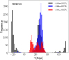 |
Fig. 1 Histograms show the distribution of the centroid time delay for Mrk1501 obtained with the FR/RSS method for thresholds 0.6 (black), 0.8 (blue), and 0.9 (red). |
2.3.3 Out-of-sample performance
One way to test how well a model generalises to future data is to evaluate its predictive performance on data that do not belong to training sample, such as test data. If the model predicts well based on out-of-sample data, this means that it has successfully captured certain aspects of the process underlying the observed data, that is, the model can generalise. The standard ICCF (as described in Sect. 2.2) does not provide predictions for out-of-sample data; such predictions would allow us to assess its generalisation performance and compare against alternative, competing models.
2.3.4 Absence of delay prior
The ICCF is often used together with the FR/RSS method to obtain a probability distribution for the delay. However, the FR/RSS method does not consider a prior distribution for the delay. The proposed GPCC considers a prior distribution for the delay. In particular, we give an example of a prior based on BLR photoionisation physics (see Sect. 2.5.2), which has the property of suppressing long delays that seem implausible. Previously, the alias mitigation technique was used to suppress long delays that occur due to a small number of overlapping points (e.g. Zajaček et al. 2021). However, alias mitigation suffers from the following issues: (a) it is not part of the respective probabilistic model formulations and yet it contributes to the calculation of the posterior, (b) it is not physically motivated, and (c) it cannot be interpreted as a prior because it depends on the data. Although our choice of prior may seem subjective, our method is not dependent on this particular choice and can indeed take alternative priors into consideration. However, discussing which physical prior is more appropriate is a more fruitful approach than devising weighting schemes based on heuristic motivation.
2.4 Assumptions of ICCF
In this section, we present the modelling assumptions underlying the ICCF method. The cross-correlation function between two time series y1(t) and y2(t) is a measure of their overlap and reads:
 (3)
(3)
where τ is denoted as the delay.
We consider two cases in which time series may be related. In the first case, we assume that the time series are related by y2(t - τ) = αy1(t) + b. That is, y2 is a scaled, offset, and delayed version of y1. If τ is unknown, we can estimate it as  . In this case, the maximum overlap between the two time series y1(t) and y2(t) at
  is an estimate of the lag that aligns the two time series.
In the second case, we consider a more general relation between two time series, y2 = 𝒯{y1}; for example, 𝒯 may stand for convolution with a function h such that  . In this case, y2(t) may have certain features (e.g. peaks or troughs) that also occur in y1(t) but at an earlier time. Therefore, y2(t) may look like a delayed version of y1(t) and we can use again arg maxτ(y1 ⋆ y2)(τ) to estimate this perceived lag between the respective features of the light curves. In this second case, we cannot find τ such that a delayed time series y2(t – τ) aligns with y1(t), because y2 is not simply a time-shifted version of y1 but a transformation of it described by 𝒯.
We argue that the ICCF relies on the assumption that the light curves are related by y2(t – τ) = αy1(t) + b, because this is the only case in which the maximum overlap coincides with an estimate of the delay between two time series. We also note that two time series related by y2(t – τ) = αy1(t) + b, with respect to a latent signal f (t) can be written as follows:
 (4)
(4)
where each time series yl(t) has its own scale al, offset bl, and delay tl.
Introducing a common latent signal ƒ(t), which is the unobserved driver of the observed time series, allows us to indirectly relate more than just two time series:
 (5)
(5)
These relations allow us to consider the joint estimation of multiple delays τ1,…, τL between L number of time series. Hence, when we use cross-correlation to reveal the delay between multiple light curves, we implicitly assume that they are related via a latent signal:
 (6)
(6)
2.5 Gaussian process cross-correlation
In this section, we propose to model ƒ (t) as a GP. This leads to a model that we refer to as Gaussian process cross-correlation (GPCC).
2.5.1 Model formulation
Based on Eq. (6), we assume that a common latent signal f(t) generates all observed light curves. Here we postulate that ƒ(t) ~ 𝒢Ƥ(0, kρ), meaning that ƒ (t) is drawn from a zero-mean GP with covariance function kρ(t, t′), where ρ is a scalar parameter. For two observed light curves, yi(t) and yj(t), we write:
 (7)
(7)
where ϵi,n is zero-mean Gaussian noise with standard deviation σi,n. We impose a Gaussian prior on the offset vector  . Given that ƒ(t) is drawn from a GP and that a GP is closed under affine transformations, the joint distribution of the observed light curves is also governed by a GP. To specify this GP, we need its mean and covariance function. Taking expectations over both priors 𝒢Ƥ(0, kρ) and p(b), we calculate the mean for the ith band:
![Mathematical equation: ${\mu _{{b_i}}} = {\rm{E}}\left[ {{y_i}\left( {{t_{i,n}}} \right)} \right].$](/articles/aa/full_html/2023/06/aa45932-23/aa45932-23-eq16.png) (8)
(8)
Taking again expectations over both priors, we calculate the covariance between the fluxes observed in the ith band and jth band2:
![Mathematical equation: $\matrix{ {c\left( {{t_{i,n}},{t_{j,m}}} \right) = {\rm{E}}\left[ {{y_i}\left( {{t_{i,n}}} \right) - {\mu _{{b_i}}}} \right]{\rm{E}}\left[ {{y_j}\left( {{t_{j,m}}} \right) - {\mu _{{b_j}}}} \right]} \hfill \cr {\quad \quad \quad \quad \, = {\alpha _i}{\alpha _j}{k_\rho }\left( {{t_{i,n}} - {\tau _i},{t_{j,m}} - {\tau _j}} \right)} \hfill \cr {\quad \quad \quad \quad \,\,\,\,\, + {\delta _{i,j}}\sigma _{{b_i}}^2 + {\delta _{i,j}}{\delta _{n,m}}\sigma _{i,n}^2.} \hfill \cr }$](/articles/aa/full_html/2023/06/aa45932-23/aa45932-23-eq17.png) (9)
(9)
Evaluating c(·, ·) at all the possible pairs that we can form by pairing the observations times ti,n in the ith band with tj,m in jth band results in a Ni × Nj covariance matrix C(ti, tj). We repeat this calculation for each of the (i, j) pairs of bands to obtain a number L2 of covariance matrices. We arrange these individual covariance matrices in a L × L block structure to form the N × N covariance matrix C(t, t) between all possible pairs of bands. For instance, for L = 2 bands, we would have:
 (10)
(10)
Hence, the (i, j)th block of C(t, t) has dimensions Ni × Nj and holds the covariances between the ith and jth light curves; the (n, m)th entry of the (i, j)th block is given by c(ti,n, tj,m).
Given the derived mean and covariance, the likelihood reads:
 (11)
(11)
Here, Q is an auxiliary N × L matrix with entries set to 0 or 1 (see Appendix A); it replicates the vector µb so that
![Mathematical equation: ${\bf{Q}}{{\bf{\mu }}_b} = \underbrace {\left[ {{\mu _{{b_1}}}, \ldots } \right.{\mu _{{b_1}}}}_{{N_1}}, \ldots ,\underbrace {\left. {{\mu _{{b_L}}}, \ldots ,{\mu _{{b_L}}}} \right].}_{{N_L}}$](/articles/aa/full_html/2023/06/aa45932-23/aa45932-23-eq20.png) (12)
(12)
Henceforth, we suppress in the notation the conditioning on t and σ and consider it implicit, that is, p(y|t, σ, τ, α,ρ) = p(y|τ, α,ρ). Finally, fitting the observed data involves maximising the likelihood p(y|τ, α, ρ) with respect to the free parameters α and ρ.
2.5.2 Prior on delay
The photoionisation physics define the ionisation parameter as
 (13)
(13)
where Q(H) is the number of photons per second emitted from the central source ionising the hydrogen cloud, r is the distance between the central source and the inner face of the cloud, and ηH is the total hydrogen density. Assuming that the BLRs for low luminosity Seyfert to high-luminosity quasars have the same ionisation parameter and BLR density, one can define an upper limit on the BLR size as a function of the AGN bolometric luminosity,
 (14)
(14)
As Lbol is in practice very difficult to measure, one can use bolometric corrections, for example, using the optical continuum luminosity measured at 5100 Å, LBol = 10λLλ(5100 Å) (McLure & Dunlop 2004). Bentz et al. (2013) provide a normalised expression for the Hβ BLR size for a given optical continuum luminosity:
![Mathematical equation: ${R_{{\rm{H}}\beta }}\left( {\lambda {L_\lambda }\left( {5100{\rm{{\AA}}}} \right)} \right) = {10^{1.559}}{\left[ {{{\lambda {L_\lambda }\left( {5100{\rm{{\AA}}}} \right)} \mathord{\left/ {\vphantom {{\lambda {L_\lambda }\left( {5100{\rm{{\AA}}}} \right)} {{{10}^{44}}}}} \right. \kern-\nulldelimiterspace} {{{10}^{44}}}}} \right]^{0.549}}\left[ {{\rm{light}} - {\rm{day}}} \right],$](/articles/aa/full_html/2023/06/aa45932-23/aa45932-23-eq23.png) (15)
(15)
where the slope value of 0.549 corresponds to the Clean2+ ExtCorr fit obtained from Bentz et al. (2013, their Table 14), which includes a special treatment of the sources and an additional extinction correction.
We define τmax(l, z) = RHβ(l)(1 + z)[light – day] as the upper limit on the delay measured in the observer frame, where we define l = 10λLλ(5100 Å) to simplify notation. As we have no further information, we assume the prior to be the uniform distribution:
 (16)
(16)
The uniform distribution is the maximum entropy probability distribution for a random variable about which the only known fact is its support.
2.5.3 Predictive likelihood for GPCC
We wish to compute the likelihood on new light curve data, that is, test data, as opposed to training data on which our model is already conditioned. Following the notation in Sect. 2.1, we denote test data with an asterisk such that ![Mathematical equation: ${{\bf{y}}^*} = \left[ {{\bf{y}}_1^*, \ldots ,{\bf{y}}_L^*} \right]$](/articles/aa/full_html/2023/06/aa45932-23/aa45932-23-eq25.png) , where each light curve
, where each light curve ![Mathematical equation: ${\bf{y}}_l^* = \left[ {{y^*}\left( {{t_{l,1}}} \right), \ldots ,{y^*}\left( {{t_{l,{N_l}}}} \right)} \right]\,\, \in \,\,{^{N_l^*}}$](/articles/aa/full_html/2023/06/aa45932-23/aa45932-23-eq26.png) is observed at times
is observed at times ![Mathematical equation: ${\bf{t}}_l^* = \left[ {t_{l,1}^*, \ldots ,t_{l,N_l^*}^*} \right]\,\, \in \,\,{^{N_l^*}}$](/articles/aa/full_html/2023/06/aa45932-23/aa45932-23-eq27.png) with measured errors
with measured errors ![Mathematical equation: ${\bf{\sigma }}_l^* = \left[ {\sigma _{l,1}^*, \ldots ,\sigma _{l,N_l^*}^*} \right]\,\, \in \,\,{^{N_l^*}}$](/articles/aa/full_html/2023/06/aa45932-23/aa45932-23-eq28.png) . Accordingly, we define
. Accordingly, we define  . We also define the cross-covariance function between training and test data
 (17)
(17)
which is identical to Eq. (9) after discarding its last term. Evaluating c* (·, ·) at all the possible pairs that we can form by pairing the observations times ti,n in the ¡th band with the test observation times  in jth band results in a
  covariance matrix
  . By repeating this for all (i, j) pairs of bands, we obtain L2 number of covariance matrices, which we arrange in a L × L block structure to form the N × N* covariance matrix C*(t, t*). For example, in the case of L = 2 bands we would have
 (18)
(18)
The predictive likelihood for the new data (test data) given the observed data (training data) is a Gaussian distribution3 (see Appendix B):
 (19)
(19)
where
 (20)
(20)
 (21)
(21)
The N* × L auxiliary matrix Q* replicates vector b so that:
![Mathematical equation: ${{\bf{Q}}^ * }{{\bf{\mu }}_b} = \underbrace {\left[ {{\mu _{{b_1}}}, \ldots ,} \right.{\mu _{{b_1}}}}_{N_1^ * }, \ldots ,\underbrace {\left. {{\mu _{{b_L}}}, \ldots ,{\mu _{{b_L}}}} \right].}_{N_L^ * }$](/articles/aa/full_html/2023/06/aa45932-23/aa45932-23-eq38.png) (22)
(22)
We construct the matrix Q* in the same way as the matrix Q, as shown in Appendix A. The N* × N* matrix C(t*, t*) is computed in the same way as the matrix C(t, t), that is, by evaluating c(·, ·) at all possible pairs  . For example, in the case of L = 2 bands we would have
 (23)
(23)
2.5.4 Posterior density for delays
Given a data set y t σ observed at L number of bands, we want to infer the posterior distribution for τ. We compute the non-normalised posterior of the delays over a finite regular grid of delay combinations, and then normalise these values into a multinomial distribution. We denote this grid and the multinomial posterior probabilities on the grid by

 (24)
(24)
with elements τi in the set {0, 1δτ, 2δτ,…, Tδτ}L. Here,  and
and  are the optimal parameters obtained when maximising the likelihood in Eq. (11) for each considered delay τi. As delays are relative to each other, for example delays τ1 = 0.3, τ2 = 1.3 are equivalent to τ1 = 0.0, τ2 = 1.0, without loss of generality, we fix the delay parameter of the first light curve to τ1 = 0.
3 Simulations
We present a simple numerical simulation with synthetic data that shows how the model behaves under perfect theoretical conditions; that is, when the data match our model assumptions.
We simulate data in two bands with a delay of τ = 2 days, where τ1 = 0, τ2 = 2. The remaining parameters are set as follows: α1 = 1, α2 = 1.5, b1 = 6, b2 = 15. We use the Ornstein-Uhlenbeck (OU) kernel  and set ρ = 3.5. For the first band, we sample 60 observation times from the uniform distribution 𝓊(0,20). For the second band, we sample 50 observation times from the two-component distribution 0.5𝓊(0,8) + 0.5𝓊(12,20), so that an observation gap is introduced between days 8 and 12. After sampling the observation times, we sample the latent signal f(t) ~ 𝒢Ƥ(0, kρ) and then the fluxes using Eq. (7). We perform four experiments in which we attempt to recover the delay under Gaussian noise using the respective standard deviations σ ∈ {0.l, 0.5, 1.0, 1.5}. As delays are relative to each other (e.g. delays τ1 = 0.3, τ2 = 1.3 are equivalent to τ1 = 0.0, τ2 = 1.0), we fix τ1 = 0.0 and seek only the second delay τ = τ2. We assume the prior p(τ) ∝ 1 and consider candidates τ in the grid {0,0.1,…, 30}, which has a step size of 0.1 days.
We show the results of the simulations in Fig. 2. The true peak at 2 days is identified in all experiments. For the values of σ = 1.0 and σ = 1.5, we see that alternative peaks arise as potential candidates. The reason these new peaks arise is that noise can suppress salient features, making light curves look more similar to each other. We note in particular that alternative peaks tend to arise at large delays, which we explain as follows. Small delays shift light curves only slightly so that they still overlap considerably after the shift (see left plot in Fig. C.2). For a small delay to be likely, the algorithm must match a number of features (i.e. peaks, troughs) appearing in one light curve to features appearing in the other. However, large delays shift light curves by so much that they overlap only slightly after the shift (see right plot in Fig. C.2). For a large delay to be likely, the algorithm must match fewer light-curve features than in the case of a small delay. Hence, it is “easier” for a large delay to arise as a candidate than it is for a small delay4.
We also observe that the posterior distribution becomes flat in the interval of [20,30] days. We reiterate that the simulated light curves span no longer than 20 days. A delay in [20,30] shifts the light curves so far apart that they no longer over-lap5 (see right plot in Fig. C.2). All large delays that lead to non-overlapping light curves yield the same covariance matrix (seeEq. 10),
 (25)
(25)
and therefore the same likelihood, which explains why the posterior distribution becomes flat after a certain delay and then remains so.
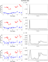 |
Fig. 2 Synthetic simulations with true delay at 2 days. The vertical axis is in arbitrary units of simulated flux. The left column shows the simulated light curves. The inferred posterior distribution of delay is shown in the right column. The noise σ increases from the top to the bottom row. |
4 Data applications
In this section, we apply our method to AGN data from RM campaigns for which time-delay measurements were made using the ICCF method. In particular, we focus on the sample of five AGN from Grier et al. (2012, hereafter G+2012) that provided high-sampling- rate light curves in the continuum (at 5100 Å) and in the Hβ emission line as part of a BLR RM campaign. For an application of the method to more than two light curves, we use the data obtained for MCG+08-11-011 as part of a RM monitoring of the AD by Fausnaugh et al. (2018).
In all applications, we employ the OU kernel  . Concerning the offset prior
  , we employ a prior centred on the sample means
  of the observed light curves, but with a highly inflated variance in order to render it only weakly informative, so that
  and
and  . Without loss of generality, we fix τ1 = 0.0 and seek only the second delay τ = τ2. In all applications, we consider candidate delays in the grid τ ∈ {0.0,0.2,…, 140}, which has a step size of 0.2 days.
Figure 3 shows the results for source 3C120. We present results for other sources in Appendix D. The posterior distribution of the delay obtained with the prior p(τ) ∝ 1 (middle panel, Fig. 3) broadly agrees with the ICCF (bottom panel, Fig. 3). Multiple peaks occur in the region between 10 and 40 days, which is consistent with the peak and centroid measured in the ICCF (values in bottom panel Fig. 3; see also Table 8 in G+2012). Higher probability peaks are observed at larger delays (>100 days), and may arise because of noise and the small number of overlapping points, as discussed in Sect. 3. A similar behaviour, which could be attributed to the same factors, is also observed in the ICCF for delays longer than ~80 days. We note that our range of the ICCF calculation is larger than that in G+2012 (their Fig. 4) and we consider delays closer to the length of the light curves. Based on the reported host-subtracted luminosity of 3C120, L5100å = (9.12 ± 1.15) × 1043 erg s−1 (see Table 9 in G+2012), we infer the posterior distribution of the delay using the prior p(τ) = 𝓊(0,τmax(l, Z)) as defined in Sect. 2.5.2 (top panel, Fig. 3). The introduction of the physically motivated prior (see Sect. 2.5.2) suppresses all peaks at larger delays and accentuates the peaks at lower delays. The peak of highest probability occurs at 27.6 days, which is close to the ICCF peak and centroid estimates.
Mass estimation for 3C120 and Mrk1501
The posterior distribution captures all possible solutions for the delay. This set of possible solutions can be incorporated into the calculation of other quantities. In the following, we use the recovered delay posterior (see top panel in Fig. 3) calculated with the prior presented in Sect. 2.5.2 to estimate the black-hole-mass distribution of 3C120 and Mrk1501. According to the virial theorem, the black hole mass MBH is given by
 (26)
(26)
where σV is the velocity dispersion of the emission lines, R = c • τ is the size of the BLR, and the factor ƒ depends on the geometry and kinematics of the BLR (Pozo Nuñez et al. 2014 and references therein). As in G+2012, we use the velocity dispersion given by the linewidth of the RMS residual spectrum, σV = 1514 ± 65 km s−1 (their table 9), and assume a scaling factor ƒ = 5. 5 (Onken et al. 2004). We show the resulting probability distribution for the black hole mass in Fig. 4. We emphasise that the distribution we calculate accounts for the uncertainty in the velocity dispersion σV. G+2012 reported an estimate of MBH = (6.7 ± 0.6) × 107 M⊙ obtained by error propagation of the delay and velocity dispersion in Eq. (26). As seen in Fig. 4, the two estimates agree closely. Nevertheless, we surmise that this close agreement seems to be due to the variance of the veSocity dispersion dominating the variance of the delay estimate. We provide further details in Appendix E.
Figure 5 shows the probability distribution for the black hole mass of Mrk1501. Again we use Eq. (26) to calculate the mass distribution, with values f = 5.5 and σV = 3321 ± 107 km s−1 and the corresponding delay posterior (seetop panel in Fig. D.1). The resulting distribution indicates that potential candidate values for the black hole mass concentrate around two distinct modes. G+2012 reported an estimate of MBH = (184 ± 27) × 106 M⊙, which is in good agreement with one of the modes of our estim ate.
As mentioned above, the variance in velocity dispemon dominates the variance in delay when calculating the distribution of MBH6. For example, for high-redshift quasrs, the uncertainty in the time delay increases considerably, which is mainly due to significant seasonal gaps and the decrease in the amplitude of the variability. This poses an additional challenge when using delay–luminosity scaling relations (e.g. based on the CIV line) to estimate black hole masses from a single-epoch spectrum (e.g. Kaspi et al. 2021; Grier et al. 2019). One could use very high-resolution spectroscopy (R ~ 20000) to improve the accuracy of the velocity dispersion to ~1% (e.g. Cazzoli et al. 2020). However, under such conditions, the uncertainty in the delay in Eq. (26) becomes relatively more influential and therefore an improved description of the delay posterior distribution would be important; this could be delivered by the GPCC.
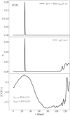 |
Fig. 3 GPCC application to 3C120. Top: posterior distribution of delay with prior p(τ) = 𝓊(0, τmax(l, Z)). The peak with the highest probability corresponds to a delay of 27.6 days. Middle: posterior distribution of delay with flat prior p(τ) ∝ 1. Bottom: ICCF calculated with a sampling of 1 day for linear interpolation of fluxes. The centroid is determined using the 80% rule. Our results for the ICCF peak and centroid are identical to those of G+2012, and we show the results of G+2012 including the uncertainty estimated with the FR/RSS method. All delays are indicated in the rest frame. |
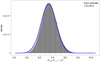 |
Fig. 4 Grey histogram is our probability distribution estimate for the black hole mass of 3C120. The blue line corresponds to the MBH = (6.7 ± 0.6) × 107 M⊙ estimate repшted in G+2012. |
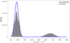 |
Fig. 5 Grey histogram is our probability distribution estimate for the black hole mass of Mrk1501. The blue line corresponds to the MBH = (184 ± 27) × 106 M⊙ estimate reported in G+2012. |
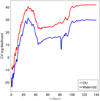 |
Fig. 6 Cross-validation results for 3C120: OU vs. Matern32. |
Model selection
The GPCC provides out-of-sample predictions (see Eq. (19)) and can therefore be subjected to model selection via cross validation. This allows us not only to compare GPCC to other models in terms of predictive performance, but also to validate certain choices when using GPCC, such as the kernel choice. We briefly demonstrate how cross validation allows us to decide which one of two candidate kernels7, OU or Matern32, provides a better fit for the datasets 3C120 and Mrk 6. We consider delays in {0.0,0.2,…, 140}. We perform 10-cross fold validation for each candidate delay. Figures 6 and 7 display the cross-validated log-likelihood for the two kernels. Evidently, the kernels perform similarly, but the OU kernel shows consistently better performance and is therefore the better choice of the two. We note that this kind of model selection is not possible in the case of the ICCF – for instance, we may want to choose between two ways of interpolating the observed fluxes – as it does not provide out-of-sample predictions.
Three light curves, MGC+08-11-011
As an example of the analysis of more than two light curves, we use the data published in Fausnaugh et al. (2018) for the source MCG+08-11-011 as part of a RM campaign of the AD. We use the light curves at bands 5100 Å, and the Sloan i and z with central wavelengths at 7700 Å, and 9100 Å, respectively. We consider delays in {0,0.1,…, 10}. Here, the maximum delay of 10 days is well above the delay predicted by standard AD theory (e.g. Pozo Nuñez et al. 2019, Pozo Nuñez et al. 2023). The joint posterior is shown in Fig. 8. The orientation of the joint posterior distribution reveals a positive correlation between the delays.
As pointed out in Sect. 2.3.1, this is a case where GPCC has an advantage over ICCF as the latter cannot produce a joint estimate of the two sought delays, but must instead consider pairs of light curves at a time. Moreover, this pairwise estimation may lead to an inconsistency. To demonstrate this inconsistency, we use the GPCC to estimate the delays between the three pairs of light curves 5100 Å and 7700 Å, 5100 Å and 9100 Å, and 7700 Å and 9100 Å, as opposed to the joint estimation that we show above. We display the results of this pairwise estimation in Fig. 9 (top). The results tell us that the mean delay between 5100 Å and 7700 Å is 1.29 days (red), and that the mean delay between 5100 Å and 9100 Å is 1.23 days (blue). Given these two pieces of information, we would expect the mean delay between 7700 Å and 9100 Å to be approximately8 1.23−1.29 = −0.06 days, but the pairwise comparison yields a mean of 0.71 days (black). Hence, the pairwise estimation leads to an inconsistency as the distribution of the pairwise delays suggests that the mean delay for 7700 Å and 9100 Å should be closer to 0.06 days rather than the independently estimated 0.71 days. For comparison, we display in Fig. 9 (bottom) the marginals of the delay distribution calculated from the joint posterior in Fig. 8. The figure shows that the mean delay between 5100 Å and 7700 Å is 1.31 days (red), and that the mean delay between 5100 Å and 9100 Å is 1.61 days (blue), which is consistent with the mean delay of 0.33 (black) between 7700 Å and 9100 Å.
5 Summary and conclusions
We present a probabilistic reformulation of the ICCF method to estimate time delays in RM of AGN. The main features and advantages of our method can be summarised as follows:
- –
It accounts for observational noise and provides a posterior probability density of the delay. The ICCF provides only a point estimate for the delay. A distribution for the delay can be obtained using the bootstrapping method as implemented in FR/RSS, but it has the disadvantage of being susceptible to the removal of individual data points. The posterior distribution obtained in the Bayesian framework is a powerful alternative to bootstrapping;
- –
When using the ICCF, one has to manually choose an object-dependent threshold to determine the peak and centroid of the cross-correlation curve. The proposed model avoids such manual choices by relying on a probabilistic formulation that defines a cost function, the marginal log-likelihood. This guides the optimisation of the parameters and is used in the derivation of the posterior density for the delay;
- –
The proposed model can jointly estimate the delay between more than two light curves, a task that cannot be accomplished with the ICCF. The ICCF follows a pairwise estimation approach that can lead to delays that are inconsistent with each other;
- –
Finally, we demonstrate that the capability of the proposed model for out-of-sample predictions allows us to use cross validation to choose the kernel. Similarly, we could have used cross-validation to call into question other design choices of the model such as the noise model. The same capability would also allow us to pit our proposed model against other competing models in a cross-validation framework in order to decide which one best fits the observed data at hand. The ICCF does not possess this capability.
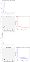 |
Fig. 8 Joint delay posteriors for MGC+08-11-011. |
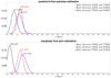 |
Fig. 9 Pairwise (top) and joint (bottom) estimation of delays. Each density is given its mean and standard deviation. We note that the two estimation methods give different results when the delays are estimated for three light curves in MGC +08-11-011. |
Acknowledgements
The authors gratefully acknowledge the generous and invaluable support of the Klaus Tschira Foundation. F.P.N. warmly thanks Bozena Czerny for discussions. This project has received funding from the European Research Council (ERC) under the European Union’s Horizon 2020 research and innovation programme (grant agreement no. 951549). This research has made use of the NASA/IPAC Extragalactic Database (NED) which is operated by the Jet Propulsion Laboratory, California Institute of Technology, under contract with the National Aeronautics and Space Administration. This research has made use of the SIMBAD database, operated at CDS, Strasbourg, France. We thank the anonymous referee for constructive comments and careful review of the manuscript.
Appendix A Matrix Q
Matrix Q has dimensions N × L. Its lth column reads:

We construct the columns of the N* × L matrix Q*, used when calculating the predictive likelihood in Equation (19), in the exact same fashion.
Appendix B Predictive likelihood
The joint distribution of observed fluxes and new fluxes reads:
 (B.1)
(B.1)
By conditioning on y, we obtain Equation (19) from Equation (B.1).
Appendix C Simulations
Figure C.1 shows an example of the ICCF application to simulated data. Figure C.2 shows how the synthetic curves, considered in Section 3, align for candidate posterior delays for the case of σ = 1.5.
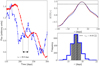 |
Fig. C.1 ICCF application to simulated data. Left panel: AD continuum light curve (blue) modelled as a random walk process with a power spectral density P(ν) ∝ ν−2 (Kelly et al. 2009; Caplar et al. 2017). The delayed BLR emission line light curve (red) is obtained by convolving the AD light curve with a rectangular transfer function over the time domain, t ∈[τ0 − ∆τ/2, τ0 + ∆τ/2] where ∆τ/τ0 ≤ 2 (Pozo Nuñez et al. 2013). For this particular example, a centroid τ0 = 20 days is assumed. Both light curves were randomly sampled, with an average sampling of 1 day and noise level of 1% (S/N = 100). Right Upper Panel: ICCF results when the line is interpolated and the continuum is shifted (blue) and when the continuum is interpolated and the line is shifted (red). The average ICCF is shown in black. The dotted black line marks the threshold of 0.8max(ICCF) used to calculate the centroid. Right bottom panel: The histogram shows the distribution of the centroid delay obtained by the FR/RSS method (see text). The black area marks the 68% confidence range used to calculate the errors of the centroid. |
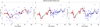 |
Fig. C.2 Synthetic light curves for σ = 1.5 aligned with delays 2 (left), 16.8 (middle), and 20 (right). Vertical axis is in arbitrary units of simulated flux. The black line is the recovered latent signal f(t) that underlies all observations (see 2.5.1). All three delays lead to plausible alignments. |
Appendix D Individual sources
Appendix E Mass distribution of 3C120 for fixed delay
We display an additional figure that shows the mass distribution of 3C120 calculated using Equation (26) but with the delay τ fixed to its mean posterior value of 27.4 and allowing only the velocity dispersion to vary according its Gaussian distribution implied by σV = 1514 ± 65 km/s. We note that Figure E.1 is almost identical to Figure 4. The standard deviation of our distribution (grey histogram) for fixed delay in Figure E.1 is 0.580 × 10⁷, while the standard deviation of our distribution in Figure 4 (again grey histogram) has an only slightly larger value of 0.596 × 10⁷. This suggests that the variance of the velocity dispersion dominates the variance of the delay. We surmise that this is the reason that our estimate and the G+2012 estimate appear to be in close agreement even though the corresponding black-hole-mass estimates might agree to a lesser extent.
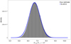 |
Fig. E.1 Probability density estimate for the black hole mass of 3C120 when fixing the delay τ to its posterior mean value of 27.4 days (grey histogram). The observed variance of the grey histogram is entirely due to the variance of the velocity dispersion as delay τ is fixed to its mean posterior value. The blue line corresponds to the Gaussian probability density Mbh = (6.7 ± 0.6) × 107 M⊙ reported in G+2012. |
References
- Alexander, T. 1997, Astron. Time Ser., 218, 163 [CrossRef] [Google Scholar]
- Almeyda, T., Robinson, A., Richmond, M., et al. 2020, ApJ, 891, 26 [CrossRef] [Google Scholar]
- Bentz, M. C., Denney, K. D., Grier, C. J., et al. 2013, ApJ, 767, 149 [Google Scholar]
- Blandford, R. D. & McKee, C. F. 1982, ApJ, 255, 419 [CrossRef] [Google Scholar]
- Cackett, E. M., Gelbord, J., Li, Y.-R., et al. 2020, ApJ, 896, 1 [NASA ADS] [CrossRef] [Google Scholar]
- Cackett, E. M., Bentz, M. C., & Kara, E. 2021, iScience, 24, 102557 [NASA ADS] [CrossRef] [Google Scholar]
- Caplar, N., Lilly, S. J., & Trakhtenbrot, B. 2017, ApJ, 834, 111 [NASA ADS] [CrossRef] [Google Scholar]
- Cazzoli, S., Gil de Paz, A., Márquez, I., et al. 2020, MNRAS, 493, 3656 [NASA ADS] [CrossRef] [Google Scholar]
- Chelouche, D., Pozo-Nuñez, F., & Zucker, S. 2017, ApJ, 844, 146 [CrossRef] [Google Scholar]
- Cherepashchuk, A. M., & Lyutyi, V. M. 1973, Astrophys. Lett., 13, 165 [NASA ADS] [Google Scholar]
- Edelson, R. A., & Krolik, J. H. 1988, ApJ, 333, 646 [Google Scholar]
- Fausnaugh, M. M., Starkey, D. A., Horne, K., et al. 2018, ApJ, 854, 107 [NASA ADS] [CrossRef] [Google Scholar]
- Gaskell, C. M., & Peterson, B. M. 1987, ApJS, 65, 1 [NASA ADS] [CrossRef] [Google Scholar]
- Gaskell, C. M., & Sparke, L. S. 1986, ApJ, 305, 175 [NASA ADS] [CrossRef] [Google Scholar]
- Grier, C. J., Peterson, B. M., Pogge, R. W., et al. 2012, ApJ, 755, 60 [NASA ADS] [CrossRef] [Google Scholar]
- Grier, C. J., Peterson, B. M., Horne, K., et al. 2013, ApJ, 764, 47 [NASA ADS] [CrossRef] [Google Scholar]
- Grier, C. J., Trump, J. R., Shen, Y., et al. 2017, ApJ, 851, 21 [NASA ADS] [CrossRef] [Google Scholar]
- Grier, C. J., Shen, Y., Horne, K., et al. 2019, ApJ, 887, 38 [NASA ADS] [CrossRef] [Google Scholar]
- Kaspi, S., Brandt, W. N., Maoz, D., et al. 2021, ApJ, 915, 129 [NASA ADS] [CrossRef] [Google Scholar]
- Kelly, B. C., Bechtold, J., & Siemiginowska, A. 2009, ApJ, 698, 895 [Google Scholar]
- Koratkar, A. P., & Gaskell, C. M. 1991, ApJS, 75, 719 [NASA ADS] [CrossRef] [Google Scholar]
- Kozłowski, S., Kochanek, C. S., Udalski, A., et al. 2010, ApJ, 708, 927 [CrossRef] [Google Scholar]
- Landt, H., Ward, M. J., Kynoch, D., et al. 2019, MNRAS, 489, 1572 [NASA ADS] [CrossRef] [Google Scholar]
- McLure, R. J., & Dunlop, J. S. 2004, MNRAS, 352, 1390 [NASA ADS] [CrossRef] [Google Scholar]
- Onken, C. A., Ferrarese, L., Merritt, D., et al. 2004, ApJ, 615, 645 [Google Scholar]
- Pancoast, A., Brewer, B. J., Treu, T., et al. 2012, ApJ, 754, 49 [NASA ADS] [CrossRef] [Google Scholar]
- Peterson, B. M., Wanders, I., Horne, K., et al. 1998, PASP, 110, 660 [Google Scholar]
- Peterson, B. M., Ferrarese, L., Gilbert, K. M., et al. 2004, ApJ, 613, 682 [Google Scholar]
- Pozo Nuñez, F., Ramolla, M., Westhues, C., et al. 2012, A&A, 545, A84 [NASA ADS] [CrossRef] [EDP Sciences] [Google Scholar]
- Pozo Nuñez, F., Westhues, C., Ramolla, M., et al. 2013, A&A, 552, A1 [NASA ADS] [CrossRef] [EDP Sciences] [Google Scholar]
- Pozo Nuñez, F., Haas, M., Ramolla, M., et al. 2014, A&A, 568, A36 [NASA ADS] [CrossRef] [EDP Sciences] [Google Scholar]
- Pozo Nuñez, F., Ramolla, M., Westhues, C., et al. 2015, A&A, 576, A73 [NASA ADS] [CrossRef] [EDP Sciences] [Google Scholar]
- Pozo Nuñez, F., Gianniotis, N., Blex, J., et al. 2019, MNRAS, 490, 3936 [Google Scholar]
- Pozo Nuñez, F., Bruckmann, C., Desamutara, S., et al. 2023, MNRAS, 522, 2002 [CrossRef] [Google Scholar]
- Rybicki, G. B., & Press, W. H. 1992, ApJ, 398, 169 [CrossRef] [Google Scholar]
- Welsh, W. F. 1999, PASP, 111, 1347 [Google Scholar]
- Zajaček, M., Czerny, B., Martinez-Aldama, M. L., et al. 2021, ApJ, 912, 10 [CrossRef] [Google Scholar]
- Zu, Y., Kochanek, C. S., & Peterson, B. M. 2011, ApJ, 735, 80 [NASA ADS] [CrossRef] [Google Scholar]
- Zu, Y., Kochanek, C. S., Kozłowski, S., et al. 2016, ApJ, 819, 122 [NASA ADS] [CrossRef] [Google Scholar]
Considering the Poisson probability that no particular point is selected, the size of the selected sample is reduced by a factor of about 1/e, resulting in 63% of the original data (see Peterson et al. 2004).
The Kronecker delta δij equals 1 when i = j, otherwise 0.
We suppress in the notation the conditioning on t, σ, t*, σ*.
Alias mitigation (e.g. Grier et al. 2017; Zajaček et al. 2021) has been used previously to address the situation where a small number of overlapping points leads to peaks in the distribution of delays.
Unlike the ICCF, such a delay is allowed in our formulation and the model assigns a probability to it.
We note that the geometry effects contained in the scaling factor f are the main source of uncertaibty in the estimates of the black hole mass from RM.
Alternative sets of kernels can be included in the model selection.
We note that comparing the means of the distributions of delays is only an approximate way of checking whether the estimated delays are consistent with one another.
All Figures
|
Fig. 1 Histograms show the distribution of the centroid time delay for Mrk1501 obtained with the FR/RSS method for thresholds 0.6 (black), 0.8 (blue), and 0.9 (red). |
| In the text | |
|
Fig. 2 Synthetic simulations with true delay at 2 days. The vertical axis is in arbitrary units of simulated flux. The left column shows the simulated light curves. The inferred posterior distribution of delay is shown in the right column. The noise σ increases from the top to the bottom row. |
| In the text | |
|
Fig. 3 GPCC application to 3C120. Top: posterior distribution of delay with prior p(τ) = 𝓊(0, τmax(l, Z)). The peak with the highest probability corresponds to a delay of 27.6 days. Middle: posterior distribution of delay with flat prior p(τ) ∝ 1. Bottom: ICCF calculated with a sampling of 1 day for linear interpolation of fluxes. The centroid is determined using the 80% rule. Our results for the ICCF peak and centroid are identical to those of G+2012, and we show the results of G+2012 including the uncertainty estimated with the FR/RSS method. All delays are indicated in the rest frame. |
| In the text | |
|
Fig. 4 Grey histogram is our probability distribution estimate for the black hole mass of 3C120. The blue line corresponds to the MBH = (6.7 ± 0.6) × 107 M⊙ estimate repшted in G+2012. |
| In the text | |
|
Fig. 5 Grey histogram is our probability distribution estimate for the black hole mass of Mrk1501. The blue line corresponds to the MBH = (184 ± 27) × 106 M⊙ estimate reported in G+2012. |
| In the text | |
|
Fig. 6 Cross-validation results for 3C120: OU vs. Matern32. |
| In the text | |
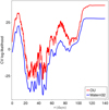 |
Fig. 7 Same as Fig. 6 but for Mrk6. |
| In the text | |
|
Fig. 8 Joint delay posteriors for MGC+08-11-011. |
| In the text | |
|
Fig. 9 Pairwise (top) and joint (bottom) estimation of delays. Each density is given its mean and standard deviation. We note that the two estimation methods give different results when the delays are estimated for three light curves in MGC +08-11-011. |
| In the text | |
|
Fig. C.1 ICCF application to simulated data. Left panel: AD continuum light curve (blue) modelled as a random walk process with a power spectral density P(ν) ∝ ν−2 (Kelly et al. 2009; Caplar et al. 2017). The delayed BLR emission line light curve (red) is obtained by convolving the AD light curve with a rectangular transfer function over the time domain, t ∈[τ0 − ∆τ/2, τ0 + ∆τ/2] where ∆τ/τ0 ≤ 2 (Pozo Nuñez et al. 2013). For this particular example, a centroid τ0 = 20 days is assumed. Both light curves were randomly sampled, with an average sampling of 1 day and noise level of 1% (S/N = 100). Right Upper Panel: ICCF results when the line is interpolated and the continuum is shifted (blue) and when the continuum is interpolated and the line is shifted (red). The average ICCF is shown in black. The dotted black line marks the threshold of 0.8max(ICCF) used to calculate the centroid. Right bottom panel: The histogram shows the distribution of the centroid delay obtained by the FR/RSS method (see text). The black area marks the 68% confidence range used to calculate the errors of the centroid. |
| In the text | |
|
Fig. C.2 Synthetic light curves for σ = 1.5 aligned with delays 2 (left), 16.8 (middle), and 20 (right). Vertical axis is in arbitrary units of simulated flux. The black line is the recovered latent signal f(t) that underlies all observations (see 2.5.1). All three delays lead to plausible alignments. |
| In the text | |
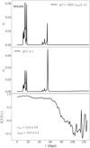 |
Fig. D.1 Same as Figure 3 but for Mrk1501. |
| In the text | |
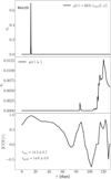 |
Fig. D.2 Same as Figure 3 but for Mrk335. |
| In the text | |
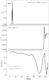 |
Fig. D.3 Same as Figure 3 but for Mrk6. |
| In the text | |
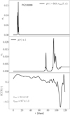 |
Fig. D.4 Same as Figure 3 but for PG2130+099. |
| In the text | |
|
Fig. E.1 Probability density estimate for the black hole mass of 3C120 when fixing the delay τ to its posterior mean value of 27.4 days (grey histogram). The observed variance of the grey histogram is entirely due to the variance of the velocity dispersion as delay τ is fixed to its mean posterior value. The blue line corresponds to the Gaussian probability density Mbh = (6.7 ± 0.6) × 107 M⊙ reported in G+2012. |
| In the text | |
Current usage metrics show cumulative count of Article Views (full-text article views including HTML views, PDF and ePub downloads, according to the available data) and Abstracts Views on Vision4Press platform.
Data correspond to usage on the plateform after 2015. The current usage metrics is available 48-96 hours after online publication and is updated daily on week days.
Initial download of the metrics may take a while.