| Issue |
A&A
Volume 674, June 2023
|
|
|---|---|---|
| Article Number | A87 | |
| Number of page(s) | 7 | |
| Section | Cosmology (including clusters of galaxies) | |
| DOI | https://doi.org/10.1051/0004-6361/202345886 | |
| Published online | 06 June 2023 | |
Turnaround density evolution encodes cosmology in simulations
1
Department of Physics and Institute for Theoretical and Computational Physics, University of Crete, 70013 Heraklio, Greece
e-mail: This email address is being protected from spambots. You need JavaScript enabled to view it.
2
Institute of Astrophysics, Foundation for Research and Technology – Hellas, Vassilika Vouton, 70013 Heraklio, Greece
Received:
11
January
2023
Accepted:
6
April
2023
Abstract
Context. The mean matter density within the turnaround radius, which is the boundary that separates a nonexpanding structure from the Hubble flow, was recently proposed as a novel cosmological probe. According to the spherical collapse model, the evolution with cosmic time of this turnaround density, ρta(z), can be used to determine both Ωm and ΩΛ, independently of any other currently used probe. The properties of ρta predicted by the spherical collapse model (universality for clusters of any mass, value) were also shown to persist in the presence of full three-dimensional effects in ΛCDM N-body cosmological simulations when considering galaxy clusters at the present time, z = 0. However, a small offset was discovered between the spherical-collapse prediction of the value of ρta at z = 0 and its value measured in simulations.
Aims. In this letter, we explore whether this offset evolves with cosmic time; whether it differs in different cosmologies; whether its origin can be confidently identified; and whether it can be corrected. Specifically, we aim to examine whether the evolution of ρta can be used to distinguish between simulated universes with and without a cosmological constant.
Methods. We used N-body simulations with different cosmological parameters to trace the evolution of the turnaround density ρta with cosmic time for the largest dark matter halos in the simulated boxes. To this end, we analyzed snapshots of these simulations at various redshifts, and we used radial velocity profiles to identify the turnaround radius within which we measured ρta.
Results. We found an offset between the prediction of the spherical collapse model for ρta and its measured value from simulations. The offset evolves slightly with redshift. This offset correlates strongly with the deviation from spherical symmetry of the dark matter halo distribution inside and outside of the turnaround radius. We used an appropriate metric to quantify deviations in the environment of a structure from spherical symmetry. We found that using this metric, we can construct a sphericity-selected sample of halos for which the offset of ρta from the spherical collapse prediction is zero, independently of redshift and cosmology.
Conclusions. We found that a sphericity-selected halo sample allows us to recover the simulated cosmology, and we conclude that the turnaround density evolution indeed encodes the cosmology in N-body simulations.
Key words: galaxies: clusters: general / cosmological parameters / large-scale structure of Universe / galaxies: halos / methods: numerical
© The Authors 2023
 Open Access article, published by EDP Sciences, under the terms of the Creative Commons Attribution License (https://creativecommons.org/licenses/by/4.0), which permits unrestricted use, distribution, and reproduction in any medium, provided the original work is properly cited.
This article is published in open access under the Subscribe to Open model. This email address is being protected from spambots. You need JavaScript enabled to view it. to support open access publication.
1. Introduction
The question of assigning meaningful boundaries to large-scale structures has traditionally been addressed via two distinct paths. The first path involves overdensity criteria: The boundary of the structure is defined as the scale at which the average matter density becomes some given multiple of the mean matter density, or of the critical density, of the Universe at the time of observation. Overdensity boundaries are motivated by the spherical collapse model (e.g., Gunn et al. 1972; Gunn 1977; Lahav et al. 1991). The second path involves kinematic or dynamic criteria, motivated by the study of infall onto existing collapsed structures (e.g., Fillmore & Goldreich 1984; Bertschinger 1985). Most recently, this approach motivated the introduction of the splashback radius (Diemer & Kravtsov 2014; Adhikari et al. 2014; More et al. 2015) as a boundary for structures that are still accreting matter from their environment.
A hybrid of the two types of boundaries is the turnaround radius, which is a kinematically motivated boundary (the scale that separates a nonexpanding structure from the Hubble flow) that according to spherical collapse, also constitutes a scale of constant overdensity for collapsed structures of all masses at a given redshift. In recent years, the turnaround radius has gained considerable attention as a scale on which cosmological models can be tested (e.g., Pavlidou & Tomaras 2014; Tanoglidis et al. 2015, 2016; Nojiri et al. 2018; Capozziello et al. 2019; Lopes et al. 2019; Wong 2019; Pavlidou et al. 2020; Santa Vélez & Enea Romano 2020; Del Popolo 2020; Faraoni et al. 2020; Korkidis et al. 2020; Lee & Baldi 2022).
Pavlidou et al. (2020) showed by employing the spherical-collapse model that the matter density within the turnaround scale (the turnaround density, ρta) could be used as a cosmology-probing observable, with a number of attractive properties: For a given redshift, the turnaround density is universal and thus insensitive to halo size, selection biases, and sample completeness issues; its present-day value almost exclusively probes the matter density; and its evolution with redshift is sensitive to the dark energy content of the Universe.
At the same time, the assumption of spherical symmetry implicitly used in Pavlidou et al. (2020) contradicts the highly nonspherical nature of realistic cosmological structures, raising serious concerns about the practical utility of ρta as a quantitative cosmological probe. However, Korkidis et al. (2020) showed with the aid of ΛSCDM cosmological N-body simulations that at the present time (z = 0), a dynamically meaningful turnaround radius can be measured kinematically from radially averaged velocity profiles for realistic cosmological structures. The average matter density within that scale was also shown to have a value that is very close to the value predicted by the spherical-collapse model. These results were consistent with earlier studies of simulated structures on similar scales (e.g., Busha et al. 2005; Cupani et al. 2008).
In this paper, extending the work of Korkidis et al. (2020), we aim to show that this agreement between the turnaround dynamics in realistic 3D structures and the spherical-collapse model persists for higher redshifts and for cosmological simulations with underlying cosmologies different from the concordance ΛSCDM. In Korkidis et al. (2020), the kinematically measured ρta had a systematic offset with respect to the prediction of the spherical collapse model. This offset would make the turnaround density problematic as a cosmological observable. In principle, this offset might be calibrated away using simulations before comparing with observations of clusters. However, this would be increasingly complicated if the offset depended on redshift and/or cosmology, and it would be impractical if these dependences were such that they would cause ρta(z) curves of different cosmologies to appear similar. The ideal situation would be to identify the origin of the offset and, if possible, eliminate it by applying appropriate quality cuts to the cluster sample used to constrain the cosmological parameters. Exploring these possibilities is a second objective of this work.
This paper is organized as follows: In Sect. 2 we describe the cosmological N-body simulations that we employed, the halo sample we used, and the method for calculating the turnaround density. In Sect. 3 we present our results. Specifically we show how ρta evolves with cosmic time for different cosmologies; how the offset of ρta(z) from spherical-collapse predictions changes with redshift and cosmology; that the offset, as would intuitively be expected, is dependent on the distribution of neighboring halos in the vicinity of the turnaround radius of a structure, and that we can use this fact to design appropriate cluster selection criteria for the elimination of the offset. We summarize and discuss our findings in Sect. 4.
2. Simulated data and methods
2.1. Cosmological N-body simulations
In this section, we describe the cosmological simulations that we used in our analysis along with the methods that we employed in order to measure the matter density at turnaround ρta. One of the main characteristics of the turnaround density in the spherical collapse model is that its evolution with cosmic time is sensitive to the presence of a cosmological constant. Thus, one of our objectives is to show that in N-body cosmological simulations, the kinematically measured ρta is also sensitive to the input cosmological parameters. To this effect, we analyze simulated halos from simulations assuming three different cosmologies: two flat models with Ωm ∼ 0.3 and ΩΛ ∼ 0.7 (referred to as ΛSCDM), an open-matter-only model with Ωm ∼ 0.3 and no cosmological constant (OCDM), and a flat-matter-only model, with Ωm = 1 and no cosmological constant (SCDM).
One of our ΛSCDM dark-matter-only boxes was taken from the MupltiDark Planck simulations (MDPL; Klypin et al. 2016), and it spans L = 1000 h−1 Mpc on a side. This particular run followed the evolution of 38403 particles with individual masses of Mp = 1.51 × 10⁹ h−1 M⊙ (MDPL2) and a cosmology consistent with Plank measurements (Planck Collaboration XIII 2016; see Table 1).
Cosmological parameters used in each simulation.
The second ΛSCDM box as well as the OCDM and SCDM simulations we analyzed were taken from the Virgo consortium1 suit of cosmological simulations. In particular, we analyzed their intermediate-sized N-body runs, which follow the evolution of 2563 particles with mass Mp = 6.86/22.7 × 1010 h−1 M⊙ (ΛCDM, OCDM/SCDM) in a box of L = 239.5 h−1 Mpc on a side.
Our choice to analyze older cosmological runs was driven by efficiency considerations (using available data rather than unnecessarily performing N-body runs from scratch) in combination with the fact that as recent cosmological data disfavor cosmologies other than ΛSCDM, virtually all currently produced publicly available datasets are small variations of ΛCDM, as effort has shifted toward running cosmological boxes with increasingly complex baryonic physics, or nonstandard dark matter models.
While no longer meeting the needs of most current cosmology projects in terms of their box size and resolution, the Virgo simulations were at the frontier of cosmological research at the time they were made publicly available, and they have been widely used and tested. We therefore chose to work with this very thoroughly explored set of cosmological runs because they are already publicly available and include models that are sufficiently different from the currently preferred concordance flat ΛSCDM so that the sensitivity of ρta(z) to cosmological parameters can be tested effectively. We additionally emphasize that the implementation of gravity in cosmological simulations has not changed since the Virgo runs, so given that our box size and resolution requirements are satisfied, the Virgo runs are adequate for our purposes.
Regarding halo identification, in the case of the MDPL2 box, the halo catalog was produced using the Rockstar algorithm (Behroozi et al. 2013). For the Virgo simulations, we used the friends-of-friends algorithm (FoF; Davis et al. 1985) using nbodykit2, and then we implemented a spherical overdensity (SO) criterion to calculate M200 masses for the identified halos. The snapshots that we used from both suits of simulations were in the range 0 ≤ z ≤ 13.
2.2. Turnaround density calculation, halo sampling, and substructure elimination
To calculate the turnaround density in simulations, the turnaround radius (the cluster-centric distance at which dark matter particles (on average) join the Hubble flow) and the turnaround mass (the total mass enclosed by the turnaround radius) have to be measured. In Korkidis et al. (2020) we showed that the turnaround radius for group- and cluster-sized halos is well defined as the radial shell for which the average radial velocity of dark matter particles, ⟨Vr⟩, crosses zero for the first time as the distance from the center of the cluster decreases. This shell also lies in a region in which the velocity dispersion  is minimum. This feature can also be identified in particle phase-space diagrams of cluster-sized halos (e.g., Cuesta et al. 2008; Vogelsberger & White 2011).
At each redshift snapshot of the Virgo simulations, we analyzed the 1000 most massive halos. At z = 0, this corresponded to halos with masses in the interval 1014 M⊙ ≤ M200 ≤ 1015 M⊙. Most of them lie at the lower limit. For each of these halos, we calculated the turnaround radius, Rta, and then proceeded to identify substructures within this scale.
For this task, we followed the analysis of Korkidis et al. (2020), where for each of our halos, we identified all neighboring halos within its Rta and labeled as “structures” hose with the largest M200, discarding the remaining “substructure” halos from further analysis. Through this cleaning procedure, 3 − 7% of the structures at each redshift were discarded as substructures for all of our simulated boxes.
A similar strategy was also followed for the MDPL2 simulation, but because in this case the simulated box was considerably larger, we followed a different approach to select the halo sample. In particular, we considered two samples: one sample with the 3000 most massive halos of the box (1014 M⊙ ≤ M200 ≤ 6 × 10¹⁵ M⊙), and a second sample for which we randomly selected 780 halos from logarithmically spaced mass bins, with M200 ≥ Mmin. The value for Mmin at each redshift snapshot scaled proportionately to the mass of the largest halo at that time, and was equal to 6 × 10¹³ M⊙ for z = 0.
The reasoning for choosing a random sample extending to low masses was twofold. On the one hand, we wished to examine a large enough dynamical range in mass (at least two orders of magnitude) so as to be able to identify any mass-driven effects or correlations. On the other hand, because of the enormous size of the halo catalog, we had to use some trimming-down algorithm for the halo catalogue to keep our analysis computationally tractable.
3. Results
3.1. Offset of the turnaround density in simulations from the spherical collapse prediction evolves with cosmic time
In Korkidis et al. (2020), we showed that the turnaround radius Rta is well correlated with the turnaround mass Mta, with a scaling very close to  , so that a meaningful characteristic turnaround density exists for z = 0 in a ΛCDM cosmology. We have confirmed that this remains true across redshifts and cosmologies (see Appendix A). In this section, we compare the value of this characteristic (average) turnaround density with spherical-collapse predictions.
The data points in the upper panel of Fig. 1 depict the evolution of the turnaround density with redshift for the three Virgo cosmologies and for MDPL2. The density was normalized with respect to the present-day value of the critical density ρcrit, 0 in each cosmology. The solid lines represent the evolution of Ωta, with z predicted from the spherical-collapse model (Pavlidou et al. 2020) in each cosmology.
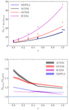 |
Fig. 1. Evolution of the turnaround density with redshift. Upper panel: data points: Ωta vs. redshift for the three Virgo cosmologies [ΛSCDM (black points), OCDM (red points), and SCDM (magenta points)] and for the MDPL2 ΛSCDM run. Each point corresponds to the mean value of Ωta in the halo sample at that z, and the error bars (in most cases smaller than the symbol size) correspond to the standard error on the mean. Solid lines: spherical-collapse prediction for Ωta vs. z for the corresponding cosmology. Lower panel: ratio of Ωta in simulations over the spherical-collapse prediction as a function of z for the Virgo and MDPL2 simulations. There is a small, evolving offset between the kinematically measured turnaround density in simulated halos and the spherical-collapse prediction. |
From the figure, two things are apparent for all three cosmologies: (a) As early as z = 0.3 − 0.5, the Ωta values of different cosmologies start to diverge. (b) There is a systematic offset between the simulation points and the spherical-collapse lines that evolves (decreases) weakly with cosmic time.
The second point is made more clear in the lower panel of Fig. 1, where we plot the ratio of Ωta from simulations and its predicted value from the spherical collapse model. Black, red, and magenta shaded regions represent the mean values of the simulations plus or minus one standard error for the three Virgo runs, while blue corresponds to the results from the MDPL2 simulation. Even accounting for halo-to-halo spread, it is clear that for all simulation suits, the offset decreases with increasing redshift. For the Virgo simulations, the offsets for ΛSCDM and OCDM are very similar up to z = 0.3, while the SCDM offset is much lower at all redshifts and even becomes negligible for high z. The MDPL2 simulation appears to have a much smaller offset than its Virgo ΛSCDM counterpart, although we should highlight that the two samples are very different in terms of the number of halos analyzed in all mass ranges. In any case, it would appear that the origin of the offset is not the cosmology itself (in which case the MDPL2 and Virgo ΛSCDM data sets would feature very similar offsets), but some property of the halos in the sample.
Understanding the source of this offset is of paramount significance for any future attempt to measure ρta and its evolution with cosmic time. In the remainder of this section, we therefore attempt to identify the source of the offset and its evolution.
3.2. Offset correlates with local (a)sphericity
In Korkidis et al. (2020), we demonstrated that in the case of a ΛSCDM simulated Universe, the absolute fractional deviation of the value of Rta from its predicted value from the spherical collapse model at z = 0 was weakly correlated with the deviation of a structure from spherical symmetry and with the presence of massive neighbors outside of the turnaround radius. Here we complement this analysis by investigating the impact of the environment on the turnaround density offset more thoroughly. In particular, we consider the effect of halos adjacent to the primary cluster both inside and outside of the turnaround radius.
By definition, the turnaround density is very sensitive to the location of the turnaround radius Rta, and to a lesser extent, to the enclosed mass Mta: Because dark matter halos are highly concentrated, changes in Rta will not affect the enclosed mass dramatically, but will very strongly affect the turnaround volume. Hence, if we were to search for the origin of deviations of ρta from any reference density (e.g., the ρta predicted by the spherical-collapse model), we would mainly have to consider the factors that affect the location of Rta. These factors should be gravitational in nature, and more specifically, they must be related to the distribution of matter in the vicinity of the turnaround radius.
A metric that pertains to how matter is distributed is the one we used in Korkidis et al. (2020) to describe the extent to which matter deviates from spherical symmetry. We calculated this metric as follows:
 (1)
(1)
where Ik with k = 1, 2, 3 the principal moments of inertia. A value of 1 accordingly corresponds to a sphere, whereas a value of 0 corresponds to prolate or oblate objects of infinitesimal thickness.
For this work, we calculated the sphericity α3D of structures surrounding the primary clusters, using the locations and masses of all objects in the halo catalog with mass ≥1012 M⊙ and with a distance from the primary clusters in the interval R200 < R ≤ 1.5 Rta. The results from this analysis are shown in the upper panel of Fig. 2, where we plot the ratio of the turnaround density over the spherical collapse prediction as a function of α3D for MDPL2 and Virgo ΛSCDM halos at a redshift z = 0 with blue dots.
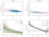 |
Fig. 2. Correlation between the turnaround density offset of a structure and the deviations of its neighbours from spherical symmetry. Upper panel: blue points show the turnaround density offset ρta/ρta,SCM as a function of the sphericity metric α3D (see text) for MDPL2 and Virgo ΛSCDM halos at a redshift z = 0. The two quantities are negatively correlated, as is confirmed by a Spearman test: very significant (very low p-value) moderate correlation, with a correlation coefficient of −0.42 and −0.39 for the two simulations, respectively. The red line shows the mean value of the offset in bins of α3D. The error in the y-axis depicts the standard error of the mean. The lower panel shows the same as the red points in the upper panel. Different colors represent different redshifts in MDPL2 and Virgo ΛSCDM. In the case of MDPL2 (left panel), we also included a low-tone shaded region showing the 1σ spread of points around the mean. |
Even by inspection of this figure alone, it is clear that these two quantities are negatively correlated, as would intuitively be expected: the closer the dark matter halo distribution around a halo is to spherical symmetry, the smaller the offset of the turnaround density from the spherical collapse expectation. In order to make the trend even more apparent, we overplot in red the mean value of the offset for bins of the sphericity metric α3D. The offset plateaus at zero (the ratio of ρta over the spherical collapse prediction plateaus at 1) for α3D ≳ 0.6.
This correlation is robust with cosmic time, as is shown in the lower panel of Fig. 2, where we plot again the mean value of the offset in α3D bins for MDPL2 halos of various redshifts up to a redshift of z ∼ 1. Again, for α3D ≳ 0.6, the offset tends to scatter uniformly around zero. This trend holds for all cosmologies tested in this work.
3.3. Offset evolution is eliminated by sphericity cuts
We have established that the deviation of the ρta of a structure from the prediction of the SCM is strongly correlated with the deviation of the distribution of its neighbors from spherical symmetry and that, importantly, this correlation remains robust up to a redshift of one. Hence, we hypothesize that we can use α3D as a selection criterion to eliminate the offset that plagues the measurement of the turnaround density. That is, if we were to impose a cut in our analysis and examine halos with α3D ≥ 0.5, we might be able to cause the offset to disappear.
The implementation of this cut is shown in Fig. 3, where as in the upper panel of Fig. 1, we plot the evolution Ωta with redshift for halos from the Virgo simulations. When compared with Fig. 1, it is clear that the offset has been essentially eliminated at all redshifts. Importantly, simulations with almost identical cosmologies (MDPL2 and Virgo ΛCDM) but very different offset behaviors yield practically identical results after the implementation of this same single quality cut (see the blue and black points in Fig. 3). We can thus conclude that the asphericity hypothesis provides a unified cosmology-independent explanation for the origin of the offset.
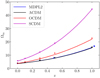 |
Fig. 3. As in the upper panel of Fig. 1, we plot the evolution Ωta with redshift and compare it to the prediction of the SCM for the Virgo simulations and for halos with α3D ≥ 0.5. With this cutoff, the offset between the points and solid lines is practically entirely eliminated. |
With the offset eliminated, the properties of the ρta(z) as a cosmology probe, as discussed in Pavlidou et al. (2020) using the SCM, now emerge in the simulation results as well: A measurement of ρta in a sample of sufficiently spherical halos at a single redshift (z = 0) informs us of the value of the dark matter density in the universe. A few such measurements at higher z (up to a z = 0.5) are sufficient to distinguish between universes with the same dark matter content, but a different cosmological constant.
4. Conclusions
This work is a follow-up to Korkidis et al. (2020), where we used N-body simulations for three different cosmologies to measure the turnaround density of cluster-sized halos in different redshifts, compared it to the predictions of the spherical-collapse model, and addressed the deviations between spherical collapse and simulations in different cosmologies. Specifically, we tested ΛSCDM, OCDM, and SCDM simulations, and analyzed snapshots of these at various z ≤ 1.
We found that the halo dark matter density at the turnaround approximately agrees with the prediction of the spherical collapse model for all cosmologies. However, we detected an offset between ρta in simulations and SCM that evolves (decreases) with redshift. We found that the offset is strongly anti-correlated with the degree of spherical symmetry in the distribution of neighbors. By applying quality cuts to the sample of simulated clusters for which we measured ρta, and in particular, by excluding halos whose distribution of massive neighbors was too aspherical, we eliminated (on average) this offset for all cosmologies and all redshifts. Because this selection criterion is independent of cosmology and redshift, its use restores the potential of ρta as a potential cosmological observable.
Nboykit is a massively parallel large-scale structure toolkit in python. For more details:
This redshift range is more than adequate: in Pavlidou et al. (2020), we explicitly showed that in the context of the spherical-collapse model, by measuring ρta and its evolution with cosmic time, we can distinguish between different cosmological models by a redshift z = 0.3 if observations of thousands of clusters are available at that z and they do not suffer from any offset.
Acknowledgments
We acknowledge support by the Hellenic Foundation for Research and Innovation under the “First Call for H.F.R.I. Research Projects to support Faculty members and Researchers and the procurement of high-cost research equipment grant”, Project 1552 CIRCE (GK, VP); by the European Research Council under the European Union’s Horizon 2020 research and innovation programme, grant agreement No. 771282 (KT); and by the Foundation of Research and Technology – Hellas Synergy Grants Program (project MagMASim, VP, and project POLAR, KT). The CosmoSim database used in this paper is a service by the Leibniz-Institute for Astrophysics Potsdam (AIP). The MultiDark database was developed in cooperation with the Spanish MultiDark Consolider Project CSD2009-00064. The authors gratefully acknowledge the Gauss Centre for Supercomputing e.V. (https://www.gauss-centre.eu) and the Partnership for Advanced Supercomputing in Europe (PRACE, https://www.prace-ri.eu) for funding the MultiDark simulation project by providing computing time on the GCS Supercomputer SuperMUC at Leibniz Supercomputing Centre (LRZ, https://www.lrz.de). The Bolshoi simulations have been performed within the Bolshoi project of the University of California High-Performance AstroComputing Center (UC-HiPACC) and were run at the NASA Ames Research Center. The simulations in this paper were carried out by the Virgo Supercomputing Consortium using computers based at Computing Centre of the Max-Planck Society in Garching and at the Edinburgh Parallel Computing Centre. The data are publicly available at https://www.mpa-garching.mpg.de/galform/virgo/int_sims Throughout this work we relied extensively on the PYTHON packages Numpy (Harris et al. 2020), Scipy (Virtanen et al. 2020) and Matplotlib (Hunter 2007).
References
- Adhikari, S., Dalal, N., & Chamberlain, R. T. 2014, JCAP, 2014, 019 [Google Scholar]
- Behroozi, P. S., Wechsler, R. H., & Wu, H.-Y. 2013, ApJ, 762, 109 [NASA ADS] [CrossRef] [Google Scholar]
- Bertschinger, E. 1985, ApJS, 58, 39 [Google Scholar]
- Busha, M. T., Evrard, A. E., Adams, F. C., & Wechsler, R. H. 2005, MNRAS, 363, L11 [NASA ADS] [Google Scholar]
- Capozziello, S., Dialektopoulos, K. F., & Luongo, O. 2019, Int. J. Mod. Phys. D, 28, 1950058 [NASA ADS] [CrossRef] [Google Scholar]
- Cuesta, A. J., Prada, F., Klypin, A., & Moles, M. 2008, MNRAS, 389, 385 [NASA ADS] [CrossRef] [Google Scholar]
- Cupani, G., Mezzetti, M., & Mardirossian, F. 2008, MNRAS, 390, 645 [NASA ADS] [CrossRef] [Google Scholar]
- Davis, M., Efstathiou, G., Frenk, C. S., & White, S. D. M. 1985, ApJ, 292, 371 [Google Scholar]
- Del Popolo, A. 2020, Astron. Rep., 64, 641 [Google Scholar]
- Diemer, B., & Kravtsov, A. V. 2014, ApJ, 789, 1 [NASA ADS] [CrossRef] [Google Scholar]
- Faraoni, V., Giusti, A., & Côté, J. 2020, Phys. Rev. D, 102, 044002 [NASA ADS] [CrossRef] [Google Scholar]
- Fillmore, J. A., & Goldreich, P. 1984, ApJ, 281, 1 [Google Scholar]
- Gunn, J. E. 1977, ApJ, 218, 592 [NASA ADS] [CrossRef] [Google Scholar]
- Gunn, J. E., Gott, J., & Richard, I. 1972, ApJ, 176, 1 [Google Scholar]
- Harris, C. R., Millman, K. J., van der Walt, S. J., et al. 2020, Nature, 585, 357 [NASA ADS] [CrossRef] [Google Scholar]
- Hunter, J. D. 2007, Comput. Sci. Eng., 9, 90 [NASA ADS] [CrossRef] [Google Scholar]
- Klypin, A., Yepes, G., Gottlöber, S., Prada, F., & Heß, S. 2016, MNRAS, 457, 4340 [Google Scholar]
- Korkidis, G., Pavlidou, V., Tassis, K., et al. 2020, A&A, 639, A122 [EDP Sciences] [Google Scholar]
- Lahav, O., Lilje, P. B., Primack, J. R., & Rees, M. J. 1991, MNRAS, 251, 128 [Google Scholar]
- Lee, J., & Baldi, M. 2022, ApJ, 938, 137 [NASA ADS] [CrossRef] [Google Scholar]
- Lopes, R. C. C., Voivodic, R., Abramo, L. R., & Sodré, L. J. 2019, JCAP, 2019, 026 [CrossRef] [Google Scholar]
- More, S., Diemer, B., & Kravtsov, A. V. 2015, ApJ, 810, 36 [Google Scholar]
- Nojiri, S., Odintsov, S. D., & Faraoni, V. 2018, Phys. Rev. D, 98, 024005 [NASA ADS] [CrossRef] [Google Scholar]
- Pavlidou, V., & Tomaras, T. N. 2014, JCAP, 9, 020 [Google Scholar]
- Pavlidou, V., Korkidis, G., Tomaras, T. N., & Tanoglidis, D. 2020, A&A, 638, L8 [NASA ADS] [CrossRef] [EDP Sciences] [Google Scholar]
- Planck Collaboration XIII. 2016, A&A, 594, A13 [NASA ADS] [CrossRef] [EDP Sciences] [Google Scholar]
- Santa Vélez, C., & Enea Romano, A. 2020, JCAP, 2020, 022 [CrossRef] [Google Scholar]
- Tanoglidis, D., Pavlidou, V., & Tomaras, T. N. 2015, JCAP, 2015, 060 [CrossRef] [Google Scholar]
- Tanoglidis, D., Pavlidou, V., & Tomaras, T. 2016, arXiv e-prints [arXiv:1601.03740] [Google Scholar]
- Virtanen, P., Gommers, R., Oliphant, T. E., et al. 2020, Nat. Methods, 17, 261 [Google Scholar]
- Vogelsberger, M., & White, S. D. M. 2011, MNRAS, 413, 1419 [NASA ADS] [CrossRef] [Google Scholar]
- Wong, C. C. 2019, arXiv e-prints [arXiv:1910.10477] [Google Scholar]
Appendix A: Full correlations of turnaround mass and turnaround radius
In Korkidis et al. (2020), the turnaround radius and mass were shown to scale as ( ) so that a characteristic density on the turnaround scale of a structure can be defined. In this appendix, we verify that this remains true across redshifts in all simulations and cosmologies considered here. Figure A.1 shows the quantity
  plotted against the turnaround mass Mta for all simulations considered in this work, and for all the redshift snapshots we analyzed. Rta is the kinematically defined turnaround radius, and ρSCM is the spherical-collapse model prediction for the turnaround density for the corresponding redshift and cosmology. For halos that behave exactly as the spherical collapse prediction, points should fall exactly on the y = x line, which we overplot as the solid blue line. The left panel shows all halos in each snapshot, and the right panel only shows the least aspherical halos (α3D ≥ 0.6, see Sect. 3.2).
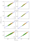 |
Fig. A.1. Correlation of the turnaround mass and turnaround radius. Different colors and symbols represent different redshifts. Different rows depict different simulated cosmologies, as in the titles. In order to have the same scale for different redshifts, the third power of the turnaround radius was multiplied by the spherical-collapse–predicted turnaround density for the given cosmology and redshift. The right panel in each row shows the least-aspherical subsample of the structures (α3D ≥ 0.6; see Sect. 3.2). The blue line represents the y = x line. |
All Tables
All Figures
|
Fig. 1. Evolution of the turnaround density with redshift. Upper panel: data points: Ωta vs. redshift for the three Virgo cosmologies [ΛSCDM (black points), OCDM (red points), and SCDM (magenta points)] and for the MDPL2 ΛSCDM run. Each point corresponds to the mean value of Ωta in the halo sample at that z, and the error bars (in most cases smaller than the symbol size) correspond to the standard error on the mean. Solid lines: spherical-collapse prediction for Ωta vs. z for the corresponding cosmology. Lower panel: ratio of Ωta in simulations over the spherical-collapse prediction as a function of z for the Virgo and MDPL2 simulations. There is a small, evolving offset between the kinematically measured turnaround density in simulated halos and the spherical-collapse prediction. |
| In the text | |
|
Fig. 2. Correlation between the turnaround density offset of a structure and the deviations of its neighbours from spherical symmetry. Upper panel: blue points show the turnaround density offset ρta/ρta,SCM as a function of the sphericity metric α3D (see text) for MDPL2 and Virgo ΛSCDM halos at a redshift z = 0. The two quantities are negatively correlated, as is confirmed by a Spearman test: very significant (very low p-value) moderate correlation, with a correlation coefficient of −0.42 and −0.39 for the two simulations, respectively. The red line shows the mean value of the offset in bins of α3D. The error in the y-axis depicts the standard error of the mean. The lower panel shows the same as the red points in the upper panel. Different colors represent different redshifts in MDPL2 and Virgo ΛSCDM. In the case of MDPL2 (left panel), we also included a low-tone shaded region showing the 1σ spread of points around the mean. |
| In the text | |
|
Fig. 3. As in the upper panel of Fig. 1, we plot the evolution Ωta with redshift and compare it to the prediction of the SCM for the Virgo simulations and for halos with α3D ≥ 0.5. With this cutoff, the offset between the points and solid lines is practically entirely eliminated. |
| In the text | |
|
Fig. A.1. Correlation of the turnaround mass and turnaround radius. Different colors and symbols represent different redshifts. Different rows depict different simulated cosmologies, as in the titles. In order to have the same scale for different redshifts, the third power of the turnaround radius was multiplied by the spherical-collapse–predicted turnaround density for the given cosmology and redshift. The right panel in each row shows the least-aspherical subsample of the structures (α3D ≥ 0.6; see Sect. 3.2). The blue line represents the y = x line. |
| In the text | |
Current usage metrics show cumulative count of Article Views (full-text article views including HTML views, PDF and ePub downloads, according to the available data) and Abstracts Views on Vision4Press platform.
Data correspond to usage on the plateform after 2015. The current usage metrics is available 48-96 hours after online publication and is updated daily on week days.
Initial download of the metrics may take a while.