| Issue |
A&A
Volume 672, April 2023
|
|
|---|---|---|
| Article Number | A105 | |
| Number of page(s) | 8 | |
| Section | The Sun and the Heliosphere | |
| DOI | https://doi.org/10.1051/0004-6361/202245049 | |
| Published online | 06 April 2023 | |
Cutoff of transverse waves through the solar transition region
1
Université Paris-Saclay, CNRS, Institut d’Astrophysique Spatiale, 91405 Orsay, France
2
Centre for mathematical Plasma Astrophysics, Department of Mathematics, KU Leuven, Celestijnenlaan 200B, 3001 Leuven, Belgium
e-mail: This email address is being protected from spambots. You need JavaScript enabled to view it.
3
Department of Mathematics, Physics and Electrical Engineering, Northumbria University, Newcastle upon Tyne NE1 8ST, UK
Received:
23
September
2022
Accepted:
3
January
2023
Abstract
Context. Transverse oscillations are ubiquitously observed in the solar corona, both in coronal loops and in open magnetic flux tubes. Numerical simulations suggest that their dissipation could heat coronal loops, thus counterbalancing radiative losses. These models rely on a continuous driver at the footpoint of the loops. However, analytical works predict that transverse waves are subject to a cutoff in the transition region. It is thus unclear whether they can reach the corona and indeed heat coronal loops.
Aims. Our aims are to determine how the cutoff of kink waves affects their propagation into the corona and to characterize the variation of the cutoff frequency with altitude.
Methods. Using 3D magnetohydrodynamic simulations, we modelled the propagation of kink waves in a magnetic flux tube, embedded in a realistic atmosphere with thermal conduction, which starts in the chromosphere and extends into the corona. We drove kink waves at four different frequencies and determined whether they experienced a cutoff. We then calculated the altitude at which the waves were cut off and compared it to the prediction of several analytical models.
Results. We show that kink waves indeed experience a cutoff in the transition region, and we identified the analytical model that gives the best predictions. In addition, we show that waves with periods shorter than approximately 500 s can still reach the corona by tunnelling through the transition region with little to no attenuation of their amplitude. This means that such waves can still propagate from the footpoints of loop and result in heating in the corona.
Key words: Sun: atmosphere / Sun: oscillations / magnetohydrodynamics (MHD) / waves / methods: numerical
© The Authors 2023
 Open Access article, published by EDP Sciences, under the terms of the Creative Commons Attribution License (https://creativecommons.org/licenses/by/4.0), which permits unrestricted use, distribution, and reproduction in any medium, provided the original work is properly cited.
This article is published in open access under the Subscribe to Open model. This email address is being protected from spambots. You need JavaScript enabled to view it. to support open access publication.
1. Introduction
Recent advances in observations and modelling have shown that magnetohydrodynamic (MHD) waves could significantly contribute to the heating of the solar corona (see review by Van Doorsselaere et al. 2020). In particular, transverse waves are ubiquitously observed, and several kinds have been identified. The type that was first discovered are the transverse waves that are impulsively excited after a flare (Nakariakov et al. 1999). However, these transverse waves are only sporadically excited and do not play an important role in the energy budget of the solar corona (Terradas & Arregui 2018). Later on it was discovered that the corona is filled by small-amplitude transverse waves (Tomczyk et al. 2007; Tomczyk & McIntosh 2009; McIntosh et al. 2011; Tian et al. 2012). These were observed in coronal loops as propagating (Tiwari et al. 2019) or standing waves (Anfinogentov et al. 2015). These low-amplitude transverse waves were also observed as propagating waves in open-field regions (Thurgood et al. 2014; Morton et al. 2015). These low-amplitude waves show little to no decay (Morton et al. 2021), and are thus named ‘decayless’.
Because the flare-excited standing waves rapidly decay (Goddard et al. 2016; Nechaeva et al. 2019) due to resonant absorption (Goossens et al. 2002) and non-linear Kelvin–Helmholtz instability (KHI) damping (Terradas et al. 2008; Antolin et al. 2014; Van Doorsselaere et al. 2021; Arregui 2021), it is generally thought that the decayless waves must be continuously supplied with energy to counteract the strong damping. Several mechanisms for excitation have been proposed: slip-stick driving with steady flows (Nakariakov et al. 2016; Karampelas & Van Doorsselaere 2020), vortex shedding (Nakariakov et al. 2009; Karampelas & Van Doorsselaere 2021), and footpoint driving (Nisticò et al. 2013; Karampelas et al. 2017) through p-modes (Morton et al. 2019) or convective shuffling. The option of footpoint driving has had some success in generating standing mode decayless waves (Afanasyev et al. 2020), which counterbalance the non-linear damping through the KHI (Guo et al. 2019) and heat the loops (Shi et al. 2021).
However, for the driving of decayless waves through their footpoints, it is not well understood how the transverse waves propagate through the complicated structure of the chromosphere and transition region. The simulations of transverse-wave-induced KHI heating (e.g., Karampelas et al. 2019) only take into account the coronal part of the loop; in other words, a driver is imposed at the top of the transition region. To properly model the whole loop evolution due to the wave heating, it is essential to also model the wave driver in the photosphere and accurately capture its influence on the coronal loop dynamics.
In plane-parallel atmospheres the propagation of fast and slow waves has been well studied. It was found that these modes couple efficiently to Alfvén waves through resonant absorption (Hansen & Cally 2009; Cally & Andries 2010; Khomenko & Cally 2012). Currently, investigations into what happens if the cross-field structuring is included in the wave propagation model are ongoing (Cally & Khomenko 2019; Riedl et al. 2019, 2021). Another crucial ingredient is the wave’s behaviour in strong (i.e., non-Wentzel-Kramers-Brillouin, non-WKB) stratification. It is well known that slow waves experience a cutoff while propagating through a stratified medium (Bel & Leroy 1977). This has been verified observationally (Jess et al. 2013) and numerically (Felipe et al. 2018), although it is still unknown whether a similar cutoff exists for transverse waves in structured media. For the driving of the observed decayless waves in the corona, this is a crucial property to understand.
Several analytical works predict that transverse waves are cut off in the transition below a given frequency. The first formula was derived by Spruit (1981):
 (1)
(1)
Here g is the gravity projected along the loop, H the pressure scale height, and β the ratio of the gas to the magnetic pressures. For a typical isothermal atmosphere, this corresponds to a cutoff period of 700 s (Spruit 1981). However, Lopin et al. (2014) showed that this classical cutoff is suppressed when the radial component of the magnetic field is taken into account. Lopin & Nagorny (2017) later showed that transverse waves can still be cut off, provided a non-isothermal atmosphere. They predict a cutoff frequency of
 (2)
(2)
where z is the altitude, ck0 is the kink speed at the base of atmosphere (z = z0), H is the pressure scale height, H0 = H(z0), and  is the relative difference between the magnetic field inside (B0, i) and outside (B0, e) the flux tube at z = z0. Finally, an alternative formula was derived by Snow et al. (2017),
 (3)
(3)
where z is the altitude and vA is the Alfvén speed.
In this article we modelled the propagation of kink waves in an open magnetic flux tube, embedded in a non-isothermal atmosphere. The atmosphere extends from the chromosphere to the corona, and includes gravitational stratification and thermal conduction (Sect. 2). We drove kink waves at different periods, and determined whether they experienced a cutoff (Sect. 3). We compare these results to the three analytical formulas given above in Sect. 4, and summarize our conclusions in Sect. 5.
2. Numerical model: Magnetic flux tube through the transition region
We modelled a vertical magnetic flux tube of radius R = 1 Mm embedded in a stratified atmosphere, starting in the chromosphere (altitude z = 0 Mm) and extending through the transition region (z ≈ 4 Mm) into the corona. Kink waves were excited in the flux tube by applying a monoperiodic driver at the bottom of the domain (z = 0 Mm). In the upper half of the domain (z > 50 Mm), we implemented a ‘velocity rewrite layer’ to absorb the kink waves. The driver and the velocity rewrite layer are described in Sect. 2.1. A sketch of the domain is shown in Fig. 1. We solved the 3D MHD evolution of this tube using the PLUTO code (Mignone et al. 2007), version 4.3. This code solves the conservative MHD equations (mass continuity, momentum conservation, energy conservation, and induction equation). We used the corner transport upwind finite volume scheme, where characteristic tracing is used for the time stepping and a linear spatial reconstruction with a monotonized central difference limiter is performed. The magnetic field divergence was kept small using the extended divergence cleaning method (generalized Lagrange multiplier, or GLM), and the flux was computed with the linearized Roe Riemann solver. We did not include explicit viscosity, resistivity, or cooling. However, numerical dissipation results in higher effective viscosity and resistivity than expected for the solar corona, as discussed by Karampelas et al. (2019). We included a modified thermal conduction, as described below.
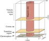 |
Fig. 1. Sketch of the simulation domain, showing the magnetic flux tube, the location of the kink wave driver (bottom boundary), chromosphere, transition region, corona, and velocity rewrite layer. |
The transition region between the chromosphere and the corona is characterized by a very sharp temperature gradient. Resolving this gradient requires a very high resolution along the tube (∼1 km in the transition region). In order to keep computational costs reasonable, we artificially broadened the transition region (thus reducing the temperature gradient). To that end, we modified the thermal conductivity using the method developed by Linker et al. (2001), Lionello et al. (2009), and Mikić et al. (2013). Below the cutoff temperature Tc = 2.5 × 10⁵ K, the parallel thermal conductivity was set to  with C0 = 9 × 10⁻¹² W m−1 K−7/2; above Tc, it was set to κ∥ = C0T5/2. This allowed us to use a resolution of 98 km along the tube. This grid allows us to fully resolve the broadened transition region, which has a minimum temperature scale length of 1.6 Mm (see Johnston & Bradshaw 2019). The dimensions of the domain were (Lx, Ly, Lz) = (16, 6, 100) Mm. We used a uniform grid of 400 × 150 × 1024 cells, with a size of 40 km in the x and y directions, and 98 km in the z direction. Furthermore, we verified that the results did not change significantly when using a resolution of 40 km in the z direction. To that end, we ran a separate simulation and verified that the resulting cutoff altitude and comparison to the analytical formulas (see Sect. 4) were not strongly modified. We note that this resolution is too costly in terms of running time to be used for all simulations in this work.
The strong stratification in the transition region makes it challenging to obtain a relaxed initial state for the model. We first initialized the domain with a field-aligned hydrostatic equilibrium (Sect. 2.2). We then let the simulation relax in 2D for 47 ks (Sect. 2.3). Finally, we filled the 3D domain with this relaxed state through cylindrical symmetry, where we drove kink waves of different periods for a duration up to 2.7 ks (Sect. 2.4).
2.1. Boundary conditions and driver
We first describe the boundary conditions used for the relaxation (2D) and kink wave (3D) simulations.
Bottom boundary. At the bottom boundary (base of the chromosphere, z = 0), the density and pressure were extrapolated using the hydrostatic equilibrium equation. The magnetic field was extrapolated using the zero normal-gradient condition described by Karampelas et al. (2019, Sect. 2.4). For vz, we either imposed a reflective boundary condition (2D relaxation, see Sect. 2.3), or imposed vz = 0 (in 3D, see Sect. 2.4). We verified that both boundary conditions give the same results in 3D simulations. The parallel velocity components vx and vy were set to obey either a zero-gradient boundary condition (2D relaxation), or to follow a driver that excites kink waves (in 3D). We used a monoperiodic, dipole-like, driver developed by Pascoe et al. (2010) and updated by Karampelas et al. (2017). Inside the tube the driver imposes
 (4)
(4)
where v(t) = v0cos(2πt/P0), with v0 the driver amplitude set to 2 km s−1. The driver period, P0, was set to different values in order to test the cut off of kink waves. Outside the tube the driver imposes
 (5)
(5)
where x0(t) = v0P0/(2π)⋅sin(2πt/P0) is the centre of the tube’s footpoint at time t. This driver generates a kink wave polarized in the x direction.
Upper boundary. At the upper boundary (top of the corona, z = 100 Mm), the magnetic field was kept symmetric. All other variables obeyed a reflective boundary condition. In order to absorb the upward waves excited by the driver, we artificially modified the velocity in the upper half of the domain (z > 50 Mm). At each time step, after solving the MHD equations, we decreased each component of the velocity vi by multiplying it by a quantity αv ≲ 1:
 (6)
(6)
In the driven 3D simulations αv was kept constant in time and varied linearly along the loop, from 1 at z = zv = 50 Mm to αv,min = 0.9995 at z = L = 100 Mm:
 (7)
(7)
In the 2D relaxation run, the first third of the simulation (t1/3 = 15.7 ks) was run without modifying the velocity (i.e., αv = 1). During the second third αv was linearly ramped down in time to match the profile αv, 3D(z) described above. Finally, the last third of the simulation was run with the constant αv, 3D(z):
 (8)
(8)
The evolution of αv is shown in Fig. 2. This velocity rewrite layer can successfully absorb the kink waves that are excited by the driver at the bottom of the chromosphere. As a result, these waves are not reflected at the upper boundary, and do not propagate downwards back into the domain. We note that the solution obtained inside the velocity rewrite layer (i.e., above z = 50 Mm) is not physical, and that this layer should be considered a part of the upper boundary.
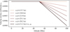 |
Fig. 2. Velocity-rewrite coefficient αv, applied to the velocity above 50 Mm so that upper-propagating waves are not reflected back into the domain. αv is shown for different times of the 2D relaxation run. The last profile (t ≥ 31.3 ks) is also applied in the 3D driven simulations. |
Side boundaries. At the side boundaries (x and y axes), all variables obeyed a zero-gradient boundary condition. In the 2D relaxation run, we only simulated half of the tube radius (x > 0). For these simulations, we imposed a reflective boundary condition on all variables at the centre of the tube (x = 0).
2.2. Initial conditions: Field-aligned hydrostatic equilibrium
The simulation was initialized with a uniform vertical magnetic field of magnitude B0 = 42 G. Along the tube, we imposed the temperature profile derived from Aschwanden & Schrijver (2002)
 (9)
(9)
where z is the altitude, L is the height of the computational domain, Δch = 4 Mm is thickness of the chromosphere, and Tch = 20 000 K is the temperature in the chromosphere. We defined the transverse temperature profile at the top of the domain, Tcor(x, y), as
 (10)
(10)
where Tcor, int = 1.2 MK is the temperature inside the tube, and Tcor, ext = 3.6 MK is the temperature outside the tube. The shape of the profile was set by ζ(x, y),
![Mathematical equation: $$ \begin{aligned} \zeta (x, y) = \frac{1}{2} \left[ 1 - \tanh \left( \left( \sqrt{x^2 + y^2} / R - 1 \right) b \right) \right], \end{aligned} $$](/articles/aa/full_html/2023/04/aa45049-22/aa45049-22-eq13.gif) (11)
(11)
where R = 1 Mm is the tube radius and b = 5 is a dimensionless number setting the width of the inhomogeneous layer between the interior and exterior of the tube (l ≈ 6R/b). The value of ζ(x, y) is close to 1 inside the tube, and to 0 outside.
We also set the density at the bottom of the chromosphere (z = 0) to
 (12)
(12)
where ρch, int = 3.51 × 10⁻⁸ kg m−3 is the density inside the tube and ρch, ext = 1.17 × 10⁻⁸ kg m−3 is the density outside. We then integrated the field-aligned hydrostatic equilibrium equation numerically using a Crank–Nicholson scheme. The profiles of the imposed temperature and of the density resulting from the integration are shown in Fig. 3a. The temperature contrast (interior temperature divided by exterior temperature) is 1 in the chromosphere, and decreases to 1/3 in the corona. The density contrast is 3 in the chromosphere, increases to around 7 in the transition region, and decreases again to about 4 in the upper corona. The pressure contrast is 3 in the chromosphere, and slowly decreases to reach 1.2 in the upper corona.
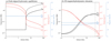 |
Fig. 3. Temperature (black), density (red), and magnetic field magnitude (blue) profiles inside (r = 0 Mm; solid lines) and outside (r = 8 Mm; dashed lines) the flux tube. (a) After solving the field-aligned hydrostatic equilibrium. (b) After the 2D magnetohydrodynamic relaxation. |
However, this initial state is not in magnetohydrostatic (MHS) equilibrium because the pressure varies across the flux tube, while the magnetic field does not. To fix this, we let the tube relax by running a 2D magnetohydrodynamic simulation (Sect. 2.3). We then used this relaxed state to initialize the 3D simulation of kink waves (Sect. 2.4).
2.3. Flux tube relaxation (2D)
In order to obtain a flux tube in MHS equilibrium, we first ran a 2D simulation, initialized with the initial state described in Sect. 2.2. The MHD equations were solved in a longitudinal plane at y = 0 (see Fig. 1), with x ∈ [0, 8.56] Mm and z ∈ [0, 100] Mm. We used a uniform grid of 64 × 2048 cells with a size of 134 km × 49 km. The resolution along z was higher than in the 3D runs in order to resolve the sharper gradients in the transition region (see Fig. 3). We verified that a resolution of 40 km in the x direction yielded the same results by running a separate 2D simulation followed by a 3D driven simulation (P0 = 200 s), and verifying that the cutoff altitude and comparison to the analytical formulas (Sect. 4) were not significantly modified.
We let the system evolve for 47 ks, during which the velocity rewrite parameter αv varied as described in Eq. (8). As a result of the relaxation, periodic longitudinal flows with a velocity of about 15 km s−1 develop along the tube. They are damped during the later stages of the simulation, as the velocity rewrite layer is gradually introduced. At the end of the relaxation run, residual velocities are lower than 0.5 km s−1 everywhere in the domain. The resulting temperature, density, and magnetic field profiles are shown in Fig. 3b. Compared to the initial state (Fig. 3a), the transition region is significantly broadened, with a thickness of about 7 Mm. This is the direct result of the modified thermal conductivity used in this set-up, and allows for a coarser resolution along the loop in the 3D simulations. In addition, the temperature and density decrease, both inside and outside the tube. Overall, the density contrast (ρint/ρext) decreases: it reaches 1 in the chromosphere, 1.2 in the transition region, and 1.8 in the corona. The temperature contrast also changes to about 1.3 in the transition and about 0.8 in the corona. Finally, the magnetic field amplitude contrast remains very close to 1 everywhere in the domain (0.97 in the chromosphere and 1 in the corona), with a magnitude of about 11 G everywhere in the domain. Compared to the initial uniform magnetic field, the magnitude is divided by about four, while the contrast remains close to 1. The final temperature and density profile significantly differ from the initial conditions of the 2D relaxation run. However, this is not an issue as the goal of this study is to investigate how the analytical formulas we consider (Spruit 1981; Lopin & Nagorny 2017; Snow et al. 2017) predict the cutoff frequency for a given temperature and density profile. By using the relaxed profiles as input to these analytical formulas, we obtained predictions for the relaxed system.
This relaxed 2D simulation was then mapped onto the 3D domain through cylindrical symmetry. We used a rotation about the line x = 0 (i.e., the centre of the loop), and a trilinear interpolation to project onto the 3D Cartesian grid.
2.4. Kink wave propagation (3D)
In order to simulate the propagation of kink waves from the chromosphere to the corona, we drove the 3D simulations with the monoperiodic, dipole-like, driver described in Eqs. (4) and (5). We ran four simulations, with different driver periods P0: 200 s, 335 s, 700 s, and 2000 s. The propagating kink waves generated by the driver are absorbed by the velocity rewrite layer at the top of the domain, and are thus not reflected downwards. The first three simulations were run for a duration of 5P0. The last simulation was run for 1.75P0. At the beginning of the simulations, the system goes through an initial transitory phase before the propagating kink wave is fully established (i.e. its amplitude does not change with time). We waited for 2P0 (0.42P0 for P0 = 2000 s) for the kink wave to enter a stable sinusoidal regime. After this duration we saved high-cadence snapshots at the centre of the loop (line x = y = 0). For all further analyses we used the snapshots saved after the transitory phase. The transverse velocity vx at the loop centre is shown in Fig. 4. As can be seen in this figure, the amplitude of the kink wave decreases as the period increases. For the two longer driver periods (700 and 2000 s), the amplitude of the kink wave is small enough for some perturbations to become visible. They travel at the Alfvén speed, and appear to be triggered by the flows remaining after the relaxation (see Sect. 2.3). These perturbations have amplitudes smaller than 0.2 km s−1, and should thus have no effect on the wave.
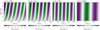 |
Fig. 4. Kink wave transverse velocity (vx) at the loop centre (x = y = 0) as a function of altitude and time. The velocity is shown for four 3D simulations with different driver periods P0, after an initial settling time of 2P0 (for P0 = 200 s, 335 s, and 700 s), or 0.42P0 (for P0 = 2000 s). The dashed black lines represent a propagation at the kink speed (see Eq. (13)), and are independent of the driver period. |
3. Results: Cut off and tunnelling of transverse waves
In order to determine whether the kink waves driven in the 3D simulations are experiencing a cut off, we looked at the evolution of the velocity amplitude (Sect. 3.1), as well as the phase speed (Sect. 3.2) as a function of altitude. The analysis of these profiles allows us to establish that the transverse waves are subject to a low-frequency cutoff in the transition region.
3.1. Wave amplitude increases with frequency
In order to compute the velocity amplitude of the kink wave, we fitted the function Ax(z)sin(ω(z)t+ϕ(z)) to the transverse velocity vx(z, t), at each altitude (z). Here Ax(z) is the velocity amplitude, ω(z) is the kink wave frequency, and ϕ(z) is the phase. The frequency varies by less than 1% with altitude, confirming the theoretical understanding. The velocity amplitude is shown in Fig. 5. In all simulations, the wave amplitude increases with altitude because of the density decreases with altitude and energy conservation. Across the simulations the amplitude at a given altitude increases with the frequency of the wave. This means that kink waves with higher frequencies propagate better from the chromosphere to the corona. This would be consistent with the low-frequency cutoff predicted by analytical models (see Sect. 1).
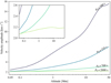 |
Fig. 5. Velocity amplitude of kink waves as a function of altitude. The velocity is shown for four different driver periods (P0). The inset has the same axes as the main figure, with a zoom-in on the vertical axis. |
3.2. Evanescent waves in the transition region
To determine the altitude at which the waves are cut off, we compared their phase speed vp(z) to the kink speed of the flux tube ck(z). The inverse phase speed is equivalent to the phase difference Δϕ(z) between two altitudes separated by Δz: 1/vp(z) = Δϕ(z)/(ωΔz). The phase difference has been successfully used to determine the cutoff frequency of acoustic and slow-magnetosonic waves in observations (Centeno et al. 2006; Felipe et al. 2010; Krishna Prasad et al. 2017; Felipe et al. 2018), and in simulations (Felipe & Sangeetha 2020). In these articles the authors determine the phase speed for a wide range of frequencies, but at a limited number of altitude positions. In the present study, however, we could only examine four frequencies because of the high computational cost of a simulation. However, we computed the phase difference at all altitudes of the simulation domain. This allows us to determine the altitude at which the wave is cut off.
The phase speed at a given altitude z was computed from the transverse velocity in the cells above and below: vx(t, z + Δz/2) and vx(t, z − Δz/2), where Δz = 98 km is the cell size. We apodized these velocity time series with a Hann window, and computed the cross-correlation: C(τ, z) = vx(t, z + Δz/2)⋆vx(t, z − Δz/2). We then determined the time delay Δτ(z) by finding the maximum of C(τ, z). To that end, we fitted the function A + Bcos(ω(τ−Δτ)/δ) to C(τ, z) with τ ∈ [ − P0/4, +P0/4]. Finally, the phase difference was given by Δϕ(z) = ωΔτ(z), and the inverse phase speed by 1/vp(z) = Δτ(z)/Δz. The inverse phase speed is shown in Fig. 6 along with the inverse kink speed for the simulated flux tube. The kink speed ck is calculated using
 (13)
(13)
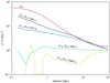 |
Fig. 6. Inverse phase speed of the kink wave (1/vp) and inverse kink speed of the flux tube (1/ck) as a function of altitude. The phase speed is given for four different driver periods (P0). |
where ρ(z) is the density,  is the Alfvén speed, B(z) is the magnetic field amplitude, and μ0 is the magnetic permittivity of vacuum. The indices i and e correspond, respectively, to internal and external quantities relative to the flux tube and are taken at x = 0 and x = 8 Mm.
In simulations with short driver periods, the inverse phase speed is somewhat smaller than the inverse kink speed in the chromosphere and transition region (vp/ck ≈ 2 for P0 = 200 s, and 5 for P0 = 335 s), and equals the inverse kink speed in the corona. On the other hand, in simulations with longer periods, the inverse phase speeds are much lower than the inverse kink speed below a given altitude. For P0 = 700 s, 1/vp is about 250 times smaller than 1/ck below z = 1 Mm. For P0 = 2000 s a similar drop occurs below z = 20 Mm.
For a propagating kink wave the inverse phase speed is expected to be equal to the inverse kink speed. Conversely, standing and evanescent (i.e., cutoff) waves have inverse phase speeds lower than the inverse kink speed. Thus, the decreased inverse phase speed for higher periods indicates that the waves are cut off in at least some regions.
To distinguish between the standing and evanescent cases, we also looked at the wave amplitude (Fig. 5). In the absence of vertical stratification, the amplitude of evanescent waves decreases with altitude. However, in a stratified atmosphere (our case), the amplitude increases with altitude because of the density decrease, even for evanescent waves. In Fig. 5, the amplitude of waves with longer periods (for which 1/vp ≪ 1/ck) increases less with altitude compared to waves with shorter periods (for which 1/vp ≲ 1/ck). We thus conclude that the waves with longer periods are evanescent in parts of the low atmosphere where their inverse phase speed is much lower than the inverse kink speed. This means that these long-period waves are cut off in the transition region.
3.3. Wave tunnelling at higher frequencies
Waves with shorter periods (P0 = 200 and 335 s) also show signs of cutoff at low altitudes. Below z = 3 Mm, the inverse phase speed 1/vp is lower than the inverse kink speed 1/ck (Fig. 6), and the amplitude increase with altitude is smaller for P0 = 335 s than for P0 = 200 s (Fig. 5). However, this cutoff is significantly weaker than in the long-period case. This is explained by the fact that the cutoff region (where 1/vp < 1/ck) is narrower for short periods (∼1 Mm) than for long periods (∼10 Mm). As a result, short-period waves can tunnel through the cutoff region, and propagate into the corona. Furthermore, the weak attenuation in the cutoff region results (1/vp ≲ 1/ck) further reduces the effect of the cutoff.
4. Discussion: Comparison to analytical formulas
In order to compare our simulations to the analytical models, we quantified the cutoff frequency as a function of altitude. We define zc, the altitude at which ck/vp goes above a given threshold tr. This corresponds to the altitude where the wave leaves the cutoff regime and enters the propagating regime (i.e., the cutoff altitude). We computed zc for four values of tr between 0.2 and 0.5. Considering the four simulations with different driver frequencies, ω, we obtained the cutoff altitude as a function of the frequency, zc(ω). We compare this to the cutoff frequency as a function of altitude, ωc(z), predicted by the analytical models presented in Sect. 1.
In Fig. 7 we show the cutoff frequency and altitude computed in our simulations, for different values of tr (black points). In the same figure we show the predictions of the analytical formulas of Spruit (1981, Eq. (1)), Lopin & Nagorny (2017, Eq. (2)), and Snow et al. (2017, Eq. (3)) (coloured lines) computed for the temperature and density profiles used in our simulations. We implement the formula of Lopin & Nagorny (2017) for different values of z0, defined by the authors as ‘the base of the atmosphere’, with no further details. Because this quantity is not accurately defined, we used four values of z0 in the range of 24 km (bottom cell of our simulation domain) to 1978 km. This loosely defined parameter broadens the range for the cutoff frequencies predicted by this formula. While the match is rather loose, the cutoff altitude zc(ω) measured in our simulations matches the overall variation the cutoff frequency ωc(z) predicted by the Lopin & Nagorny (2017) formula. In particular, the shape of the profiles are in good agreement. On the contrary, the Snow et al. (2017) model correctly predicts the cutoff frequency only in the lower transition region, but fails to do so in the upper transition region and corona. In particular, their model predicts a slower decrease in the cutoff frequency above 20 Mm, while the simulations and the Lopin & Nagorny (2017) formula show a continued decrease. Finally, the Spruit (1981) predictions are off by almost an order of magnitude at all altitudes. Thus, the formula of Lopin & Nagorny (2017) best predicts the cutoff frequency of transverse waves at different altitudes.
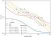 |
Fig. 7. Kink wave cutoff frequency as a function of altitude, from analytical models (see legend, left column) and from our numerical simulations (right column). We show the analytical predictions of Spruit (1981, SP81), Snow et al. (2017, Sn17), and Lopin & Nagorny (2017, LN17) (coloured lines). For the last model, we computed the cutoff frequency for different values of z0, the ‘base of the atmosphere’. We show the cutoff altitude (zc) for the four simulations that we ran with different driver frequencies (black symbols). The cutoff altitudes are computed with different thresholds tr, indicated in the legend and described in the text. |
While the broadened transition region in our simulations could affect the altitude-dependence of the cutoff frequency, this should have little impact on the validation of the analytical formulas. These formulas include the atmospheric stratification through altitude-dependent profiles of either the pressure scale height or the Alfvén speed (see Sect. 1). Because they make no hypothesis on these profiles, they should be valid regardless of the atmosphere considered. As such, the agreement with the simulations should not depend on the broadening of the transition region, provided the appropriate profile is fed into the formulas. After validating the Lopin & Nagorny (2017) formula by comparing it to our simulations, it should be applicable to other stratification profiles.
We note that while analytical formulas can predict the kink cutoff frequency, this is not sufficient to know whether a kink wave with a given frequency will propagate into the corona. To that end, the thickness of the cutoff region and the strength of the attenuation have to be taken into account. As shown by our simulations, kink waves with higher frequencies (≥3 mHz) can propagate into the corona by tunnelling through a region where they are cut off (Sect. 3.3). Furthermore, these waves only experience a weak attenuation because their frequency is close to the cutoff frequency. The cutoff frequency does not constitute a clear-cut boundary between oscillatory and non-oscillatory solutions. This was also reported for sound waves by Felipe & Sangeetha (2020). Although the question of whether a solution is oscillating is well defined mathematically, this is not straightforward to translate into a single cutoff frequency (Schmitz & Fleck 1998). For this reason there are several canonical definitions for cutoff frequencies, set within the continuous variation between the oscillating and non-oscillating regimes (see e.g., Schmitz & Fleck 1998 for sound waves in the solar atmosphere). As a result, cutoff frequencies are bound to be mere indications, rather than strong constraints on the physical behaviour of a wave (Chae & Litvinenko 2018).
5. Conclusions
Transverse waves are a candidate mechanism for heating the solar corona. However, several analytical models predicted that they are cut off in the transition region. In order to assess whether transverse waves can indeed heat the corona, it is thus crucial to determine whether they can propagate through the transition region. To that end, we have simulated the propagation of transverse kink waves in an open magnetic flux tube, embedded in an atmosphere extending from the chromosphere to the corona. We find that transverse waves are indeed cut off in the lower solar atmosphere. However, only waves with low frequencies (ν ≲ 2 mHz) are significantly affected. At higher frequencies, the cutoff occurs in a very thin layer (∼1 Mm), and results in a weak attenuation. In this case waves can tunnel through the cutoff layer, experiencing little to no amplitude attenuation. This means that transverse waves with high frequencies are able to transport energy from the chromosphere to the corona, where it can be dissipated and result in heating.
Furthermore, we compared our simulations to several analytical models that predict the cutoff frequency of transverse waves. We conclude that the formula proposed by Lopin & Nagorny (2017) gives the best prediction. While our simulations use a broadened transition, we expect it to have little impact on the validation of analytical formulas. As such, the formula by Lopin & Nagorny (2017) should be able to predict the cutoff frequency for any atmospheric stratification profile. We note that while the cutoff frequency is a good first indicator of whether a wave can propagate into the corona, it alone cannot predict the whole behaviour of the wave. In particular, waves with frequencies just below the cutoff frequency (which should thus be cut off) can still reach the corona thanks to a combination of tunnelling and weak attenuation.
Acknowledgments
This project has received funding from the European Research Council (ERC) under the European Union’s Horizon 2020 research and innovation program (grant agreement No. 724326). GP was supported by a CNES postdoctoral allocation. TVD was supported by the European Research Council (ERC) under the European Union’s Horizon 2020 research and innovation programme (grant agreement No 724326) and the C1 grant TRACEspace of Internal Funds KU Leuven. K.K. recognises support from a postdoctoral mandate from KU Leuven Internal Funds (PDM/2019), from a UK Science and Technology Facilities Council (STFC) grant ST/T000384/1, and from a FWO (Fonds voor Wetenschappelijk Onderzoek – Vlaanderen) postdoctoral fellowship (1273221N). The results received support from the FWO senior research project with number G088021N. Software: Astropy (Astropy Collaboration 2013, 2018).
References
- Afanasyev, A. N., Van Doorsselaere, T., & Nakariakov, V. M. 2020, A&A, 633, L8 [NASA ADS] [CrossRef] [EDP Sciences] [Google Scholar]
- Anfinogentov, S. A., Nakariakov, V. M., & Nisticò, G. 2015, A&A, 583, A136 [NASA ADS] [CrossRef] [EDP Sciences] [Google Scholar]
- Antolin, P., Yokoyama, T., & Van Doorsselaere, T. 2014, ApJ, 787, L22 [Google Scholar]
- Arregui, I. 2021, ApJ, 915, L25 [NASA ADS] [CrossRef] [Google Scholar]
- Aschwanden, M. J., & Schrijver, C. J. 2002, ApJS, 142, 269 [NASA ADS] [CrossRef] [Google Scholar]
- Astropy Collaboration (Robitaille, T. P., et al.) 2013, A&A, 558, A33 [NASA ADS] [CrossRef] [EDP Sciences] [Google Scholar]
- Astropy Collaboration (Price-Whelan, A. M., et al.) 2018, AJ, 156, 123 [Google Scholar]
- Bel, N., & Leroy, B. 1977, A&A, 55, 239 [NASA ADS] [Google Scholar]
- Cally, P. S., & Andries, J. 2010, Sol. Phys., 266, 17 [NASA ADS] [CrossRef] [Google Scholar]
- Cally, P. S., & Khomenko, E. 2019, ApJ, 885, 58 [Google Scholar]
- Centeno, R., Collados, M., & Trujillo Bueno, J. 2006, ApJ, 640, 1153 [Google Scholar]
- Chae, J., & Litvinenko, Y. E. 2018, ApJ, 869, 36 [NASA ADS] [CrossRef] [Google Scholar]
- Felipe, T., & Sangeetha, C. R. 2020, A&A, 640, A4 [EDP Sciences] [Google Scholar]
- Felipe, T., Khomenko, E., Collados, M., & Beck, C. 2010, ApJ, 722, 131 [NASA ADS] [CrossRef] [Google Scholar]
- Felipe, T., Kuckein, C., & Thaler, I. 2018, A&A, 617, A39 [NASA ADS] [CrossRef] [EDP Sciences] [Google Scholar]
- Goddard, C. R., Nisticò, G., Nakariakov, V. M., & Zimovets, I. V. 2016, A&A, 585, A137 [NASA ADS] [CrossRef] [EDP Sciences] [Google Scholar]
- Goossens, M., Andries, J., & Aschwanden, M. J. 2002, A&A, 394, L39 [NASA ADS] [CrossRef] [EDP Sciences] [Google Scholar]
- Guo, M., Van Doorsselaere, T., Karampelas, K., & Li, B. 2019, ApJ, 883, 20 [NASA ADS] [CrossRef] [Google Scholar]
- Hansen, S. C., & Cally, P. S. 2009, Sol. Phys., 255, 193 [NASA ADS] [CrossRef] [Google Scholar]
- Jess, D. B., Reznikova, V. E., Van Doorsselaere, T., Keys, P. H., & Mackay, D. H. 2013, ApJ, 779, 168 [Google Scholar]
- Johnston, C. D., & Bradshaw, S. J. 2019, ApJ, 873, L22 [NASA ADS] [CrossRef] [Google Scholar]
- Karampelas, K., & Van Doorsselaere, T. 2020, ApJ, 897, L35 [Google Scholar]
- Karampelas, K., & Van Doorsselaere, T. 2021, ApJ, 908, L7 [NASA ADS] [CrossRef] [Google Scholar]
- Karampelas, K., Van Doorsselaere, T., & Antolin, P. 2017, A&A, 604, A130 [NASA ADS] [CrossRef] [EDP Sciences] [Google Scholar]
- Karampelas, K., Van Doorsselaere, T., & Guo, M. 2019, A&A, 623, A53 [NASA ADS] [CrossRef] [EDP Sciences] [Google Scholar]
- Khomenko, E., & Cally, P. S. 2012, ApJ, 746, 68 [Google Scholar]
- Krishna Prasad, S., Jess, D. B., Van Doorsselaere, T., et al. 2017, ApJ, 847, 5 [Google Scholar]
- Linker, J. A., Lionello, R., Mikić, Z., & Amari, T. 2001, J. Geophys. Res., 106, 25165 [NASA ADS] [CrossRef] [Google Scholar]
- Lionello, R., Linker, J. A., & Mikić, Z. 2009, ApJ, 690, 902 [CrossRef] [Google Scholar]
- Lopin, I., & Nagorny, I. 2017, AJ, 154, 141 [NASA ADS] [CrossRef] [Google Scholar]
- Lopin, I. P., Nagorny, I. G., & Nippolainen, E. 2014, Sol. Phys., 289, 3033 [NASA ADS] [CrossRef] [Google Scholar]
- McIntosh, S. W., de Pontieu, B., Carlsson, M., et al. 2011, Nature, 475, 477 [Google Scholar]
- Mignone, A., Bodo, G., Massaglia, S., et al. 2007, ApJS, 170, 228 [Google Scholar]
- Mikić, Z., Lionello, R., Mok, Y., Linker, J. A., & Winebarger, A. R. 2013, ApJ, 773, 94 [Google Scholar]
- Morton, R. J., Tomczyk, S., & Pinto, R. 2015, Nat. Com., 6, 7813 [NASA ADS] [CrossRef] [Google Scholar]
- Morton, R. J., Weberg, M. J., & McLaughlin, J. A. 2019, Nat. Astron., 3, 223 [Google Scholar]
- Morton, R. J., Tiwari, A. K., Van Doorsselaere, T., & McLaughlin, J. A. 2021, ApJ, 923, 225 [NASA ADS] [CrossRef] [Google Scholar]
- Nakariakov, V. M., Ofman, L., Deluca, E. E., Roberts, B., & Davila, J. M. 1999, Science, 285, 862 [Google Scholar]
- Nakariakov, V. M., Aschwanden, M. J., & Van Doorsselaere, T. 2009, A&A, 502, 661 [NASA ADS] [CrossRef] [EDP Sciences] [Google Scholar]
- Nakariakov, V. M., Anfinogentov, S. A., Nisticò, G., & Lee, D.-H. 2016, A&A, 591, L5 [NASA ADS] [CrossRef] [EDP Sciences] [Google Scholar]
- Nechaeva, A., Zimovets, I. V., Nakariakov, V. M., & Goddard, C. R. 2019, ApJS, 241, 31 [NASA ADS] [CrossRef] [Google Scholar]
- Nisticò, G., Nakariakov, V. M., & Verwichte, E. 2013, A&A, 552, A57 [NASA ADS] [CrossRef] [EDP Sciences] [Google Scholar]
- Pascoe, D. J., Wright, A. N., & De Moortel, I. 2010, ApJ, 711, 990 [Google Scholar]
- Riedl, J. M., Van Doorsselaere, T., & Santamaria, I. C. 2019, A&A, 625, A144 [NASA ADS] [CrossRef] [EDP Sciences] [Google Scholar]
- Riedl, J. M., Van Doorsselaere, T., Reale, F., et al. 2021, ApJ, 922, 225 [NASA ADS] [CrossRef] [Google Scholar]
- Schmitz, F., & Fleck, B. 1998, A&A, 337, 487 [Google Scholar]
- Shi, M., Van Doorsselaere, T., Guo, M., et al. 2021, ApJ, 908, 233 [Google Scholar]
- Snow, B., Fedun, V., Verth, G., & Erdelyi, R. 2017, New Insights into Kink Wave Cut-off Frequency Due to Longitudinal Stratification, UK National Astronomy Meeting, 2017 [Google Scholar]
- Spruit, H. C. 1981, A&A, 98, 155 [NASA ADS] [Google Scholar]
- Terradas, J., & Arregui, I. 2018, Res. Notes Am. Astron. Soc., 2, 196 [Google Scholar]
- Terradas, J., Andries, J., Goossens, M., et al. 2008, ApJ, 687, L115 [Google Scholar]
- Thurgood, J. O., Morton, R. J., & McLaughlin, J. A. 2014, ApJ, 790, L2 [Google Scholar]
- Tian, H., McIntosh, S. W., Wang, T., et al. 2012, ApJ, 759, 144 [Google Scholar]
- Tiwari, A. K., Morton, R. J., Régnier, S., & McLaughlin, J. A. 2019, ApJ, 876, 106 [Google Scholar]
- Tomczyk, S., & McIntosh, S. W. 2009, ApJ, 697, 1384 [Google Scholar]
- Tomczyk, S., McIntosh, S. W., Keil, S. L., et al. 2007, Sci, 317, 1192 [NASA ADS] [CrossRef] [Google Scholar]
- Van Doorsselaere, T., Srivastava, A. K., Antolin, P., et al. 2020, Space Sci. Rev., 216, 140 [Google Scholar]
- Van Doorsselaere, T., Goossens, M., Magyar, N., Ruderman, M. S., & Ismayilli, R. 2021, ApJ, 910, 58 [NASA ADS] [CrossRef] [Google Scholar]
All Figures
|
Fig. 1. Sketch of the simulation domain, showing the magnetic flux tube, the location of the kink wave driver (bottom boundary), chromosphere, transition region, corona, and velocity rewrite layer. |
| In the text | |
|
Fig. 2. Velocity-rewrite coefficient αv, applied to the velocity above 50 Mm so that upper-propagating waves are not reflected back into the domain. αv is shown for different times of the 2D relaxation run. The last profile (t ≥ 31.3 ks) is also applied in the 3D driven simulations. |
| In the text | |
|
Fig. 3. Temperature (black), density (red), and magnetic field magnitude (blue) profiles inside (r = 0 Mm; solid lines) and outside (r = 8 Mm; dashed lines) the flux tube. (a) After solving the field-aligned hydrostatic equilibrium. (b) After the 2D magnetohydrodynamic relaxation. |
| In the text | |
|
Fig. 4. Kink wave transverse velocity (vx) at the loop centre (x = y = 0) as a function of altitude and time. The velocity is shown for four 3D simulations with different driver periods P0, after an initial settling time of 2P0 (for P0 = 200 s, 335 s, and 700 s), or 0.42P0 (for P0 = 2000 s). The dashed black lines represent a propagation at the kink speed (see Eq. (13)), and are independent of the driver period. |
| In the text | |
|
Fig. 5. Velocity amplitude of kink waves as a function of altitude. The velocity is shown for four different driver periods (P0). The inset has the same axes as the main figure, with a zoom-in on the vertical axis. |
| In the text | |
|
Fig. 6. Inverse phase speed of the kink wave (1/vp) and inverse kink speed of the flux tube (1/ck) as a function of altitude. The phase speed is given for four different driver periods (P0). |
| In the text | |
|
Fig. 7. Kink wave cutoff frequency as a function of altitude, from analytical models (see legend, left column) and from our numerical simulations (right column). We show the analytical predictions of Spruit (1981, SP81), Snow et al. (2017, Sn17), and Lopin & Nagorny (2017, LN17) (coloured lines). For the last model, we computed the cutoff frequency for different values of z0, the ‘base of the atmosphere’. We show the cutoff altitude (zc) for the four simulations that we ran with different driver frequencies (black symbols). The cutoff altitudes are computed with different thresholds tr, indicated in the legend and described in the text. |
| In the text | |
Current usage metrics show cumulative count of Article Views (full-text article views including HTML views, PDF and ePub downloads, according to the available data) and Abstracts Views on Vision4Press platform.
Data correspond to usage on the plateform after 2015. The current usage metrics is available 48-96 hours after online publication and is updated daily on week days.
Initial download of the metrics may take a while.