| Issue |
A&A
Volume 671, March 2023
|
|
|---|---|---|
| Article Number | L4 | |
| Number of page(s) | 6 | |
| Section | Letters to the Editor | |
| DOI | https://doi.org/10.1051/0004-6361/202345853 | |
| Published online | 02 March 2023 | |
Letter to the Editor
New multiple AGN systems with subarcsec separation: Confirmation of candidates selected via the novel GMP method
1
Department of Physics and Astronomy, University of California Los Angeles, 430 Portola Plaza, Los Angeles, CA 90095, USA
e-mail: This email address is being protected from spambots. You need JavaScript enabled to view it.
2
INAF-Osservatorio Astrofisico di Arcetri, largo E. Fermi 5, 50125 Firenze, Italy
3
W. M. Keck Observatory, 65-1120 Mamalahoa Highway, Kamuela, HI 96743, USA
4
Dipartimento di Fisica e Astronomia, Università di Firenze, Via G. Sansone 1, 50019 Sesto Fiorentino Firenze, Italy
5
Scuola Normale Superiore, Piazza dei Cavalieri 7, 56126 Pisa, Italy
6
Institute of Theoretical Astrophysics, University of Oslo, PO Box 1029 Blindern, 0315 Oslo, Norway
7
INAF-Osservatorio Astronomico di Padova, Vicolo Osservatorio 5, Padova, Italy
8
University of Ferrara, Department of Physics and Earth Sciences, Via G. Saragat, 21-44122 Ferrara, Italy
9
INAF-Osservatorio Astronomico di Brera, Via Brera 28, 20121 Milano, Italy
10
Instituto de Astrofísica, Facultad de Física, Pontificia Universidad Católica de Chile, Casilla 306, Santiago 22, Chile
11
Physics and Astronomy Department “Augusto Righi”, Università di Bologna, Via Gobetti 93/2, 40129 Bologna, Italy
12
INAF-Osservatorio di Astrofisica e Scienza dello Spazio di Bologna, Via Gobetti 93/3, 40129 Bologna, Italy
13
Institut d’Astrophysique de Paris, Sorbonne Université, CNRS, UMR 7095, 98 bis bd Arago, 75014 Paris, France
Received:
5
January
2023
Accepted:
16
February
2023
Abstract
The existence of multiple active galactic nuclei (AGNs) at small projected distances on the sky is due to either the presence of multiple, inspiraling supermassive black holes, or to gravitational lensing of a single AGN. Both phenomena allow us to address important astrophysical and cosmological questions. However, few kiloparsec-separation multiple AGNs are currently known. Recently, the newly developed Gaia multi-peak (GMP) method provided numerous new candidate members of these populations. We present spatially resolved, integral-field spectroscopy of a sample of four GMP-selected multiple AGN candidates. In all of these systems, we detect two or more components with subarcsec separations. We find that two of the systems are dual AGNs, one is either an intrinsic triple or a lensed dual AGN, while the last system is a chance alignment of an AGN and a star. Our observations double the number of confirmed multiple AGNs at projected separations below 7 kpc at z > 0.5, present the first detection of a possible triple AGN in a single galaxy at z > 0.5, and successfully test the GMP method as a novel technique to discover previously unknown multiple AGNs.
Key words: galaxies: active / quasars: general / quasars: emission lines
© The Authors 2023
 Open Access article, published by EDP Sciences, under the terms of the Creative Commons Attribution License (https://creativecommons.org/licenses/by/4.0), which permits unrestricted use, distribution, and reproduction in any medium, provided the original work is properly cited.
This article is published in open access under the Subscribe to Open model. This email address is being protected from spambots. You need JavaScript enabled to view it. to support open access publication.
1. Introduction
All current cosmological models describe galaxy formation as a hierarchical process in which small galaxies merge to form larger systems. This process also applies to the supermassive black holes (SMBHs) that coevolve with the host galaxy (Begelman et al. 1980). Given the long merging timescale (∼1 Gyr, e.g., Tremmel et al. 2017), a population of dual or multiple SMBHs must exist in many galaxies (Volonteri et al. 2003). SMBHs are expected to accrete material from the merging host galaxies, producing dual or multiple luminous active galactic nuclei (AGNs) in the same galaxy (Steinborn et al. 2016; Rosas-Guevara et al. 2019; Volonteri et al. 2022). For example, Volonteri et al. (2022) estimate that at z > 2 more than 1% of the bright AGNs (Lbol > 1043 erg s−1) are expected to have a companion within 10 kpc. The discovery of dual AGNs at a kiloparsec-scale separation is therefore crucial to support the hierarchical formation model. Additionally, since dual AGNs are the precursors of a binary phase, they allow us to study the merging steps leading to the emission of gravitational waves (e.g., Colpi 2014).
Several tens of dual AGNs at separations above 10–20 kpc are known (e.g., Lemon et al. 2019; Chen et al. 2022, among many others). However, very few dual-AGNs at separations below ∼5 kpc – compatible with being in the same host galaxy – have been discovered so far. In particular, only four systems with separations below 5 kpc have been confirmed at z > 0.5 (Glikman et al., in prep.; Junkkarinen et al. 2001; Chen et al. 2022; Mannucci et al. 2022). At lower redshift, a number of systems at that separation are known (Silverman et al. 2020; Tang et al. 2021; Lackner et al. 2014; Stemo et al. 2021) and, in the local Universe, double (Voggel et al. 2022) and triple systems (Kollatschny et al. 2020) with subkiloparsec separation are well studied. However, there is a shortage of known close systems especially at intermediate and high redshifts, when galaxy mergers are more common (see De Rosa et al. 2019 and Mannucci et al. 2022 and references therein). This lack is due to the relatively low efficiency of the current selection techniques for subarcsec separation systems (Rubinur et al. 2019). The small number of currently known dual AGNs prevents us from testing cosmological model predictions such as the fraction of dual systems over the total AGN population, their evolution with redshifts, and their mass and luminosity ratios (Volonteri et al. 2022, and references therein).
Thanks to its high spatial resolution and full sky coverage, the Gaia satellite is revolutionizing the field (e.g., Lemon et al. 2019; Shen et al. 2021; Chen et al. 2022; Lemon et al. 2022). In particular, the Gaia multi-peak (GMP) method (Mannucci et al. 2022) allows us to select large numbers of dual systems with separations down to ∼0.15″ by searching for multiple peaks in the light profile of the Gaia sources. Mannucci et al. (2022) tested the efficiency of this method on 31 GMP-selected systems with HST (archival images of 26 systems) and LBT (newly obtained high-resolution observations of five systems) images. All of these systems show multiple compact sources with subarcsec resolution, confirming that this novel technique can be extremely efficient in selecting a sample of quasi-stellar objects with multiple components.
The GMP-identified sources can also be lensed, high-redshift AGNs that appear as multiple components with small spatial separations. Strongly lensed AGNs are rare and unique tools for measuring the Hubble parameter (e.g., Wong 2018) and for investigating AGN feedback at high redshift (e.g., Feruglio et al. 2017; Tozzi et al. 2021). In particular, very compact systems (subarcsec separations) allow us to investigate the mass distribution of lensing galaxies to a regime lower than what is typically probed by current galaxy-scale lenses’ surveys (e.g., SLACS Bolton et al. 2008; Shajib et al. 2021). The sensitivity to such low-mass dark matter halos can be used to study the nature of dark matter (e.g., Casadio et al. 2021).
A crucial next step is to understand the nature of the GMP-selected systems: intrinsically multiple AGNs, gravitationally lensed systems, or an AGN plus a foreground star. Integral field spectroscopy is particularly well suited to extract spatially resolved spectra of each component of these systems, thus helping us discriminate among these three scenarios. Here, we present the first spatially resolved spectroscopy of four GMP-selected systems, observed with the adaptive optics (AO) integral field spectrograph OSIRIS at W. M. Keck Observatory (Larkin et al. 2006). The goals of these observations are to: (1) resolve point sources in dual-AGN candidates to test the success rate of the GMP technique; (2) differentiate AGNs from stars in resolved systems, based on their spectral properties; and (3) classify the systems as intrinsically multiple vs. lensed AGNs, based on the differences between their spectra.
This Letter is structured as follows. Observations and data reduction are reported in Sect. 2, the classification of each system is discussed in Sect. 3. Our conclusions are summarized in Sect. 4. All magnitudes we report are in the Vega system and we used the cosmological parameters from Planck Collaboration VI (2018).
2. Target selection, observations, and data reduction
Our targets were extracted from the Milliquas v7.2 catalog (Flesch 2021) by selecting systems far from the galactic plane (b > 20 deg), with spectroscopic redshifts z > 0.5 and that lead to having at least one bright line (Hα or Hβ) inside one of the near-IR bands used by OSIRIS, that is 0.85 < z < 1.11, 1.28 < z < 1.85, and 2.03 < z < 2.65. All sources were selected through the GMP method by having values of ipd_frac_multi_peak1 above the threshold of ten (Mannucci et al. 2022). We examined the archival ground-based spectra used to classify the systems. Most of the spectra come from SDSS DR16 (Lyke et al. 2020), with significant contributions from 2QZ (Croom et al. 2004), LAMOST (Jin et al. 2022), and many others (see the list in the Milliquas catalog). We excluded objects where clear stellar features at zero velocity reveal the presence of a chance alignment between an AGN and a foreground star. We only considered targets observable from Keck (Dec > −15 deg) and with nearby stars than can be used to drive the AO systems.
All observations and observing conditions are reported in Table 1. We observed systems J1026+6023, J1608+2716, and J1613+1708 on March 19, 2022 with laser guide star (LGS) AO, with a 50 mas pixelscale. On our second scheduled observing date, August 12, 2022, the laser was not available, so we observed the system J2335+3201 with a natural guide star (NGS) correction instead. The tip and tilt star for this target is faint (14.33 mag in the R band, fainter than Keck’s nominal NGS limit); therefore, the correction was worse than during our other observations. Given the lower spatial resolution provided by this correction, we opted for a larger pixelscale of 100 mas.
Main properties of the four targets studied in this work, along with the Keck OSIRIS observational setup.
Due to their relatively large separation (0.75″ and 0.61″, respectively), systems J1613+1708 and J2335+3201 are already resolved into two sources in the Gaia archive. This allows us to know the separation angle and the system orientation in advance. Therefore, we used the small OSIRIS field of view (0.8″×3.2″ at 50 mas platescale, 1.6″×6.4″ at 100 mas platescale) which corresponds to broadband filters (Hbb from 1.473 to 1.803 μm and Jbb from 1.180 to 1.416 μm, respectively). The other two targets (J1026+6023 and J1608+1716) appear as single entries in the Gaia archive. Therefore, we observed them with a larger field of view (1.6″×3.2″) that allowed us to account for the unknown orientation of the systems but that comes with a narrower spectral coverage (Hn5 from 1.721 to 1.808 μm and Kn5 from 2.292 to 2.408 μm, respectively). In addition to the science targets, each night, we also observed a standard star of spectral type A for telluric calibration and a field of view free of targets for sky subtraction. All data cubes were assembled and reduced using the standard OSIRIS pipeline (Lockhart et al. 2019).
For each target, we extracted the spectrum of all detected components by taking the weighted sum in the squared apertures shown in the Fig. 1 (left panels). We calculated the weighting factor for each spaxel by extracting its corresponding spectrum and measuring the total Hα flux. In this way, the signal-to-noise is maximized while the cross-contamination between different components and the aperture size impact are minimized. We note that this technique applies because the sources are expected to be point-like and, therefore, to show no spectral variation across the field of view.
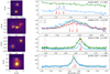 |
Fig. 1. Hα emission line maps (left) and spectra (right) of the systems observed with OSIRIS (the target name and redshift are reported in the right panels). The line maps are oriented with north being up and west to the right. The spectra shown in the right panels have been extracted over the squared apertures marked in the left panels (with the same color-coding). Each component of the systems is labeled as in Table 2. To optimize the visualization, some of the spectra have been multiplied by the factors indicated in the labels. Vertical dotted lines show the position of the main expected emission lines. |
3. Results
We find that all four targets are resolved into multiple point sources, with separations in the expected range (Mannucci et al. 2022). The images and the spectra of all the systems are shown in Fig. 1. These spatially resolved spectra allow us to study the nature of each object, as summarized in Table 2.
Summary of the results from our OSIRIS observations.
3.1. J1026+6023
J1026+6023 is composed of an AGN and a star. The AGN shows a Hα line with broad and narrow components and a prominent narrow [NII]λ6584 line with a redshift of z = 1.659. This AGN is at 0.61″ separation from the other source which has a featureless spectrum. We identify this object as most likely being a foreground star since we expect to have several of those in our sample (30% of the GMP-selected targets according to Mannucci et al. 2022), while other objects with the same spectrum are rarer. The AGN (component A) is the brightest object in the optical band, sampled by Gaia and the Sloan Digital Sky Survey (SDSS, Lyke et al. 2020), while the star is the brightest object in the near-IR H band sampled by the Keck spectra (component B).
3.2. J1608+2716
J1608+2716 is an obscured quasi-stellar object (QSO), at z = 2.575, with AV ∼ 1.8 as estimated from the SDSS spectrum. Our observations reveal three components: the central brightest one (component A), one 0.25″ to the east (component B), and one 0.29″ toward the northwest (component C). Faint extensions are visible for components A and C, but their low luminosity, compared with nearby components, and the extended wings of the AO point spread function (PSF) do not allow us to extract independent spectra. Due to the shorter wavelength range used in the observations, the spectra only cover the broad Hα line and a limited part of the continuum on both sides. All the three components show broad Hα lines at similar redshifts, with a velocity dispersion of about 5500 km s−1 full width at half maximum (FWHM), but with slightly offset line centers.
There are three main possible explanations for a triple object: (1) a triple lensed system, that is, three images of the same object; (2) lensing of a dual AGN, in other words two distinct objects, one of which has two detected lensed images; and (3) a system of three different AGNs, a possibility predicted by current models (e.g., Ni et al. 2022; Bhowmick et al. 2020; Volonteri et al. 2022) and previously observed in the local Universe (e.g., Pfeifle et al. 2019; Foord et al. 2021; Yadav et al. 2021).
To unveil the nature of this source, we can consider the following points.
Line position and profile. Component B displays both a different line profile and radial velocity with respect to the central, brightest component A, as shown in Fig. 2. Gaussian fits to the emission lines of all components show that the Hα line of component B (in blue) is centered at lower wavelengths, with a difference of ∼720 km s−1, and it has a FWHM larger than component A by 1200 km s−1. We estimated the uncertainties on the center and the FWHM of the best-fit Gaussians by adding Gaussian noise to the spectra at the observed amplitude, and computing the fit again. This process was repeated 4000 times for each line. The distribution of the resulting centers and FWHM are show in Fig. 2 (center and left panels). This shows that the differences in the center and width between components A and B are highly significant (∼7σ for FWHM and > 10σ for the center). We can exclude spatially dependent calibration issues because the sky lines in spectra extracted at the locations of the components overlap perfectly. In contrast to component B, component C has a spectrum compatible with A.
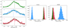 |
Fig. 2. Comparison of the Hα lines of the three components of J1608+2716. Left panels, from top to bottom: A, B, and C components, color-coded as in Fig. 1. Each panel shows the observed emission line scaled to the same flux of component A, and fit with a Gaussian profile plus a constant (shown as a thick solid line with the same color as the corresponding component). The center of the best-fitting Gaussian is reported as a vertical dashed line. For an easy comparison, the fit to component A (the brightest component) is also shown on top of components B and C. Right panels: distributions of the values of centroids and FWHM for the Gaussian fit on 4000 stochastic realizations of the observed spectra, each obtained by injecting noise into the data. |
Variability and time lag. given the small projected separation (0.25″), in the case of lensing, the time delay between components A and B is 2 days at most (Lieu 2008). For intrinsic variability to be at the origin of the differences above, this timescale must be larger than (or of the same order of) the size of the broad-line emitting region (BLR). Bentz et al. (2013) have estimated the radius of the Balmer-line emitting part of the BLR as a function of the luminosity of the continuum λL(λ) at 5100 Å. For J1608+2716, this luminosity – estimated from the SDSS spectrum and the G-band Gaia magnitude – is log(λL(λ))/erg s−1 = 46.0±0.2. For this luminosity, Bentz et al. (2013) estimate a radius of the BLR of ∼400 light-days. Even assuming that the luminosity of this object is boosted by a factor of ten by lensing, the radius would be ∼100 light-days. This is much larger than the expected delay. Therefore, in the case of lensing, no significant variability of the Hα line would be expected between the two images.
Lensing. Component C (red in Fig. 2) has a center and FWHM compatible with the brightest component, component A. However, the two lines have significantly different equivalent widths (377 Å for component A vs. 232 Å for component C). This difference, in the lensing scenario, could be attributed to microlensing of the continuum by single stars in the lensing galaxy (e.g., Hutsemékers et al. 2010). If A and C are lensed images of the same QSO, the B image would be the second component of a dual AGN, though producing a single image if it were to lie outside the radial caustic of a general elliptical mass distribution. In any case, a compact lensing galaxy should be present.
Missing lensing galaxy. Nothing is detected in the observed spectra besides the QSOs and the faint extensions of component A and C. Two lensed images of a QSO at zs = 2.57 separated by 0.25″ (with a third image strongly demagnified near the center) can be obtained with a lens galaxy with a mass of M ∼ 1010 M⊙, by assuming it at redshift zL ∼ 0.5 − 1 and by requiring the separation to be twice the Einstein radius of a singular isothermal sphere2. Such a compact lensed system would only sample the central part of the lensing galaxy where the contribution of dark matter is gravitationally subdominant with respect to stellar mass, with a contribution lower than the uncertainties. Assuming that this mass is dominated by stars, we estimate a galaxy magnitude between Ks ∼ 19.2 at z = 0.5 and Ks ∼ 20.5 at z = 1.0 (Longhetti & Saracco 2009, for an early-type galaxy with a Chabrier initial mass function). As a comparison, the QSO has Ks ∼ 19.1, estimated using Gaia magnitudes and SDSS spectra. A lensed galaxy at z = 0.5 would, therefore, be easily detected also considering that it is not a point source, while it would be below detection at z = 1, especially if it dust extincted. The nucleus of the lensing galaxy could be the faint extension of component A, which otherwise could be the QSO host galaxy.
In conclusion, the differences in line center and profile between components A and B, together with the small time delay between the images, suggest that this is not a single, triply imaged lensed QSO, but that at least two components must be present. Components A and C are compatible with a double lens system with some contribution from microlensing, with the possible detection of the host galaxy. This system would be a lensed dual QSO, similar to the system described by Lemon et al. (2022). However, since a foreground lensing galaxy is not clearly detected, this system could also be a physically triple AGN. Some knowledge of the spectral energy distribution of the three sources would further help to understand the nature of this system.
3.3. J1613+1708
J1613+1708 is a very blue QSO, with no evidence for dust extinction in the SDSS spectrum. We find that this system shows two components with similar luminosities and a separation of 0.71″ (6.1 kpc). A bright Hα line is present in both spectra, with a velocity shift of ∼500 km s−1, corresponding to redshifts of z = 1.550 and z = 1.545, respectively. The line width are also very different: 6200 km s−1 FWHM for component A, and 3100 km s−1 for component B. In the case of lensing, given its luminosity at 5100 Å of log(λL(λ)) = 45.2 ± 0.1, no significant variations of the Hα line are expected on timescales shorter than 160 days (or 50 days assuming a lensing magnification by a factor of ten, Bentz et al. 2013). In contrast, the delay expected due to the separation of the two components would be 10 days at most. As a consequence, we conclude that the two objects are associated with two different AGNs in a single host.
3.4. J2335+3201
This is a low-extinction (AV ∼ 0.4, estimated from the SDSS spectrum) system at z ∼ 0.9 showing two distinct components 0.61″ (4.8 kpc) away, with a large (∼12) luminosity ratio. We find that both objects show a broad Hα line width (FWHM = 2900 km s−1 for component A and 2700 km s−1 for component B). The two lines show a significant velocity shift of about 400 km s−1, and different line profiles. The system has log(λLλ) = 44.9 at 5100 Å, implying variability timescales of ∼100 days (30 days in the case of a lensing magnification by a factor of ten), to be compared with the expected delay of 2 days. Therefore, also in this case, the differences are better explained by a dual AGN system.
4. Conclusions
We used AO-assisted, spatially resolved spectroscopy to unveil the nature of four complex AGN systems at redshifts between 0.9 and 2.4 selected through the GMP method. As expected by the GMP selection, all of these objects show multiple components with subarcsec separations. Target J1026+6023 is best described by an AGN/star alignment (given the featureless continuum), while emission from broad lines typical of QSO are seen in all the components of the remaining three systems. Velocity shifts of a few hundred km s−1 are seen in J1608+2716, J1613+1708, and J2335+3201, compatible with being due to multiple distinct SMBHs likely to be in the process of merging inside a single host. The differences in line profiles and projected separations are indeed best reproduced by intrinsically distinct SMBHs rather than lensing by a foreground galaxy. In fact, the luminosity of the three QSOs, even allowing for possible lensing magnification, implying large sizes of the BLR and therefore slow variability on timescales of several tens or hundreds of days. Since the expected time delay between different lensed images would correspond to a few days at most, the differences cannot be due to lensing delay. Moreover, there is no evidence for a foreground lensing galaxy.
Our observations confirm that a sizeable sample of intrinsic multiple AGNs can be identified by obtaining resolved spectra of GMP-selected systems. The dual AGNs presented here are among the systems with the smallest known separations, compatible with being inside the same host galaxy. At z > 0.5, the other known systems with separations below 5 kpc were discovered either serendipitously (Junkkarinen et al. 2001; Glikman et al., in prep.) or by looking for multiple source in the Gaia archive (Chen et al. 2022), a technique that has very low efficiency at separations below 0.5″. For this reason, the number of known such systems until now had remained low despite a significant observational effort. In contrast, the GMP method provides hundreds of candidate, multiple AGNs among confirmed QSOs, and many more can be obtained by applying the GMP method to large numbers of photometrically selected QSO candidates. Future observations from the ground (especially with VLT/MUSE, VLT/ERIS, and Keck/OSIRIS) and from the space (HST/STIS, JWST/NIRSPEC) of these GMP-selected dual AGNs candidates will allow us to largely increase the number of confirmed multiple systems and begin to compare the results with theoretical predictions on galaxy formation and evolution.
The parameter of the Gaia archive used for the GMP selection.
![Mathematical equation: $ \theta_{\mathrm{E}}^{\mathrm{SIS}}=[D_{\mathrm{LS}}/(D_{\mathrm{L}} D_{\mathrm{s}})\, 4GM/c^2]^{1/2} $](/articles/aa/full_html/2023/03/aa45853-23/aa45853-23-eq1.gif) , where DL, DS are the angular diameter distances of the lens and the source, and DLS is the one between the lens and the source.
, where DL, DS are the angular diameter distances of the lens and the source, and DLS is the one between the lens and the source.
Acknowledgments
We thank the referee for constructive comments that helped improving the manuscript. AC acknowledges support from NSF AAG grant AST-1412615, Jim and Lori Keir, the W. M. Keck Observatory Keck Visiting Scholar program, the Gordon and Betty Moore Foundation, the Heising-Simons Foundation, and Howard and Astrid Preston. GC, FM, AM and EN acknowledge support by INAF Large Grants “The metal circle: a new sharp view of the baryon cycle up to Cosmic Dawn with the latest generation IFU facilities”. GC, FM, AM, EN, PS, CC and CV acknowledge support by INAF Large Grants “Dual and binary supermassive black holes in the multi-messenger era: from galaxy mergers to gravitational waves” (Bando Ricerca Fondamentale INAF 2022). GV acknowledges support from ANID program FONDECYT Postdoctorado 3200802. The authors wish to recognize and acknowledge the very significant cultural role and reverence that the summit of Maunakea has always had within the indigenous Hawaiian community. We are most fortunate to have the opportunity to conduct observations from this mountain.
References
- Begelman, M. C., Blandford, R. D., & Rees, M. J. 1980, Nature, 287, 307 [Google Scholar]
- Bentz, M. C., Denney, K. D., Grier, C. J., et al. 2013, ApJ, 767, 149 [Google Scholar]
- Bhowmick, A. K., Di Matteo, T., & Myers, A. D. 2020, MNRAS, 492, 5620 [NASA ADS] [CrossRef] [Google Scholar]
- Bolton, A. S., Treu, T., Koopmans, L. V. E., et al. 2008, ApJ, 684, 248 [NASA ADS] [CrossRef] [Google Scholar]
- Casadio, C., Blinov, D., Readhead, A. C. S., et al. 2021, MNRAS, 507, L6 [NASA ADS] [CrossRef] [Google Scholar]
- Chen, Y.-C., Hwang, H.-C., Shen, Y., et al. 2022, ApJ, 925, 162 [NASA ADS] [CrossRef] [Google Scholar]
- Colpi, M. 2014, Space Sci. Rev., 183, 189 [Google Scholar]
- Croom, S. M., Smith, R. J., Boyle, B. J., et al. 2004, MNRAS, 349, 1397 [NASA ADS] [CrossRef] [Google Scholar]
- De Rosa, A., Vignali, C., Bogdanović, T., et al. 2019, New Astron. Rev., 86, 101525 [Google Scholar]
- Feruglio, C., Ferrara, A., Bischetti, M., et al. 2017, A&A, 608, A30 [NASA ADS] [CrossRef] [EDP Sciences] [Google Scholar]
- Flesch, E. W. 2021, ArXiv e-prints [arXiv:2105.12985] [Google Scholar]
- Foord, A., Gültekin, K., Runnoe, J. C., & Koss, M. J. 2021, ApJ, 907, 71 [NASA ADS] [CrossRef] [Google Scholar]
- Hutsemékers, D., Borguet, B., Sluse, D., Riaud, P., & Anguita, T. 2010, A&A, 519, A103 [NASA ADS] [CrossRef] [EDP Sciences] [Google Scholar]
- Jin, J. J., Wu, X. B., Fu, Y., et al. 2022, ApJS, submitted [arXiv:2212.12876] [Google Scholar]
- Junkkarinen, V., Shields, G. A., Beaver, E. A., et al. 2001, ApJ, 549, L155 [CrossRef] [Google Scholar]
- Kollatschny, W., Weilbacher, P. M., Ochmann, M. W., et al. 2020, A&A, 633, A79 [EDP Sciences] [Google Scholar]
- Lackner, C. N., Silverman, J. D., Salvato, M., et al. 2014, AJ, 148, 137 [NASA ADS] [CrossRef] [Google Scholar]
- Larkin, J., Barczys, M., Krabbe, A., et al. 2006, Proc. SPIE, 6269, 62691A [NASA ADS] [CrossRef] [Google Scholar]
- Lemon, C. A., Auger, M. W., & McMahon, R. G. 2019, MNRAS, 483, 4242 [NASA ADS] [CrossRef] [Google Scholar]
- Lemon, C., Millon, M., Sluse, D., et al. 2022, A&A, 657, A113 [NASA ADS] [CrossRef] [EDP Sciences] [Google Scholar]
- Lieu, R. 2008, ApJ, 674, 75 [NASA ADS] [CrossRef] [Google Scholar]
- Lockhart, K. E., Do, T., Larkin, J. E., et al. 2019, AJ, 157, 75 [NASA ADS] [CrossRef] [Google Scholar]
- Longhetti, M., & Saracco, P. 2009, MNRAS, 394, 774 [NASA ADS] [CrossRef] [Google Scholar]
- Lyke, B. W., Higley, A. N., McLane, J. N., et al. 2020, ApJS, 250, 8 [NASA ADS] [CrossRef] [Google Scholar]
- Mannucci, F., Pancino, E., Belfiore, F., et al. 2022, Nat. Astron., 6, 1185 [NASA ADS] [CrossRef] [Google Scholar]
- Ni, Y., DiMatteo, T., Chen, N., Croft, R., & Bird, S. 2022, ApJ, 940, L49 [NASA ADS] [CrossRef] [Google Scholar]
- Pfeifle, R. W., Satyapal, S., Manzano-King, C., et al. 2019, ApJ, 883, 167 [Google Scholar]
- Planck Collaboration VI 2020, A&A, 641, A6 [NASA ADS] [CrossRef] [EDP Sciences] [Google Scholar]
- Rosas-Guevara, Y. M., Bower, R. G., McAlpine, S., Bonoli, S., & Tissera, P. B. 2019, MNRAS, 483, 2712 [NASA ADS] [CrossRef] [Google Scholar]
- Rubinur, K., Das, M., & Kharb, P. 2019, MNRAS, 484, 4933 [Google Scholar]
- Shajib, A. J., Treu, T., Birrer, S., & Sonnenfeld, A. 2021, MNRAS, 503, 2380 [Google Scholar]
- Shen, Y., Chen, Y.-C., Hwang, H.-C., et al. 2021, Nat. Astron., 5, 569 [NASA ADS] [CrossRef] [Google Scholar]
- Silverman, J. D., Tang, S., Lee, K.-G., et al. 2020, ApJ, 899, 154 [Google Scholar]
- Steinborn, L. K., Dolag, K., Comerford, J. M., et al. 2016, MNRAS, 458, 1013 [Google Scholar]
- Stemo, A., Comerford, J. M., Barrows, R. S., et al. 2021, ApJ, 923, 36 [NASA ADS] [CrossRef] [Google Scholar]
- Tang, S., Silverman, J. D., Ding, X., et al. 2021, ApJ, 922, 83 [NASA ADS] [CrossRef] [Google Scholar]
- Tozzi, G., Cresci, G., Marasco, A., et al. 2021, A&A, 648, A99 [NASA ADS] [CrossRef] [EDP Sciences] [Google Scholar]
- Tremmel, M., Karcher, M., Governato, F., et al. 2017, MNRAS, 470, 1121 [NASA ADS] [CrossRef] [Google Scholar]
- Voggel, K. T., Seth, A. C., Baumgardt, H., et al. 2022, A&A, 658, A152 [NASA ADS] [CrossRef] [EDP Sciences] [Google Scholar]
- Volonteri, M., Haardt, F., & Madau, P. 2003, ApJ, 582, 559 [Google Scholar]
- Volonteri, M., Pfister, H., Beckmann, R., et al. 2022, MNRAS, 514, 640 [NASA ADS] [CrossRef] [Google Scholar]
- Wong, K. C. 2018, in Stellar Populations and the Distance Scale, eds. J. Jensen, R. M. Rich, & R. de Grijs, ASP Conf. Ser., 514, 165 [NASA ADS] [Google Scholar]
- Yadav, J., Das, M., Barway, S., & Combes, F. 2021, A&A, 651, L9 [NASA ADS] [CrossRef] [EDP Sciences] [Google Scholar]
All Tables
Main properties of the four targets studied in this work, along with the Keck OSIRIS observational setup.
All Figures
|
Fig. 1. Hα emission line maps (left) and spectra (right) of the systems observed with OSIRIS (the target name and redshift are reported in the right panels). The line maps are oriented with north being up and west to the right. The spectra shown in the right panels have been extracted over the squared apertures marked in the left panels (with the same color-coding). Each component of the systems is labeled as in Table 2. To optimize the visualization, some of the spectra have been multiplied by the factors indicated in the labels. Vertical dotted lines show the position of the main expected emission lines. |
| In the text | |
|
Fig. 2. Comparison of the Hα lines of the three components of J1608+2716. Left panels, from top to bottom: A, B, and C components, color-coded as in Fig. 1. Each panel shows the observed emission line scaled to the same flux of component A, and fit with a Gaussian profile plus a constant (shown as a thick solid line with the same color as the corresponding component). The center of the best-fitting Gaussian is reported as a vertical dashed line. For an easy comparison, the fit to component A (the brightest component) is also shown on top of components B and C. Right panels: distributions of the values of centroids and FWHM for the Gaussian fit on 4000 stochastic realizations of the observed spectra, each obtained by injecting noise into the data. |
| In the text | |
Current usage metrics show cumulative count of Article Views (full-text article views including HTML views, PDF and ePub downloads, according to the available data) and Abstracts Views on Vision4Press platform.
Data correspond to usage on the plateform after 2015. The current usage metrics is available 48-96 hours after online publication and is updated daily on week days.
Initial download of the metrics may take a while.