| Issue |
A&A
Volume 671, March 2023
|
|
|---|---|---|
| Article Number | A31 | |
| Number of page(s) | 15 | |
| Section | Astrophysical processes | |
| DOI | https://doi.org/10.1051/0004-6361/202244687 | |
| Published online | 02 March 2023 | |
Three-dimensional solar active region magnetohydrostatic models and their stability using Euler potentials
1
Departament de Física, Universitat de les Illes Balears (UIB), 07122 Palma, Spain
2
Institute of Applied Computing & Community Code (IAC 3), UIB, 07122 Palma, Spain
e-mail: This email address is being protected from spambots. You need JavaScript enabled to view it.
3
School of Mathematics and Statistics, University of St Andrews, St Andrews KY16 9SS, UK
Received:
5
August
2022
Accepted:
3
December
2022
Abstract
Active regions (ARs) are magnetic structures typically found in the solar atmosphere. We calculated several magnetohydrostatic (MHS) equilibrium models that include the effect of a finite plasma-β and gravity and that are representative of AR structures in three dimensions. The construction of the models is based on the use of two Euler potentials, α and β, that represent the magnetic field as B = ∇α × ∇β. The ideal MHS nonlinear partial differential equations were solved numerically using finite elements in a fixed 3D rectangular domain. The boundary conditions were initially chosen to correspond to a potential magnetic field (current-free) with known analytical expressions for the corresponding Euler potentials. The distinctive feature of our model is that we incorporated the effect of shear by progressively deforming the initial potential magnetic field. This procedure is quite generic and allowed us to generate a vast variety of MHS models. The thermal structure of the ARs was incorporated through the dependence of gas pressure and temperature on the Euler potentials. Using this method, we achieved the characteristic hot and overdense plasma found in ARs, but we demonstrate that the method can also be applied to study configurations with open magnetic field lines. Furthermore, we investigated basic topologies that include neutral lines. Our focus is on the force balance of the structures, and we do not consider the energy balance in the constructed models. In addition, we addressed the difficult question of the stability of the calculated 3D models. We find that if the plasma is convectively stable, then the system is not prone, in general, to develop magnetic Rayleigh-Taylor instabilities. However, when the plasma-β is increased or the density at the core of the AR is high, then the magnetic configuration becomes unstable due to magnetic buoyancy.
Key words: Sun: magnetic fields / magnetohydrodynamics (MHD)
© The Authors 2023
 Open Access article, published by EDP Sciences, under the terms of the Creative Commons Attribution License (https://creativecommons.org/licenses/by/4.0), which permits unrestricted use, distribution, and reproduction in any medium, provided the original work is properly cited.
This article is published in open access under the Subscribe to Open model. This email address is being protected from spambots. You need JavaScript enabled to view it. to support open access publication.
1. Introduction
It is well established that the structure and dynamics of the solar corona is dominated by the magnetic field. In many structures of the corona, such as active regions (ARs) and coronal holes (CHs), magnetic forces prevail, and plasma pressure gradients and gravity are often ignored. This supposition is only valid as a first order approximation and leads to the so-called force-free field models. Even under this assumption, sophisticated numerical computations are required to calculate such force-free fields in three dimensions using the obtained magnetic field vector measured in the solar photosphere as boundary conditions (BCs; see Wiegelmann & Sakurai 2021 for a review about this topic). In other regions of the solar atmosphere, such as at the interface region between the solar photosphere and corona, the relative importance of magnetic and plasma forces change by several orders of magnitude. Zhu & Wiegelmann (2018) have focused on this problem and have solved the magnetohydrostatic (MHS) equations with the help of an optimisation principle. Other approaches have recently been applied by Zhu & Wiegelmann (2022), and a recent review of the use of 3D MHS methods for solar magnetic field extrapolation has been given by Zhu et al. (2022).
Although the assumption of zero plasma beta in the solar corona is commonly applied, it is worth assessing the possible effects of plasma pressure and gravity on the magnetic field. In particular and from the practical point of view, it is interesting to construct MHS models using methods that deviate from the current trends based on optimisation processes, relaxation techniques, or Grad-Rubin methods (see Wiegelmann & Sakurai 2021). The aim of the present paper is to use a method developed and applied in the past but that has not been extended to the 3D case, at least in the study of coronal structures. As a previous step in two dimensions, Terradas et al. (2022) have recently obtained MHS equilibrium solutions that represent CHs and ARs. Based on the works of Low (1975, 1980) and using the flux function, Terradas et al. (2022) have reproduced the main features of ARs, paying particular attention to the high pressure and diffuse background of these structures instead of the single-loop structures. The goal of this paper is to extend the previous two-dimensional work to the three-dimensional case with the purpose of having a better understanding of the effect of gas pressure and gravity on a more realistic magnetic field geometry. For reasons of simplicity, the analysis of the energetics of the system due to the presence of conduction, radiation, and heating is not considered in this work. In addition, we mostly focus on closed magnetic states representative of ARs in the solar corona.
In the present work, the extension of Terradas et al. (2022) to three dimensions is based on the use of Euler potentials (EPs) instead of the flux function. The EPs were originally devised by Euler to describe incompressible velocity fields. The application of EPs is not new in magnetohydrodynamics (MHDs), and they are most well known in the context of magnetospheric studies (see e.g. Cheng 1995; Zaharia et al. 2004; Zaharia 2008). The reader is referred to the fundamental works on the use of EPs of Stern (1967, 1970; see also Stern 1976, 1994a,b). A significant number of examples using EPs can be found in Schindler (2006) and also in studies related to magnetic reconnection (Hesse & Schindler 1988; Hesse & Birn 1993). The EPs are also referred to as Clebsch variables (e.g. Roberts 1967). Due to reasons that are discussed in more detail later in this paper, there is only a limited number of investigations that have used EPs to study magnetic structures in the solar atmosphere. Barnes & Sturrock (1972) took a model to represent the magnetic field configuration of a sunspot of one polarity surrounded by a magnetic field region of opposite polarity and used EPs to study how a force-free field structure can be metastable and converted into an open field structure by an explosive MHD instability. Zwingmann (1984, 1987) used EPs to investigate the onset mechanisms of eruptive processes in the solar corona, while Romeou & Neukirch (1999, 2001, 2002), mainly using 2D or 2.5D structures, have investigated sequences of magnetostatic equilibria that may contain bifurcation points using a similar approach as in Zwingmann (1987) and Platt & Neukirch (1994) by employing a numerical continuation method to capture the different branches of the solutions. As far as we know, the fully 3D case using EPs has not been addressed in the analysis of magnetic configurations of the solar corona, and this is one of the main purposes of the present work.
The general 3D MHS problem is quite intricate and analytical solutions are only obtained under very specific conditions (see Low 1985, 1991, 1992, 1993a,b; Neukirch 1995, 1997; Neukirch & Rastätter 1999; Neukirch & Wiegelmann 2019). The previous works are not based on EPs and essentially assume a very particular form of the current density in order to achieve analytical solutions. The use of EPs allows us a more general treatment of the problem, but the drawback is that, first, a purely numerical treatment is required in most of the cases and, second, the representation of a genuinely 3D magnetic field by two EPs exists as a global representation and is valid in the whole domain only if the magnetic field has a simple topology. In particular, we can always find EPs α and β that correctly represent the magnetic field locally, but in 3D we can only guarantee that the same EPs represent the magnetic field everywhere if the domain contains one surface in which each field line intersects only once and if the magnetic field does not have any null points (B = 0) inside the domain, or if the magnetic field has a vector potential A for which A ⋅ B = 0 (Rosner et al. 1989).
Numerical methods based on finite elements are known to be a powerful route to calculate equilibrium solutions under quite broad conditions. They have been successfully used in the past in 2D by Zwingmann et al. (1985), Zwingmann (1987), Platt & Neukirch (1994), Romeou & Neukirch (1999, 2001, 2002). This is the technique chosen in the present work to construct a wide range of MHS solutions in 3D based on EPs.
Moving to 3D is challenging for several reasons. First of all, the size of the matrices involved in the finite element discretisation increases significantly, slowing down the process of obtaining a solution. Second, an appropriate starting point or ‘seed’ of the initial distribution of the EPs in 3D is required. For this reason, we still need to use potential magnetic fields with known analytical expressions for the corresponding EPs as a starting point of our finite element calculations. Even if we know the magnetic field components, the calculation of the EPs is not straightforward. The initial states are the key ingredient for including more realistic effects, such as magnetic shear, in the configurations, and this is achieved by gradually changing the magnetic field (i.e. the EPs) on the boundaries of the domain. Therefore, a difficulty regarding the method used in this work is that it relies on the initial configuration required by the numerical method to converge and achieve a final solution. It is worth mentioning that the goal of this paper is not to use an observed magnetic field to construct an MHS solution. The main objective is to assess the benefits and difficulties of using EPs in 3D under somewhat idealised conditions.
Finally, an important question to be decided is whether the 3D equilibrium configurations that are numerically obtained are in fact stable. Due to the interplay between magnetic and buoyant forces, the magnetic Rayleigh-Taylor instability or the Parker instability may be present in the system, which is important information for assessing the relevance of the model to represent solar magnetic field configurations. The presence of electric currents can also affect the stability of the system. In the magnetospheric context, MHD eigenmodes and the calculation of field line resonances in 3D have been addressed in the past (see for example Cheng 1995, 2003; Rankin et al. 2006; Kabin et al. 2007). In this work, instead of calculating the eigenmodes of the configuration, we use the result devised by Zwingmann (1984, 1987) in the context of the study of coronal magnetic structures. Though he applied the method to 2.5D the problem of stability in 3D can still applied to the analysis of the discretised version of an operator that is needed during the calculation of the equilibrium solutions. We apply this procedure to the 3D case in the last part of this work to address the significant issue of the stability of the obtained MHS solutions.
2. Magnetohydrostatic equilibrium in three dimensions using Euler potentials
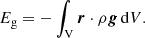
A magnetohydrostatic equilibrium must satisfy force balance; for this reason we looked for solutions to the following equation
 (1)
(1)
where B is the magnetic field, p is the gas pressure, ρ the plasma density, g the gravitational acceleration on the solar surface, and μ0 the magnetic permeability of free space. The magnetic field from Maxwell’s equations has to satisfy that
 (2)
(2)
We supposed that the plasma is composed of fully ionised hydrogen that satisfies the ideal gas law
 (3)
(3)
where T is the temperature, ℛ the gas constant, and  the mean atomic weight. The aim was to obtain solutions to the previous equations, but our system has five equations (Eqs. (1)–(3)) with six unknowns, B (three components), p, ρ, and the temperature T. An energy equation, sometimes called a heat transport equation, is required to have a closed system. For this work, we adopted the approach of Low (1975), which does not solve the energy equation directly. Once we obtained a solution, we could calculate the corresponding energy balance that the system has to satisfy in order to keep a thermal equilibrium, but this is not the main goal of the present study.
In 2D the previous MHS equations can be written in terms of the flux function, and the force balance leads to a Grad-Shafranov equation. This is the procedure adopted in Terradas et al. (2022). The functional dependence of pressure and temperature on the flux function determines how the plasma is coupled to the magnetic field. However, if we want to employ the equivalent approach in 3D, the magnetic field needs to be written in terms of two EPs α(r) and β(r), (e.g. Roberts 1967; Stern 1970, 1976). In this case we have that
 (4)
(4)
Using vector identities, it is easy to show that Eq. (2) is automatically satisfied.
The EPs are constant along the field lines of B because B ⋅ ∇α = 0 and B ⋅ ∇β = 0. Notably, this provides a method to compute α and β in the domain when B is known (see Stern 1970, and Sect. 5). This calculation is achieved, for example, by fixing the values of the EPs on the part of the boundary of positive polarity and transporting them into the domain along the lines. In this case the problem is linear.
From Eq. (4), the magnetic field components in terms of the EPs read as
 (5)
(5)
 (6)
(6)
 (7)
(7)
These equations indicate that even in the situation of a known magnetic field, the calculation of the EPs is not trivial due to the products of partial derivatives. According to Eqs. (5)–(7), each component of the magnetic field only depends on the derivatives of the EPs in the perpendicular direction to that component. Different methods to calculate the EPs are discussed in Sects. 4 and 5.
The current density is
 (8)
(8)
and the corresponding components in Cartesian coordinates contain partial derivatives of the second order at most, but each component contains up to eight different terms. The complexity of the system is significantly increased with respect to the 2D case, which is described in terms of the flux function or the vector potential.
It can be shown that in 3D the condition of force balance using the EPs reduces to the following coupled partial differential equations (see for example Birn & Schindler 1981; Schindler 2006; Neukirch 2015, and references therein)
 (9)
(9)
 (10)
(10)
 (11)
(11)
where p(α, β, z) is the gas pressure and ρ(α, β, z) is the plasma density. In the equations, we have assumed that the gravitational force is constant and pointing in the negative z-direction. Both plasma pressure and density may generally depend on the two EPs and the gravitational potential, which in our case is identical to the z-coordinate up to a constant factor. We emphasise that the partial derivatives of the pressure in Eqs. (9)–(11) are to be taken under the condition that the other variables on which the pressure depends are kept constant. In particular, the partial z-derivative in Eq. (11) is taken with the EPs being kept constant (i.e. it is a derivative taken along field lines). Using the ideal gas law, Eq. (3), the most general solution to Eq. (11) is
 (12)
(12)
where T(α, β, z) is the temperature profile that can depend on the z coordinate as well. We defined a reference pressure scale height as  , with T0 being a normalisation temperature normally taken as the coronal temperature. It is worth noting (see also Low 1975) that, in principle, p0(α, β) and T(α, β, z) could be multi-valued along the same field line. In this work we adopted the simplest case where the same functional forms of p0(α, β) and T(α, β, z) apply to all regions of space. In this situation, two points at the same height on any magnetic field line have the same pressure and temperature.
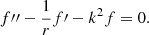
If gravity is neglected, p(α, β) = p0(α, β), meaning that pressure is constant along magnetic field lines but can change from line to line. Density was calculated from the ideal gas law using the known profiles for p(α, β, z) and T(α, β, z). Equation (12) imposes a balance between the force due to the gas pressure gradient and the gravity force along the magnetic field lines, while Eqs. (9) and (10) represent the condition of force balance perpendicular to the magnetic field. The two coupled partial differential equations (PDEs) are nonlinear, and each equation contains up to 21 different terms plus the term due to gas pressure, constituting a rather complicated system of coupled equations to solve. The equations are written in divergence form when the problem is solved numerically (see Appendix A for further details).
Equations (9) and (10) must be complemented with appropriate BCs at the limits of the domain. Here, we considered a hexahedron, in particular a rectangular cuboid. The spatial size of the cuboid is xmin ≤ x ≤ xmax, ymin ≤ y ≤ ymax, and zmin ≤ z ≤ zmax (we take zmin = 0 in this work). The BCs need to be imposed at the six sides of the cuboid to be able to solve the PDEs. A question arose as to what are the natural conditions that must be satisfied by the equilibrium equations in the variables α and β. The answer was found using Grad’s functional (Grad 1964). This author demonstrated that the first variation of the functional provides information about the nature of the BCs (see Zwingmann 1987; Schindler 2006, for a detailed derivation). There are two possibilities for the BCs. The first case corresponds to Dirichlet conditions for α and β, meaning that the EPs are prescribed on the boundaries and they are not allowed to change. Physically, this BC forces the location where a field line with labels α and β cuts through the boundary, fixing the footpoints of the field lines. For several reasons that will become clear later, we chose the potential solutions (the current-free situation) as the Dirichlet BCs. The second case corresponds to homogeneous Neumann conditions. It is not difficult to show (see Schindler 2006) that these conditions mean that the tangential component of the magnetic field on the boundaries is zero (i.e. the magnetic field is strictly normal to the boundary).
Since, in our case, we intend to reproduce the properties of a 3D AR, we preferred to focus on Dirichlet conditions and not on forcing the magnetic field to be perpendicular to the faces of the box, which seems to be rather artificial when applied to a curved magnetic field of a bipolar region. Neumann conditions are typically applied to the upper boundary when one considers the problem of magnetic configurations with different magnetic topology inside the spatial domain (see for example Zwingmann 1987; Platt & Neukirch 1994), but this is beyond of the scope of the present work.
3. General results for static ideal plasmas in equilibrium
It is appropriate to recall some known results in MHD (see for example Roberts 1967). These results are useful for interpreting some of the general properties of MHS equilibria, such as the ones we obtained from our purely numerical calculations (see also Aly 1989).
We began by introducing the gas pressure and magnetic tensors
 (13)
(13)
 (14)
(14)
where I is the unit dyadic tensor. The static equation of motion given by Eq. (1) now reads as
 (15)
(15)
If we consider a general volume V with surface S, by integrating Eq. (15) over this volume and using Gauss’s theorem, we obtain
 (16)
(16)
where dS = n dS is the directed surface element and n is the outward normal vector of the surface. The gravitational force is left as a body force, but for a self-gravitating system (different from our case), it would be more appropriate to write this force as a gravitational stress tensor similar to the gas pressure and magnetic field.
The terms that appear in Eq. (16) involve surface integrals and are inevitably related to the BCs that are imposed in the spatial domain. It is therefore relevant to clearly outline the role of the BCs in the present problem. The basic type of BCs used in this work, as mentioned earlier, are Dirichlet conditions, that is, the EPs α(x, y, z) and β(x, y, z) imposed on the side boundaries of the system. This means, according to Eqs. (5)–(7), Bn = n ⋅ B; that is, the normal component of the magnetic field is prescribed by these BCs. However, the magnetic field component lying in the plane of each boundary, Bt, depends on the behaviour in the interior points of the domain and are not fixed as they adjust according to the solution achieved inside the domain. These magnetic field components modify the inclination of the magnetic field at the boundary and change the values of the magnetic stress tensor TB.
To have equilibrium, Eq. (16) indicates that there must be a balance between forces on the surface of the volume, conditioned by the BCs, and the gravitational volume force. When gas pressure and gravity are neglected, the total magnetic stress on the surface of the volume must be zero. This does not necessarily mean that the magnetic stress is zero at all the points on the surface (in this case it is known that B = 0) but that the integrated value is zero.
Another notable general result, closely related to the conservation of energy, is the virial theorem, which is used to, among other things, check the validity of our numerical calculations in the following sections and to extract conclusions about the behaviour of the system. In the static case, the virial theorem including gravity reads as (e.g. Chandrasekhar 1961; McKee & Zweibel 1992; Kulsrud 2004)
 (17)
(17)
where r is a radius vector relative to an origin chosen to be inside the volume V and γ is typically taken to be 5/3. In the previous equation, the total internal energy is defined as
 (18)
(18)
the total magnetic energy is given by
 (19)
(19)
while the gravitational energy is
 (20)
(20)
It is important to realise that due to the Dirichlet conditions, the total magnetic energy in the system changes when, for example, gas pressure is modified, meaning that EB is not constant, even in the case when the same values of α and β are used for the different equilibria. This is due to the changes in TB, which has two contributions: one term that is fixed in this work by Dirichlet BCs and another term that changes under the presence of gas pressure and gravity in order to obtain an equilibrium.
The first two terms in Eq. (17) are always positive, but the last two terms might be negative and capable of providing the required balance in the equation. The third term corresponds to the surface pressure stress and magnetic stress, while the last term represents the integrated gravity on the volume.
4. The potential magnetic field in 3D
To find equilibrium solutions, we have shown that we need to provide the values of α and β at the boundaries (Dirichlet BCs). The EPs at the boundaries determine the global geometry of the magnetic field inside the box, and they must be chosen to represent the specific magnetic structure that is of interest, in our case the closed magnetic field lines representative of ARs. As a starting point, we used EPs that have an analytical expression, as this is typically the case for potential magnetic fields with some symmetry axis.
4.1. The magnetic bipole
One of the elementary magnetic arrangements that one can imagine in 3D relies on the superposition of fictitious monopoles that decay with distance as 1/r2,
 (21)
(21)
where a0 is a constant. We started by superposing two magnetic monopoles of opposite polarity situated below our reference plane at z = 0 at a depth z = −z0 and separated at a distance d from the origin. The magnetic field components of this structure in Cartesian coordinates are
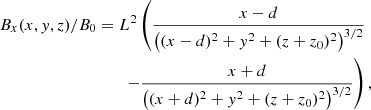 (22)
(22)
 (23)
(23)
 (24)
(24)
where L is a distance used for normalisation purposes that is equal to the pressure scale height H previously defined. This magnetic field is current-free and three-dimensional, but it still has axial symmetry. This configuration has been used in the past by, for example, Semel (1988) and Cuperman et al. (1989).
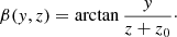
The next step was to describe the previous magnetic field in terms of the EPs, given by Eqs. (5)–(7). As explained in Sect. 2, these equations are nonlinear and generally difficult to solve for α and β, even if Bx, By, and Bz are known functions, as in the present case. However, the symmetry of the magnetic bipole (rotational symmetry with respect to the line that connects the two monopoles) allowed us to derive the corresponding EPs. As a geometrically simpler example, we first considered an arcade that is invariant in the y-direction (e.g. the arrangement investigated by Zwingmann 1987). In the case without shear, the second EP is β = y, while α is just the flux function (or vice versa). Isocontours of β are vertical planes that are labelled according to the value of y. When applying this geometrical property to the rotationally symmetrical bipole, we simply have that β = θ, with θ being the angle with respect to the line that connects the two monopoles. Therefore, in Cartesian coordinates we have that
 (25)
(25)
Since ∂xβ = 0, it was easy to calculate the EP α by direct integration of Eqs. (5)–(7),
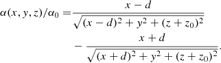 (26)
(26)
An example of the spatial distribution of α and β in 3D based on the previous expressions is shown in Fig. 1. The intersection of different isosurfaces of constant α and β coincide with the magnetic field lines. Hence, each magnetic field line is characterised by a pair of values (α, β).
 |
Fig. 1. Sketch of the bipolar configuration. Potential magnetic field lines (pink curves with arrows) and two magnetic surfaces associated to the EPs α (green color) and β (brown color) for a bipole with d = 0.25 and z0 = 0.5 (all the lengths are hereafter normalised to H). The intersection of the two surfaces, see the yellow curve, represents a particular magnetic field line. The distribution of the vertical component of the magnetic field at z = 0 is represented in gray colors. |
It is not difficult to check that the EPs given by Eqs. (25) and (26) satisfy, according to Eq. (8), that Jx = Jy = Jz = 0. This means that the magnetic field is potential and Eqs. (9) and (10) are fulfilled since the gas pressure has no effect on the equilibrium configuration in this case.
Since the potential solution has rotational symmetry, it is appropriate to use cylindrical coordinates instead of Cartesian coordinates. The solution given by Eqs. (25) and (26) in cylindrical coordinates reads as
 (27)
(27)
as indicated earlier, while
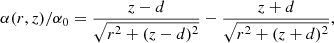 (28)
(28)
being independent of θ. The z-coordinate now points along the symmetry axis in this new coordinate system (the x-direction in the Cartesian coordinates).
The EPs are not unique since a different gauge leads to the same magnetic field, but it is beneficial to choose the most simple geometrical surfaces for the EPs. For example, we have shown that the symmetric bipolar magnetic field β can be represented by planes, and this is our preferred option, see Fig. 1.
4.2. The general analytic solution for the case with axial symmetry
In the case where the pressure gradient either vanishes or is in hydrostatic equilibrium with the gravitational force, the potential structure in cylindrical coordinates is a solution to the following equations (see also Kaiser & Salat 1997)
 (29)
(29)
![Mathematical equation: $$ \begin{aligned}&\partial _\theta \left(\frac{1}{2\mu _0}\frac{1}{r^2}\left[(\partial _r \alpha )^2+(\partial _z \alpha )^2\right]\right)=0. \end{aligned} $$](/articles/aa/full_html/2023/03/aa44687-22/aa44687-22-eq32.gif) (30)
(30)
Assuming that α is independent of θ, the second equation was automatically satisfied, and we only had to solve the first equation. The simple bipole model given by Eq. (28) satisfies this equation. However, it is useful to generalise the method of finding the potential solution for any magnetic spatial distribution on the axis, α(0, z), and this is the purpose of the present section. As far as we know, the following derivation has not been reported in the literature.
In order to avoid undesirable boundary effects, we wished to solve Eq. (29) by imposing that α = 0 for r → ∞. We used the method of separation of variables and assumed that
 (31)
(31)
which led to
 (32)
(32)
with k being the separation parameter and the derivatives being related to the arguments of the functions. We obtained two separate ordinary differential equations (ODEs) that share the parameter k. The easiest ODE to solve corresponds to the z-dependence and reads as
 (33)
(33)
The solution to this equation is a superposition of a sine and a cosine function,
 (34)
(34)
with A and B as constants that need to be determined. The separation parameter k appears in the argument of the functions.
Returning to Eq. (32), the ODE for the radial part is
 (35)
(35)
To solve this equation, we assumed that f(r) = rℱ(kr) which is inserted into Eq. (35). This process led to a modified Bessel equation for ℱ(kr), meaning that the general solution to Eq. (35) is of the form
![Mathematical equation: $$ \begin{aligned} f(r)=r\left[C\, I_1(kr)+D\, K_1 (kr)\right], \end{aligned} $$](/articles/aa/full_html/2023/03/aa44687-22/aa44687-22-eq38.gif) (36)
(36)
where I1(kr) and K1(kr) are the modified Bessel functions of order one, while C and D are constants that need to be determined according to the BCs.
For r → ∞ we had that rI1(kr)→∞, and therefore, we had to impose C = 0 to avoid this behaviour. In contrast,  for large r, which means that this solution goes to zero at infinity. For r → 0, rK1(kr)≃1/k and has the correct behaviour at the origin (finite and different from zero in general).
The formal solution to our problem, taking into account the z and r dependencies, is the following superposition
![Mathematical equation: $$ \begin{aligned} \alpha (r,z)=\int _0^\infty \left[A(k) \cos (k z)+B(k) \sin (k z)\right]\, r\, K_1(k r) \, \mathrm{d}k. \end{aligned} $$](/articles/aa/full_html/2023/03/aa44687-22/aa44687-22-eq40.gif) (37)
(37)
The Fourier coefficients A(k) and B(k) were determined from the chosen profile for α at r = 0 (i.e. on the axis), which according to the previous expression is
![Mathematical equation: $$ \begin{aligned} \alpha (0,z) = \int _0^\infty \left[A(k) \cos (k z)+B(k) \sin (k z)\right]\frac{1}{k} \, \mathrm{d}k, \end{aligned} $$](/articles/aa/full_html/2023/03/aa44687-22/aa44687-22-eq41.gif) (38)
(38)
where the value at the origin of rK1(kr) has been taken into account. Using the known result from Fourier analysis, the coefficients read as
 (39)
(39)
 (40)
(40)
If α(0, z) is a symmetric function with respect to z = 0, then B(k) = 0, whereas if it is anti-symmetric, A(k) = 0.
The main result of this section is that we found a general expression, Eq. (37), that allows us to calculate the potential solution in the r − z plane given any profile of α on the axis (i.e. α(0, z)). This solution is used later as a BC to construct MHS equilibria in 3D under the presence of gas pressure and gravity. It is also adopted as the starting point to include magnetic shear in the structure. A simple test of the validity of the previous expressions was achieved by reproducing the double monopole potential solution given by Eq. (28).
A similar approach can be applied to the case with the effect of the gas pressure included, as long as the derivative of this magnitude with α is proportional to α, that is, the linear case (see the analysis performed in Atanasiu et al. 2004). When gravity is also present, no analytic solutions are available, as far as we know.
The relevance of the procedure used to construct a solution became clear when we considered an example of a structure that lacks symmetry along the axis, that is, a structure that is not symmetric around z = 0 (in cylindrical coordinates). The first step of the procedure was to choose the particular form of α(0, z). In order to simplify the calculations, we chose a profile that leads to analytical results for the Fourier coefficients. Our deliberate choice is a Gaussian function
 (41)
(41)
situated at zs (not necessarily equal to zero) and with a characteristic width w and C as a constant. Substituting this expression into Eqs. (39) and (40) and performing the integrals (see Gradshteyn & Ryzhik 2007) yielded
 (42)
(42)
 (43)
(43)
The solution α(r, z) was obtained by substituting the previous coefficients in Eq. (37) and integrating with respect to k. This integral over the semi-infinite range does not have an analytical solution and must be calculated numerically. We used MATHEMATICA to compute the integral.
Since Eq. (29) is a linear PDE, a superposition of, for example, several Gaussian profiles at distinct locations and with different amplitudes can be readily constructed using the previous expressions. Once the profile α(r, z) was known, a change from cylindrical to Cartesian coordinates was needed, and taking into account that our reference level is located at zmin, the symmetry axis in cylindrical coordinates was situated at a depth zd below zmin. In Fig. 2, we show an example of the superposition of two Gaussian profiles with certain values as the parameters. In this case, the two constants, C1 and C2, have opposite signs. The constructed structure has a central region where the magnetic field is open, as can be seen on the top face of the box in Fig. 2, and can represent a CH that is surrounded by two ARs with closed field lines. The configuration still has rotational symmetry because surfaces of constant β are still planes.
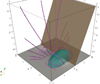 |
Fig. 2. Potential magnetic field lines and isosurfaces calculated numerically for a non-symmetric case along x-direction. In this example, the following parameters have been used: w1 = w2 = 1/4, z1 = −3/4, z2 = 1, C1 = 1, and C2 = −0.5. |
Interestingly, if we assume that the factors C1 and C2 have the same sign, which is the opposite of the situation shown in Fig. 2, the topology of the magnetic field changes, and it may happen that at some points the magnetic field becomes zero, i.e., there are magnetic null points. According to the definition of the magnetic field in terms of the EPs and due to the symmetry in the azimuthal direction assumed in this section (β = θ), the only possibility to satisfy B = 0 is that ∇α = 0. Since α depends on r and z only, the last condition means that at a magnetic null point, which is precisely a critical point in a mathematical sense, α(r, z) has either a local minimum, a local maximum, or a saddle point. Minima or maxima of α correspond to O-type magnetic nulls, whereas saddle points correspond to X-type null points. An example that includes an X-type magnetic field structure is shown in Fig. 3. In reality, this is actually a null line (a curve where the magnetic field vanishes) due to the rotational symmetry. Therefore, this structure is essentially an X-point in a 2D sense since the characteristics of a truly 3D null point are not present and there is no spine line or fan plane (see for example Parnell et al. 1996; Priest & Forbes 2007). The connectivity of the magnetic field lines changes when moving across the separatrix surfaces that intersect at the null line. It is known that, contrary to isolated 3D null points, null lines can be locally described using EPs (see Hesse & Schindler 1988), as in the present case. However, it is also known that magnetic null lines are structurally unstable, and any arbitrarily small additional magnetic field will either generate a magnetic field without nulls or one with isolated nulls (e.g. Schindler et al. 1988).
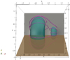 |
Fig. 3. Potential magnetic field lines and isosurfaces that include X-points. A visible critical point is located around x = 0.5 and y = 0.5, but due to rotational symmetry, it is repeated along a circular path, and in reality, it is a null line. The same parameters as in Fig. 2 were used except that C1 and C2 have the same sign in this case. |
5. The non-potential magnetic field in 3D: Incorporating the effect of shear
The general potential solutions presented in the previous section have rotational symmetry with respect to the axis underneath zmin, where we prescribed the form of α. These solutions do not explicitly include shear and hence no field-aligned component of the current density is included either. In this section, we discuss different methods for incorporating magnetic shear into the magnetic structure in order to yield non-potential solutions. The problem is not straightforward since we needed to work with the EPs instead of the magnetic field components, but there are several possible approaches to attack this problem.
The first method is based on the use of known analytical expressions for sheared bipolar magnetic configurations. For example, Cuperman et al. (1989) gave the three magnetic field components in terms of a parameter that measures the amount of shear in the structure. This parameter is called here a (a = 0 corresponds to the potential solution given by Eqs. (22)–(24)). Even with the known expressions for the magnetic field components, the calculation of the corresponding EPs when a is different from zero is not an easy task due to the nonlinear character of the equations. One possible way to perform the calculation is to use an asymptotic expansion, as in, for example, Birn & Schindler (1981; see the explanation for the technique in Schindler 2006), to obtain approximate expressions for the EPs. This approach turned out to be rather involved, and we could not find analytical or semi-analytical solutions. Another option is to calculate α and β numerically using the computation of the magnetic field lines, which are known in this case, as was proposed by Stern (1970). The idea is that if the EPs are known on a given surface, then tracking the intersection of any field line with this surface will provide the values of the EPs on the magnetic field lines and therefore of any point of the domain (as long as all the field lines intersect the reference surface). The foremost limitation of this method is that the magnetic field distribution in 3D must be known in order to calculate the EPs, and this is not the typical situation.
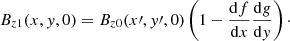
We propose here a method that we think is more flexible than the previous approaches. It is based on transforming the Euler variables in the potential situation in such a way that they lead to magnetically sheared states. Again, gas pressure and gravity are added once the magnetic force-free solution is obtained. The method is based on directly shearing the EPs at z = 0 as well as at the other faces of the box while still keeping a rectangular shape for the domain. To do so, we applied an affine coordinate shear transformation defined by x′=x + syy and y′=sxx + y, where sx and sy are the shear factors in the x- and y-directions. This transformation produced the effect on the magnetic field we sought, as demonstrated in the following equations. For example, the vertical component of the magnetic field at z = 0 is, according to Eq. (7),
 (44)
(44)
and the shear transformation changes Bz0 to Bz1
 (45)
(45)
Using the chain rule for multi-variable functions and the coordinate transformation, it is not difficult to find that the previous expression reduces to
 (46)
(46)
meaning that the final magnetic field is the initial magnetic profile but sheared, due to the presence of the primed coordinates in the argument of Bz0, times a factor that is proportional to the shear parameters in each direction. The same applied to the magnetic field components perpendicular to the rest of the faces of the box.
The previous idea of applying a deformation to the EPs was developed further, and we defined another transformation
 (47)
(47)
 (48)
(48)
which can be shown as leading to
 (49)
(49)
At this point, the functions f(x) and g(y) could be appropriately chosen to make the parenthesis of the previous equation independent of x and y, ensuring that the transformation of the EPs produced exactly the expected shear on the vertical component of the magnetic field. The shear transformation previously discussed fits into this category as a particular case (where f(x) = sxx and g(y) = syy), but there are alternative approaches that can allow for the incorporation of families of changes on the magnetic field that are not necessarily affine transformations. For example, one approach starts with a potential solution that is axially symmetric, and through a transformation, it achieves a non-symmetric solution. For example, we chose
 (50)
(50)
 (51)
(51)
This transformation makes the parenthesis of Eq. (49) equal to one and produces the effect of shifting the magnetic field around x = x0 in the y-direction an amount a0 within a typical distance w. This is a rather simple way of creating non-symmetric profiles for the EPs when starting from known symmetric solutions. Examples of the two transformations applied to the EPs explained in this section and that led to particular sheared magnetic field configurations are discussed in Sect. 7.3.
6. The numerical method
Once we had an initial magnetic distribution uncoupled from the plasma, our goal was to find solutions to Eqs. (9) and (10). Unfortunately, analytical solutions to these equations are extraordinarily difficult to obtain, especially if the effect of gas pressure and gravity are included in the model. Ignoring gravity and gas pressure may lead to analytical solutions under some symmetry conditions, and some examples are shown in Sect. 4.2. But, in general, numerical techniques are required to obtain solutions to the equilibrium equations. In the present work, in order to solve the PDEs with the corresponding BCs, we used the finite element method (for details see, e.g. Zienkiewicz et al. 2013; Ganesan & Tobiska 2017).
We used the finite element method implemented in MATHEMATICA to solve linear and nonlinear PDEs. In general, we found the software to have a good performance when using parallelisation to speed up the computation time. The PDEs, according to the requirements of MATHEMATICA, must be introduced into the code in divergence form (see Appendix A). In addition to the BCs at the six faces of the cuboid, an initial condition for the solution is required by the numerical algorithm. We chose the potential solution that was calculated using the analytical expressions of Sect. 4 and applied the procedure to include shear, explained in Sect. 5, as the initial condition. The problems addressed in the present work do not require the use of continuation methods to calculate sequences of equilibria and detect the presence of bifurcation points (see for example Neukirch 1993a,b; Romeou & Neukirch 1999). The simple strategy of slowly varying a parameter, calculating a solution, and using it as the initial condition for the following step has been shown to be sufficient for the type of equilibria considered in this paper.
In most of the calculations, we used a non-uniform numerical mesh with refinement around the region where the strongest magnetic field is prescribed, i.e., around the center of the face z = zmin. An example of the mesh is shown in Fig. 4. In this configuration the mesh is basically the product of three non-uniform meshes, two of them refined around the center (in the x- and y-directions) and another refined around zmin.
 |
Fig. 4. Typical mesh structure used in finite element calculations. The x-axis and y-axis point along the orange and green faces of the box, while the z-axis is vertical. A non-uniform grid in each direction has been used to improve the accuracy of the calculations. The most refined region of the grid is located around x = y = z = 0. In this example, the grid has 62 500 elements. |
Several tests were performed to validate the obtained numerical solutions. The first test considered the potential case (no gas pressure or gravity) and used the analytical potential solution given by Eqs. (25) and (26) as BCs at the six faces of the cuboid and also as the initial condition for the whole 3D box. The discrepancies between the numerically computed solution and the analytical results are very small and decrease as the number of mesh elements is increased. For non-potential calculations, using the potential solution again as the BC and as the initial condition, we calculated the corresponding volumetric and surface integrals in Eq. (17) for the numerically obtained solutions. The computations indicated that the numerical error in the expression of the virial theorem is typically around 2% and becomes smaller when the number of finite elements is increased. This is a clear indication that the calculated equilibria under the presence of gas pressure and gravity are correct.
The numerical difficulties found in the present problem are in some cases related to the fact that the initial condition is not sufficiently close to the actual solution. Another difficulty is due to the potential solution being imposed at the boundaries, especially at the upper boundary, which may lead to convergence issues because the system is forced to satisfy the BCs even under the presence of other forces, such as the gas pressure gradient and the gravity force. This last issue is more relevant in the case where the plasma-β exceeds the value of one near the upper boundary.
7. Equilibrium calculations: Numerical results
The inclusion of gas pressure and gravity changes the behaviour of the magnetic field and leads to a non-potential structure that needs to be computed. The functional dependencies of gas pressure and temperature on the EPs allowed us to calculate a wide range equilibrium configurations. We began with the most simple cases and proceeded with gradually more complex models.
We assume that temperature does not depend explicitly on the coordinate z (which is not a constraint in the equations considered here). In this case, Eq. (12) leads to the exponentially stratified atmosphere of the form
 (52)
(52)
The isothermal assumption along the magnetic field lines has some implications regarding the stability of the system and is discussed in Sect. 8. In the next section, we concentrate on the analysis of different equilibrium configurations.
7.1. Functional dependence on α
In obtaining an equilibrium, we have the freedom to prescribe the functional dependence of pressure and temperature on α and β. For simplicity, we focused on the situation that is independent of β. A useful functional dependence for gas pressure is
 (53)
(53)
where pC is the coronal pressure, pAR the AR pressure, and αref a reference value used for normalisation purposes. We assumed that pAR > pC, and since the dependence in Eq. (53) is upon the square of α, we ensured that gas pressure was positive everywhere (α is not necessarily a positive number). A possible choice for the temperature is,
 (54)
(54)
where TC is the coronal pressure and TAR the temperature at the core of the AR (we assumed that TAR > TC). When applying the ideal gas law at the center of the structure and at the reference coronal part, it is not difficult to find the following relationship:
 (55)
(55)
The condition pAR/pC > TAR/TC needs to be satisfied in order to represent an overdense region with respect to the environment. In this paper, we typically impose that TAR/TC = 2, i.e., the AR core is assumed to be twice as warm as the coronal environment, and pAR/pC is taken to be at least four, although larger values are used in some special cases. We note that the plasma density was calculated from the ideal gas law using the pressure and temperature profiles that are known once α(x, y, z) and β(x, y, z) have been obtained numerically.
7.2. Elementary example
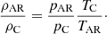
An example of an equilibrium numerically obtained with the previous pressure and temperature dependencies on α is shown in Fig. 5. The figure shows not only the bipolar distribution of the magnetic field but also the density concentration at the core of the AR. As the modified plasma-β increases, the bipolar magnetic field expands to compensate for the effect of a high pressure core. This effect is evident when comparing the top panel and bottom panel of Fig. 5. The magnetic field lines that show the largest displacements are located at the lobes of the bipolar region. This feature can be explained by the interplay of the different forces. We concentrate on the line that starts at x = 0, y = 0, z = 0 and ends at x = 0, y = 0, z = zmax. This line matches with the apex of all the magnetic field lines that are on the plane y = 0. In the potential case, at any point on the line there is a balance between the tension force pointing downward and the magnetic pressure force pointing upward. In the non-potential situation, a new equilibrium is achieved on our reference line where the magnetic tension and the gravity force point downward while the total pressure force (gas plus magnetic) points upward, balancing out the total downward force. In comparison to the potential case, the magnetic forces are weaker, and the magnetic field lines are displaced in the vertical direction. This last effect is more visible at the sides of the bipolar region where the gravity force is not aligned with the tension force as it is in our central reference line. In fact, these magnetic field lines are not coplanar, although this feature is not visible in the plots.
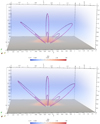 |
Fig. 5. Three dimensional bipolar configuration. Magnetic field lines and volume density (normalised to coronal density) for β00 = 1.4 × 10⁻³ (top panel) and for β00 = 1.4 × 10⁻¹ (bottom panel). In this example pAR = 4 pC, TAR = 2 TC, d = 0.25, z0 = 0.1 and αref = α(0, 0, 0). |
From Fig. 5 we also realised that the density enhancement across the core of the AR in the x-direction has a shorter spatial scale than that along the y-direction, where the density is much more elongated. This is because α changes more rapidly in the x than in the y coordinate and this affects the pressure, the temperature, and thus the density distribution of the AR. The rotational symmetry of the magnetic field also contributes to the presence of elongated structures in the y-direction.
The temperature distribution of the AR is displayed in Fig. 6. It shows a hot core at 2 MK that smoothly matches with the coronal temperature of 1 MK of the environment. The spatial distribution of the temperature and the density within the core of the AR are not exactly identical (compare Fig. 6 with Fig. 5). In particular, the temperature is more localised towards the center of the AR. We note that the density was constructed from the ideal gas law using the assumed profiles for pressure and temperature, which depend only on α.
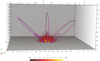 |
Fig. 6. Magnetic field lines and temperature volume for same model as in Fig. 5, bottom panel. Temperature is normalised to 1 MK. |
The local plasma-β is another quantity of relevance for the equilibrium. It is shown in Fig. 7 as a set of concentric isosurfaces. At the AR core, this parameter is rather low, typically below 0.001, but moving outwards, the values continuously increase. The plasma-β in the system can be well above one depending on the value of β00. This value agrees with the inferred behaviour from observations. Gary (2001) found that although the plasma-β is typically below one in the corona, it takes values greater than one below the chromosphere (not included in our model), and when moving from the photosphere upwards, it can return to values around 1 at relatively low coronal heights, typically of the order of 1.2 solar radii. Therefore, values of the plasma-β larger than one near the upper boundary of our domain should not be considered as unrealistic.
 |
Fig. 7. Magnetic field lines and plasma-β isosurfaces. The three isosurfaces represent values of 0.1, 0.01, and 0.001 when moving from the exterior to the interior surfaces. This example corresponds to the case shown in Fig. 5, top panel. |
To understand the effect of changing the plasma-β in the system, we varied this parameter and calculated a set of equilibria using the symmetric bipole as a BC. For each equilibrium, we computed the different terms in the virial theorem, Eq. (17), by numerically evaluating the surface integrals in 2D and the volumetric integrals in 3D. As mentioned earlier in Sect. 6, the agreement of the numerical results with the virial theorem is excellent, which is an indication of the quality of the numerical solutions.
7.3. Compound examples
Once we knew the main characteristics of the simple symmetric bipolar magnetic field, we explored other setups. We used the results presented in Sect. 5 to construct a variety of models that might be of interest and that were used as BCs. We began by including magnetic shear, and as in the previous sections, we started with the initial reference potential solution and then continued by gradually increasing the parameters sx and sy related to the affine shear transformation.
An example of a three-dimensional sheared solution is shown in Fig. 8. In the figure, the deformations of the isosurfaces of the two EPs are evident and are shown to be produced by the magnetic shear that can be seen at z = 0 in the vertical distribution of the magnetic field. The symmetry is lost in comparison to the potential case, compare with Fig. 1. A method to quantify the amount of shear in the configuration is to compute the integrated current helicity, defined as HC = ∫VB ⋅ J dV. For a purely potential magnetic field, we have that HC = 0 (since J = 0). The current helicity is different from zero when the magnetic field is force-free (J × B = 0, but J ≠ 0). We basically found a linear increase of HC with sy. The inclusion of gas pressure and gravity modified the magnetic structure of the AR as well. There is a dense and hot plasma core in the present example (similar to that in Fig. 5 but not symmetric; this is not shown in Fig. 8). We highlight that the intersection of the EP β with the computational box is always a straight line, which is due to the applied BCs. But as a consequence of the applied shear, the constant β planes are instead inclined with respect to the sides of the box in the y-direction (compare, for example, with Fig. 1).
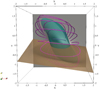 |
Fig. 8. Non-potential magnetic field lines and magnetic isosurfaces calculated numerically by applying an affine shear transformation on the EPs with sy = 0.6 and sx = sy/4. Gas pressure and gravity are included. In this model, the minimum plasma beta is around 1.4 × 10⁻³, while the maximum is around 2.5, which is well above one. In this example, we used a bipole with d = 0.25 and z0 = 0.5 in the domain xmin = −2, xmax = 2, ymin = −2, ymax = 2, zmin = 0, and zmax = 4. |
Next, we applied the transformation to the EPs using the displacement of the polarities on the plane z = 0 given by Eq. (51). The obtained non-symmetric structure is shown in Fig. 9. The example in this figure indicates the presence of regions with open magnetic fields close to one of the footpoints of the AR, and it represents the extension of the case shown in Fig. 2. This equilibrium could be used to model the interaction of an AR and a CH, as was done in 2D in Terradas et al. (2022). The intersection of the EP β with the upper and lower boundaries of the computational box is not a straight line and is produced by the specific transformation used in this example. Interestingly, although not displayed in Fig. 9, the density is high within the core of the ARs but low (below the coronal reference value) where the magnetic field lines are open. This behaviour is due to the dependence of gas pressure and temperature on α and agrees with the expected behaviour in CHs.
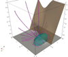 |
Fig. 9. Non-potential magnetic field lines and isosurfaces calculated numerically by applying transformation on EPs using Eq. (51). Gas pressure and gravity are present. Compare with Fig. 2. In this configuration, a0 = 0.6, x0 = 1, w = 1, β00 = 1.4 × 10⁻³, and αref = α(−1, 0, 0). |
Finally, the density profile for a situation that contains a magnetic null line is shown in Fig. 10, and it is based on the example shown in Fig. 3. We have included a small amount of magnetic shear using the transformation applied in the previous example. We found a rather non-uniform distribution of the density, but most of the mass is located in the bipolar region around x = −1, which is where the plasma has the maximum temperatures because, according to our model, α2 has a maximum there. Around the null line, the density and temperature are rather low. The numerical method is able to converge to an equilibrium solution that contains both an ordinary AR and a nearby null line under the presence of gas pressure and gravity.
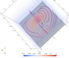 |
Fig. 10. Magnetic field lines and volume density (normalised to the coronal density) for a situation that contains a null line. In this example, magnetic shear with a0 = 0.3, x0 = 1, and w = 1 has been induced in the structure. Gas pressure and gravity are present with β00 = 1.4 × 10⁻³. |
According to the different examples shown in this section, we can affirm that the EPs are useful for calculating a variety of, not necessarily simple, magnetic structures in which the plasma is coupled to the magnetic field. These configurations can be used to represent ARs in the solar atmosphere either as isolated entities or as companions of open magnetic field regions or even to describe more involved magnetic topologies that contain null lines.
8. Stability analysis of the calculated equilibria
So far we have concentrated on the calculation and analysis of equilibria in 3D, but their stability has not been addressed yet. A question that arose was whether the interplay between the magnetic field, gas pressure, and gravity may lead to the appearance of magnetic Rayleigh-Taylor instabilities or Parker instabilities. There are two modes of the magnetic buoyancy instability: the undular mode with a wavenumber parallel to the magnetic field and the interchange mode with a wavenumber perpendicular to B. The undular mode is often called the Parker instability, after Parker (1966). The interchange mode is often referred to as the flute instability or the magnetic Rayleigh-Taylor instability. The undular mode occurs for long wavelength perturbations along the magnetic field lines, and the plasma tends to slide downward along the field from the peaks into the valleys, further enhancing the undulations. In contrast, the interchange mode occurs for short wavelength perturbations, when the interchange of two straight flux tubes reduces the potential energy in the system. Nevertheless, the most unstable mode has a 3D structure and therefore has both a wavevector component parallel and perpendicular to the magnetic field. The instability typically occurs for short wavelengths in the transverse direction, but it is highly dependent on the wavelength parallel along the field. This instability is completely suppressed for short parallel wavelengths (see for example, Fig. 13.1 in Parker 1979).
In general, an equilibrium is stable if and only if the change in the potential energy, δW, associated to all allowable displacements satisfying appropriate BCs is always positive, that is, δW ≥ 0. When the equilibrium configuration is complex (three-dimensional curved magnetic field in balance with the pressure gradient and the gravity force), the estimation of the sign of the potential energy must inevitably be computed by numerical means. Here we give further details about a numerical approach that has received little attention in the literature but that is of considerable utility. Zwingmann (1984, 1987; see also Schindler 2006) generalised the stability criteria found by Schindler et al. (1983) and Hood (1984) to three dimensions and showed that the potential energy can be split into two parts
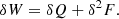 (56)
(56)
The term δQ accounts for the purely convective instability, and a stable situation is achieved when (see for example Schindler et al. 1983)
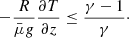 (57)
(57)
This condition is the Schwarzschild criterion for stability against convection modes projected along the magnetic field lines. In our case, according to Eq. (52), there is no explicit dependence of temperature upon z (but we note that α and β depend on x, y, and also z). Therefore, the previous condition is always satisfied, and the system is convectively stable.
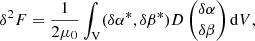
The second term in Eq. (56) can be written as
 (58)
(58)
where D is a linear operator written as a 2 × 2 matrix, where we have defined δα = −ξ ⋅ ∇α, δβ = −ξ ⋅ ∇β, and where ξ represents the displacement vector. We constructed the matrix M, which is the numerical equivalent of the linear MHD operator D when we performed a discretisation, using finite elements. From the mathematical point of view, the matrix M is positive definite if xTMx > 0 for any vector x (as xT is its transpose), and this is in essence the integrand in Eq. (58). Therefore, if M is positive definite, then the equilibrium is stable and any changes of M from positive definite to non-definite indicate a transition from stable to unstable solutions. This change is due to the fact that this matrix is the numerically discretised equivalent of a sufficient stability functional (when purely convective instabilities are not present in the system), and it turns out that δ2F is the second variation of the free-energy functional introduced by Grad (1964). This method based on the analysis of the matrix M has been successfully used in 2D studies (e.g. Zwingmann 1987; Platt & Neukirch 1994; Neukirch & Romeou 2010). If the configuration is three-dimensional, this approach is still valid but involves significantly larger matrices than in the 2D case and therefore more computationally intensive calculations. The disadvantage of the method is that it does not provide the frequency or the growth rates of the unstable modes. It just classifies the system as stable or unstable, which is nevertheless a valuable piece of information.
With the procedure now clear, after obtaining a solution to the equilibrium equations, the matrix M associated to the linear operator was constructed, and its positiveness was evaluated to assess the stability of the solution. MATHEMATICA has implemented a command to test if a matrix is positive definite. In the work of Zwingmann (1987), the linearised operator is also needed to solve the equilibrium equations, but in our case, it is better to construct the matrix M a posteriori once the equilibrium has been computed. Details about the linear operator are given in Appendix B.
8.1. Parker’s instability test: Horizontal magnetic field
As a test of the numerical procedure based on the matrix M, we considered the simplified case of a purely horizontal magnetic field coupled to gas pressure. Pressure, density, and magnetic field decay exponentially with height, but the sound and Alfvén speeds are constant, allowing a normal model analysis. The details about the stability analysis of this elementary configuration can be found in Parker (1966, 1979). The general dispersion relation is given by Eq. (13.33) of Parker (1979) and depends on the choice of the wavenumbers in the three directions, kx, ky, and kz, as well as the value of the plasma-β (constant in the domain). The frequency switches from purely real to purely imaginary, meaning that the system changes from stable to an unstable state.
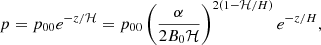
We derived the EPs associated to the previous equilibrium with the magnetic field pointing in the x-direction, which read as
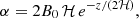 (59)
(59)
 (60)
(60)
while gas pressure is
 (61)
(61)
and has been written in terms of the EP α. Here, ℋ = H + H/β00 is the modified pressure scale height that couples the plasma to the magnetic field (H is the isothermal scale height). The key parameters of this problem are β00 and the wavelengths that fit in our computational box, namely,
 (62)
(62)
 (63)
(63)
 (64)
(64)
Using the previous expressions, we tested the stability of the system with the positive definiteness of the matrix M constructed using finite elements. We found that the positive definiteness of M changes precisely when the dispersion relation given by Parker predicts a transformation of a stable solution into an unstable solution and vice versa. This match indicates that the numerical method was correctly implemented and can be confidently used to investigate the stability of more complex equilibria. Small deviations from the theoretical predictions are related to the fact that in our calculations, we are imposing strict line-tying conditions, while in Parker’s calculations, Fourier analysis without imposing line-tying was performed.
8.2. Results for the computed 3D equilibria
When the reference plasma-β is very small, most of the numerically calculated equilibria described in Sect. 7 are found to be stable. However, we have found that increasing this parameter and changing the pressure contrast (density contrast between the AR and the environment) may lead to unstable structures. An example of a stability diagram based on the bipole considered in Sect. 4.1 is shown in Fig. 11. For a fixed reference plasma-β, β00, we always found that by increasing the density contrast at the core of the AR, the configuration becomes unstable at some point, meaning that a small perturbation in the system will automatically lead to the growth of the perturbation. The magnetic field cannot support, under stable conditions, the extra mass load due to the increase of the density contrast. When the plasma-β is very small and therefore the magnetic field is very strong in comparison to the gas pressure, increasing the amount of mass at the core of the AR makes the model unstable only for very large and unrealistic density contrasts according to Fig. 11. This behaviour is as it would be expected from the physical point of view.
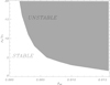 |
Fig. 11. Stability diagram for a bipolar configuration. The gray region corresponds to unstable solutions, while the white region corresponds to stable states. The vertical axis represents the density contrast between the core of the AR and the external environment, while the horizontal axis corresponds to the reference plasma-β, β00. In this plot, we have used a bipole with d = 0.25 and z0 = 0.5 in the domain xmin = −2, xmax = 2, ymin = −2, ymax = 2, zmin = 0, and zmax = 4. The temperature contrast, TAR = 2 TC, is the same for all the points. |
The stable/unstable parameter regions also depend on the size of the computational box since this parameter changes the wavenumbers that fit into the domain (see Eqs. (62)–(64)). Starting from a stable situation and increasing the length of the domain in each direction inevitably leads to an unstable situation because the maximum wavelengths increase. In particular, the wavelength along the magnetic field increases because the field lines are longer in the larger box. The opposite is also true: When starting with an unstable state, by progressively reducing the size of the domain, a stable situation is eventually achieved. This is in qualitative agreement with the behaviour found in Parker’s problem, and it is a characteristic feature of magnetic buoyancy instability.
We also investigated the effect of shear on the stability of the configurations. We have not reported the suppression of the instability by magnetic shear as one would expect for pure interchange modes. This is an additional indication that the instability found in this work is dominated by the undular component of the 3D modes. Nevertheless, we have not considered magnetic structures with a large amount of shear that could have a strong effect on the characteristics of the modes.
9. Discussion and conclusions
We have carried out an initial exploratory study of the application of EPs in 3D to obtain MHS solutions under the presence of gas pressure and gravity that can represent ARs. Due to the nonlinearity of the equilibrium equations, one of the main difficulties in the use of EPs (see Stern 1970) is the calculation of these variables, even when the magnetic field is known. Nevertheless, we have shown that using the potential solution for the magnetic field is a starting point and that the EPs can be numerically calculated when departures from the current-free case are considered. In particular, we used analytical expressions based on an axially symmetric potential configuration as initial distributions of α and β. In addition to the inclusion of the pressure gradient force and the gravitational force, we also incorporated shear in the magnetic field. We investigated different methods and have found that the most efficient procedure is to gradually transform the potential magnetic field at the boundaries of the domain into a non-potential field by applying specific transformations that naturally increase the helicity in the system. This method is effective and transparent and can be viewed as a particular case of other families of transformations that could be investigated in the future.
The choice of the particular functional dependence of gas pressure and temperature on the EPs determines the type of thermal structure of the models. This choice is in principle arbitrary, but based on the typical features of ARs, with hot and dense plasma cores, we have shown that assuming that pressure and temperature are proportional to the square of α (see also Terradas et al. 2022), the basic features of ARs can be reproduced. It is worth noting that α and β can be gauged, and therefore the thermal structure changes according to the specific gauge. Constraints on the gauges need to be imposed based on the observational data. Our models describe the main features of ARs regarding the diffuse background, and in any case, they are not intended to explain the fine structure of coronal loops embedded in ARs, which are most likely due to localised heating.
The three-dimensional configurations under force balance that we numerically computed can be used in the future to study the propagation and interaction of global MHD waves with ARs, i.e. can be used in time-dependent simulations. The interplay of global MHD waves with CHs, which is poorly addressed in the literature due to a lack of 3D models, can also be investigated using the approach proposed in this paper.
Although the topology of the magnetic field must be simple in order to use a description based on EPs (see Sect. 1), we have shown that it is possible to obtain MHS solutions that include null lines under the presence of gas pressure and gravity. These critical points can still be represented using EPs, although we have not investigated geometries with truly 3D null points that may contain spine lines and fan planes and where the description based on EPs fails (see Hesse & Schindler 1988). Even with this limitation, studies about the propagation of waves around null lines can benefit from the models we propose.
We have provided an initial investigation of the stability properties of the numerically computed equilibrium configurations by the application of the sufficient stability criterion established by Zwingmann (1984, 1987) but applied in 3D. An interesting property of the constructed models is that for some values of the parameters (namely, high plasma-β, dense active region cores, and significantly big spatial domains), the system is unstable. For these unstable modes, the magnetic buoyancy force dominates the stabilising effects due to magnetic curvature, magnetic shear, and line-tying, at least in the regime considered in the present work.
Interestingly, the formalism used in the current paper can be extended to the case with pressure and temperature (and therefore density) changing explicitly with height. This model could be used to include, for example, the effect of an idealised chromosphere in the model through the presence of a low temperature and a high density layer. Hence, the method used in this work could be applied not only to the solar corona but also to lower layers in the solar atmosphere, as has been done recently using other approaches by Zhu & Wiegelmann (2018, 2022). In relation to this problem, it is important to mention that the instability criterion applied in this work is only valid when no purely convective instabilities are present. The isothermal case along the magnetic field lines studied in this paper fits into this category, but this does not need to be the case in a more realistic situation, specially if the transition between the chromosphere and corona is included in the models. Nevertheless, studying the stability of an arbitrary non-isothermal 3D configuration is a difficult task that inevitably requires the calculation of the full spectrum of modes through the computation of the MHD eigenmodes. These computations are even more complex when the effect of flows are included in the models. This is a more realistic situation than the static case since there is ubiquitous evidence in the observations of the presence of flows in the solar corona, especially in ARs. As a first step, we could suppose that the flow is field aligned and apply a similar formalism as the one used in the present paper and include additional terms in the equations to account for the flow effect (see further details in Appendix 1 of Schindler 2006).
Finally, it is important to emphasise that the families of equilibria numerically constructed in the present paper cannot be expected to model realistic solar ARs in detail. Though our results are useful as direct demonstration of basic physical effects and as idealised situations, they can still provide some physical insight into more realistic situations. For example, the energy considerations in the AR (radiative losses, thermal conduction, and heating) and the fine structure due to magnetic loops have been completely ignored. But even with the limitations of the approach used in this paper, we argue that the utilisation of EPs to describe ARs is useful and should be investigated in more detail in the future.
Acknowledgments
This publication is part of the R+D+i project PID2020-112791GB-I00, financed by MCIN/AEI/10.13039/501100011033. T.N. acknowledges financial support by the UK’s Science and Technology Facilities Council (STFC) via Consolidated Grants ST/S000402/1 and ST/W001195/1. The authors thank the anonymous referee for useful comments and suggestions that helped to improve the paper.
References
- Aly, J. J. 1989, Sol. Phys., 120, 19 [NASA ADS] [CrossRef] [Google Scholar]
- Atanasiu, C. V., Günter, S., Lackner, K., & Miron, I. G. 2004, Phys. Plasmas, 11, 3510 [NASA ADS] [CrossRef] [Google Scholar]
- Barnes, C. W., & Sturrock, P. A. 1972, ApJ, 174, 659 [NASA ADS] [CrossRef] [Google Scholar]
- Birn, J., & Schindler, K. 1981, in Solar Flare Magnetohydrodynamics, ed. E. R. Priest, 337 [Google Scholar]
- Chandrasekhar, S. 1961, Hydrodynamic and Hydromagnetic Stability (Oxford: Clarendon Press) [Google Scholar]
- Cheng, C. Z. 1995, J. Geophys. Res., 22, 2401 [NASA ADS] [Google Scholar]
- Cheng, C. Z. 2003, J. Geophys. Res. Space Phys., 108, 1002 [NASA ADS] [CrossRef] [Google Scholar]
- Cuperman, S., Ofman, L., & Semel, M. 1989, A&A, 216, 265 [NASA ADS] [Google Scholar]
- Ganesan, S., & Tobiska, L. 2017, Finite Elements: Theory and Algorithms (Cambridge: Cambridge University Press) [CrossRef] [Google Scholar]
- Gary, G. A. 2001, Sol. Phys., 203, 71 [Google Scholar]
- Grad, H. 1964, Phys. Fluids, 7, 1283 [NASA ADS] [CrossRef] [Google Scholar]
- Gradshteyn, I. S., & Ryzhik, I. M. 2007, Table of Integrals, Series, and Products, 7th edn. (Amsterdam: Elsevier/Academic Press), xlviii+1171, translated from the Russian, Translation edited and with a preface by Alan Jeffrey and Daniel Zwillinger, With one CD-ROM (Windows, Macintosh and UNIX) [Google Scholar]
- Hesse, M., & Birn, J. 1993, Adv. Space Res., 13, 249 [NASA ADS] [CrossRef] [Google Scholar]
- Hesse, M., & Schindler, K. 1988, J. Geophys. Res., 93, 5559 [Google Scholar]
- Hood, A. W. 1984, Geophys. Astrophys. Fluid Dyn., 28, 223 [NASA ADS] [CrossRef] [Google Scholar]
- Kabin, K., Rankin, R., Waters, C. L., et al. 2007, Planet. Space Sci., 55, 820 [NASA ADS] [CrossRef] [Google Scholar]
- Kaiser, R., & Salat, A. 1997, J. Plasma Phys., 57, 425 [NASA ADS] [CrossRef] [Google Scholar]
- Kulsrud, R. M. 2004, Plasma Physics for Astrophysics (Princeton: Princeton University Press) [Google Scholar]
- Low, B. C. 1975, ApJ, 197, 251 [NASA ADS] [CrossRef] [Google Scholar]
- Low, B. C. 1980, Sol. Phys., 65, 147 [NASA ADS] [CrossRef] [Google Scholar]
- Low, B. C. 1985, ApJ, 293, 31 [NASA ADS] [CrossRef] [Google Scholar]
- Low, B. C. 1991, ApJ, 370, 427 [NASA ADS] [CrossRef] [Google Scholar]
- Low, B. C. 1992, ApJ, 399, 300 [NASA ADS] [CrossRef] [Google Scholar]
- Low, B. C. 1993a, ApJ, 408, 689 [NASA ADS] [CrossRef] [Google Scholar]
- Low, B. C. 1993b, ApJ, 408, 693 [NASA ADS] [CrossRef] [Google Scholar]
- McKee, C. F., & Zweibel, E. G. 1992, ApJ, 399, 551 [CrossRef] [Google Scholar]
- Neukirch, T. 1993a, J. Geophys. Res., 98, 3753 [NASA ADS] [CrossRef] [Google Scholar]
- Neukirch, T. 1993b, A&A, 274, 319 [NASA ADS] [Google Scholar]
- Neukirch, T. 1995, A&A, 301, 628 [NASA ADS] [Google Scholar]
- Neukirch, T. 1997, A&A, 325, 847 [NASA ADS] [Google Scholar]
- Neukirch, T. 2015, Introduction to the Theory of MHD Equilibria (Charleston: CreateSpace Independent Publishing Platform) [Google Scholar]
- Neukirch, T., & Rastätter, L. 1999, A&A, 348, 1000 [NASA ADS] [Google Scholar]
- Neukirch, T., & Romeou, Z. 2010, Sol. Phys., 261, 87 [NASA ADS] [CrossRef] [Google Scholar]
- Neukirch, T., & Wiegelmann, T. 2019, Sol. Phys., 294, 171 [NASA ADS] [CrossRef] [Google Scholar]
- Parker, E. N. 1966, ApJ, 145, 811 [NASA ADS] [CrossRef] [Google Scholar]
- Parker, E. N. 1979, Cosmical Magnetic Fields. Their Origin and their Activity (Oxford: Clarendon Press) [Google Scholar]
- Parnell, C. E., Smith, J. M., Neukirch, T., & Priest, E. R. 1996, Phys. Plasmas, 3, 759 [NASA ADS] [CrossRef] [Google Scholar]
- Platt, U., & Neukirch, T. 1994, Sol. Phys., 153, 287 [NASA ADS] [CrossRef] [Google Scholar]
- Priest, E., & Forbes, T. 2007, Magnetic Reconnection (New York: Cambridge University Press) [Google Scholar]
- Rankin, R., Kabin, K., & Marchand, R. 2006, Adv. Space Res., 38, 1720 [NASA ADS] [CrossRef] [Google Scholar]
- Roberts, P. 1967, An Introduction to Magnetohydrodynamics (New York: American Elsevier Publishing Co.) [Google Scholar]
- Romeou, Z., & Neukirch, T. 1999, ESA Spec. Publ., 9, 871 [NASA ADS] [Google Scholar]
- Romeou, Z., & Neukirch, T. 2001, in Astrophysics and Space Science Library, eds. A. Hanslmeier, M. Messerotti, & A. Veronig, 259, 303 [NASA ADS] [CrossRef] [Google Scholar]
- Romeou, Z., & Neukirch, T. 2002, J. At. Solar-Terr. Phys., 64, 639 [NASA ADS] [CrossRef] [Google Scholar]
- Rosner, R., Low, B. C., Tsinganos, K., & Berger, M. A. 1989, Geophys. Astrophys. Fluid Dyn., 48, 251 [NASA ADS] [CrossRef] [Google Scholar]
- Schindler, K. 2006, Physics of Space Plasma Activity (Cambridge: Cambridge University Press) [CrossRef] [Google Scholar]
- Schindler, K., Birn, J., & Janicke, L. 1983, Sol. Phys., 87, 103 [NASA ADS] [CrossRef] [Google Scholar]
- Schindler, K., Hesse, M., & Birn, J. 1988, J. Geophys. Res., 93, 5547 [Google Scholar]
- Semel, M. 1988, A&A, 198, 293 [NASA ADS] [Google Scholar]
- Stern, D. P. 1967, J. Geophys. Res., 72, 3995 [NASA ADS] [CrossRef] [Google Scholar]
- Stern, D. P. 1970, Am. J. Phys., 38, 494 [NASA ADS] [CrossRef] [Google Scholar]
- Stern, D. P. 1976, Rev. Geophys. Space Phys., 14, 199 [Google Scholar]
- Stern, D. P. 1994a, J. Geophys. Res., 99, 2443 [NASA ADS] [CrossRef] [Google Scholar]
- Stern, D. P. 1994b, J. Geophys. Res., 99, 17169 [NASA ADS] [CrossRef] [Google Scholar]
- Terradas, J., Soler, R., Oliver, R., et al. 2022, A&A, 660, A136 [NASA ADS] [CrossRef] [EDP Sciences] [Google Scholar]
- Wiegelmann, T., & Sakurai, T. 2021, Liv. Rev. Sol. Phys., 18, 1 [NASA ADS] [CrossRef] [Google Scholar]
- Zaharia, S. 2008, J. Geophys. Res. Space Phys., 113, A08221 [Google Scholar]
- Zaharia, S., Cheng, C., & Maezawa, K. 2004, Ann. Geophys., 22, 251 [NASA ADS] [CrossRef] [Google Scholar]
- Zhu, X., & Wiegelmann, T. 2018, ApJ, 866, 130 [NASA ADS] [CrossRef] [Google Scholar]
- Zhu, X., & Wiegelmann, T. 2022, A&A, 658, A37 [NASA ADS] [CrossRef] [EDP Sciences] [Google Scholar]
- Zhu, X., Neukirch, T., & Wiegelmann, T. 2022, Sci. China Technol. Sci., 65, 1710 [CrossRef] [Google Scholar]
- Zienkiewicz, O. C., Taylor, R. L., & Zhu, J. Z. 2013, The Finite Element Method: Its Basis and Fundamentals (Elsevier) [Google Scholar]
- Zwingmann, W. 1984, PhD Thesis, Ruhr-Universität Bochum, Bochum, Germany [Google Scholar]
- Zwingmann, W. 1987, Sol. Phys., 111, 309 [NASA ADS] [CrossRef] [Google Scholar]
- Zwingmann, W., Schindler, K., & Birn, J. 1985, Sol. Phys., 99, 133 [NASA ADS] [CrossRef] [Google Scholar]
Appendix A: The divergence form of the operator
We present the equilibrium equations given by the PDEs in Eqs. (9)–(10) in divergence form. It is not difficult to show that using the divergence and the gradient operators the equations are
 (A.1)
(A.1)
where C, D, and E are 3 × 3 diagonal matrices, given below. The compact form of the PDEs has some advantages if Neumann BCs are used instead of Dirichlet conditions, which is generally required when the problem is written in weak form (typically necessary when using finite elements).
The matrices that appear in the divergence form of Eq. (A.1) are
 (A.2)
(A.2)
 (A.3)
(A.3)
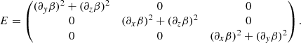 (A.4)
(A.4)
Appendix B: The divergence form of the linearised operator
The linear operator is derived by linearising Eq. (A.1), that is, by assuming that α′ and β′ are small perturbations on the initial equilibrium vales α and β. Using the Taylor expansion of gas pressure around the equilibrium and keeping terms up to the first order in the perturbed quantities, the result, written again in divergence form for completeness, is
 (B.1)
(B.1)
where J is the equilibrium current density given by Eq. (8), while
 (B.2)
(B.2)
and
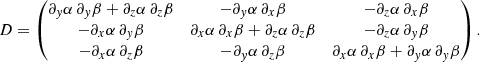 (B.3)
(B.3)
The matrix  is equal to C but with the substitution of β by α, while
  is the same as D but with α and β swapped. The non-divergence form of the linear operator is given in Eq. (2.5) of Zwingmann (1987).
All Figures
|
Fig. 1. Sketch of the bipolar configuration. Potential magnetic field lines (pink curves with arrows) and two magnetic surfaces associated to the EPs α (green color) and β (brown color) for a bipole with d = 0.25 and z0 = 0.5 (all the lengths are hereafter normalised to H). The intersection of the two surfaces, see the yellow curve, represents a particular magnetic field line. The distribution of the vertical component of the magnetic field at z = 0 is represented in gray colors. |
| In the text | |
|
Fig. 2. Potential magnetic field lines and isosurfaces calculated numerically for a non-symmetric case along x-direction. In this example, the following parameters have been used: w1 = w2 = 1/4, z1 = −3/4, z2 = 1, C1 = 1, and C2 = −0.5. |
| In the text | |
|
Fig. 3. Potential magnetic field lines and isosurfaces that include X-points. A visible critical point is located around x = 0.5 and y = 0.5, but due to rotational symmetry, it is repeated along a circular path, and in reality, it is a null line. The same parameters as in Fig. 2 were used except that C1 and C2 have the same sign in this case. |
| In the text | |
|
Fig. 4. Typical mesh structure used in finite element calculations. The x-axis and y-axis point along the orange and green faces of the box, while the z-axis is vertical. A non-uniform grid in each direction has been used to improve the accuracy of the calculations. The most refined region of the grid is located around x = y = z = 0. In this example, the grid has 62 500 elements. |
| In the text | |
|
Fig. 5. Three dimensional bipolar configuration. Magnetic field lines and volume density (normalised to coronal density) for β00 = 1.4 × 10⁻³ (top panel) and for β00 = 1.4 × 10⁻¹ (bottom panel). In this example pAR = 4 pC, TAR = 2 TC, d = 0.25, z0 = 0.1 and αref = α(0, 0, 0). |
| In the text | |
|
Fig. 6. Magnetic field lines and temperature volume for same model as in Fig. 5, bottom panel. Temperature is normalised to 1 MK. |
| In the text | |
|
Fig. 7. Magnetic field lines and plasma-β isosurfaces. The three isosurfaces represent values of 0.1, 0.01, and 0.001 when moving from the exterior to the interior surfaces. This example corresponds to the case shown in Fig. 5, top panel. |
| In the text | |
|
Fig. 8. Non-potential magnetic field lines and magnetic isosurfaces calculated numerically by applying an affine shear transformation on the EPs with sy = 0.6 and sx = sy/4. Gas pressure and gravity are included. In this model, the minimum plasma beta is around 1.4 × 10⁻³, while the maximum is around 2.5, which is well above one. In this example, we used a bipole with d = 0.25 and z0 = 0.5 in the domain xmin = −2, xmax = 2, ymin = −2, ymax = 2, zmin = 0, and zmax = 4. |
| In the text | |
|
Fig. 9. Non-potential magnetic field lines and isosurfaces calculated numerically by applying transformation on EPs using Eq. (51). Gas pressure and gravity are present. Compare with Fig. 2. In this configuration, a0 = 0.6, x0 = 1, w = 1, β00 = 1.4 × 10⁻³, and αref = α(−1, 0, 0). |
| In the text | |
|
Fig. 10. Magnetic field lines and volume density (normalised to the coronal density) for a situation that contains a null line. In this example, magnetic shear with a0 = 0.3, x0 = 1, and w = 1 has been induced in the structure. Gas pressure and gravity are present with β00 = 1.4 × 10⁻³. |
| In the text | |
|
Fig. 11. Stability diagram for a bipolar configuration. The gray region corresponds to unstable solutions, while the white region corresponds to stable states. The vertical axis represents the density contrast between the core of the AR and the external environment, while the horizontal axis corresponds to the reference plasma-β, β00. In this plot, we have used a bipole with d = 0.25 and z0 = 0.5 in the domain xmin = −2, xmax = 2, ymin = −2, ymax = 2, zmin = 0, and zmax = 4. The temperature contrast, TAR = 2 TC, is the same for all the points. |
| In the text | |
Current usage metrics show cumulative count of Article Views (full-text article views including HTML views, PDF and ePub downloads, according to the available data) and Abstracts Views on Vision4Press platform.
Data correspond to usage on the plateform after 2015. The current usage metrics is available 48-96 hours after online publication and is updated daily on week days.
Initial download of the metrics may take a while.