| Issue |
A&A
Volume 671, March 2023
|
|
|---|---|---|
| Article Number | A30 | |
| Number of page(s) | 7 | |
| Section | The Sun and the Heliosphere | |
| DOI | https://doi.org/10.1051/0004-6361/202244599 | |
| Published online | 02 March 2023 | |
Temporal and spatial association between microwaves and type III bursts in the upper corona
1
Institute of Solar-Terrestrial Physics, 126a Lermontov St., Irkutsk 664033, Russia
e-mail: This email address is being protected from spambots. You need JavaScript enabled to view it.
2
Mullard Space Science Laboratory, Department of Space and Climate Physics, University College London, Dorking, UK
e-mail: This email address is being protected from spambots. You need JavaScript enabled to view it.
Received:
26
July
2022
Accepted:
2
January
2023
Abstract
One of the most important tasks in solar physics is the study of particles and energy transfer from the lower corona to the outer layers of the solar atmosphere. The most sensitive methods for detecting fluxes of non-thermal electrons in the solar atmosphere is observing their radio emission using modern large radioheliographs. We analyzed joint observations from the 13 April 2019 event observed by LOw-Frequency ARray (LOFAR) at meter wavelengths, and the Siberian Radio Heliograph (SRH) and the Badary Broadband Microwave Spectropolarimeter (BBMS) spectropolarimeter in microwaves performed at the time of the second PSP perihelion. During a period without signatures of non-thermal energy release in X-ray emission, numerous type III and/or type J bursts were observed. During the same two hours we observed soft X-ray brightenings and the appearance of weak microwave emission in an abnormally narrow band around 6 GHz. At these frequencies the increasing flux is well above the noise level, reaching 9 sfu. In the LOFAR dynamic spectrum of 53−80 MHz a region is found that lasts about an hour whose emission is highly correlated with 6 GHz temporal profile. The flux peaks in the meter waves are well correlated with extreme UV (EUV) emission variations caused by repeated surges from the bright X-point. We argue that there is a common source of non-thermal electrons located in the tail of the active region, where two loop systems of very different sizes interacted. The frequencies of type III and/or type J bursts are in accordance with large loop heights around 400 Mm, obtained by the magnetic field reconstruction. The microwave coherent emission was generated in the low loops identified as bright X-ray points seen in soft X-ray and EUV images, produced by electrons with energies several tens of keV at about twice the plasma frequency.
Key words: Sun: radio radiation / Sun: activity / Sun: X-rays, gamma rays
© The Authors 2023
 Open Access article, published by EDP Sciences, under the terms of the Creative Commons Attribution License (https://creativecommons.org/licenses/by/4.0), which permits unrestricted use, distribution, and reproduction in any medium, provided the original work is properly cited.
This article is published in open access under the Subscribe to Open model. This email address is being protected from spambots. You need JavaScript enabled to view it. to support open access publication.
1. Introduction
One important task connected with the corona heating problem is exploring the physical mechanisms that produce, accelerate, and transport energetic particles in the upper corona. Imaging spectroscopy of meter type III bursts provides us with a powerful tool for diagnostics of non-thermal electron fluxes moving along magnetic lines in the upper corona. Due to the coherent emission mechanism, weak electron beams can produce significant radio flux, and imaging of type III (types J and U bursts) can be use to trace open and closed magnetic flux tubes in the upper corona (e.g., Reid & Kontar 2017a). Since the radiation frequency is proportional to the square root of the local plasma density (Ginzburg & Zhelezniakov 1958), spectral observations make it possible to estimate the height of the emitting structures if the density dependence on height is known.
The spatial and spectral evolution of type III bursts has been studied for many decades (see one of the latest reviews by Reid 2020 and references herein). Mainly, the magnetic connectivity between the sources of meter emission in the upper corona and electron acceleration sites in low corona are studied using the temporal correlation between hard X-ray (HXR) bursts and type III emission (Kane 1972; Aschwanden et al. 1995; Reid et al. 2014; Reid & Vilmer 2017). It was found that type IIIs are commonly associated with jets in extreme ultraviolet (EUV) and X-rays (e.g., Krucker et al. 2011). The results suggest that escaping non-thermal electron events are often associated with the interchange reconnection scenario of energy release when reconnection occurs between open and closed magnetic field lines at heights of 5−10 Mm (Cairns et al. 2018).
Active regions typically emit at meter wave emission during their lifetimes, known as radio noise storms, thought to be associated with non-thermal electrons continuously accelerated to relatively low energies. The small energy release events can be completely silent in observable HXR emission, yet produce type III bursts. For example, type IIIs can be generated even during such faint events as bright points (see the review by Reid et al. 2014). The data on meter bursts were first used by Kundu et al. (1994) as evidence of electron acceleration in the faint energy release processes in the low solar atmosphere.
As a rule, the faint transient events in the low corona and the transition layer are seen in microwaves due to bremsstrahlung of the heated plasma at frequencies above 10 GHz (White et al. 1995). In some events the number and energy of non-thermal electrons accelerated during low C-class flares is sufficient to generate broadband gyrosynchrotron emission. The spectrum overturn frequencies are of several GHz, and there is a response in HXR emission. A recent study with the high-sensitivity 48-antenna Siberian Radio Heliograph (SRH) showed that the main flux contribution is provided by bremsstrahlung and the non-thermal electrons are observed during the first minutes of microflares (Altyntsev et al. 2020).
On the other hand, the most sensitive diagnostics of non-thermal electrons is the coherent radio emission due to the excited plasma turbulence. The long-lasting abnormally narrow band emission in an active region was observed with the high-sensitivity RATAN-600 (Yasnov et al. 2003). The brightness temperature was 2×10⁷ K at frequency 5−6 GHz. The authors suggest that a model with second harmonic emission resulting from the wave–wave coalescence process of two upper-hybrid modes explains the observed spectrum well. The sufficient level of plasma turbulence can be generated by the electrons with pitch-angle anisotropy and energy of several keV (Zaitsev et al. 1997).
Recently, an unusual narrowband radio emission in the 5−7 GHz band originating from the weak X-ray bright point on 13 April 2019 was discussed by Altyntsev et al. (2022). This event was observed during the second Parker Solar Probe perihelion. An analysis showed that characteristics of the spectrum of microwave emission indicated a coherent emission mechanism produced by electrons trapped in low coronal loops. The coherent emission was generated by electrons with energies of several tens of keV at the harmonic of the plasma frequency. In addition, numerous bursts were observed by LOFAR over this time. The goal of this study is to find the response in the upper corona to the X-ray point appearance using the observations of type III and/or J bursts at meter wavelengths.
2. Instrumentation
Coronal type III bursts were recorded by the LOw-Frequency ARray (LOFAR, van Haarlem et al. 2013) in tied-array mode. The observations were made using the LOFAR low-band antenna (LBA) between 80 and 30 MHz with a sub-band width of 0.192 MHz and a time integration of approximately 0.01 s. We then integrated the time resolution to approximately 0.1 s to improve the signal-to-noise ratio.
The solar disk imaging was performed with the 48-antenna prototype of the Siberian Radio Heliograph at five frequencies: 4.5, 5.2, 6.0, 6.8, and 7.5 GHz with 8.4 s time cadence (Lesovoi et al. 2012, 2017). The interferometer maximum base was 107.4 m, and the SRH beamwidth was up to 100 arcsec and varied inversely with frequency. To measure the microwave emission spectrum, we used data of the Badary Broadband Microwave Spectropolarimeter (BBMS; Zhdanov & Zandanov 2011) with a 4−8 GHz range of received frequencies.
To locate soft X-ray (SXR) sources we use data from the X-Ray Telescope (XRT; Golub et al. 2007) on Hinode (Kosugi et al. 2007). The XRT is sensitive in the energy band from ∼0.15 to more than 3 keV and can detect emission from plasma with temperatures from ∼1 MK to several tens of MK.
Data on spectral and spatial characteristics of EUV emission lines were obtained at the Solar Dynamics Observatory (SDO; Pesnell et al. 2012). Images of the full solar disk were recorded every 12 s with the Atmospheric Imaging Assembly (AIA; Lemen et al. 2012) with 0.6 arcsec resolution. In our work, we used vector magnetograms obtained with the Helioseismic and Magnetic Imager (HMI; Scherrer et al. 2012; Schou et al. 2012) aboard the Solar Dynamics Observatory.
3. Observations
Co-temporal dynamical spectra of radio emission recorded on 13 April 2019 in meter and microwave waves are shown in Fig. 1. The numerous short bursts cover the receiving band of the LOFAR (panel a) during the interval 05:43:30−07:39:59 of common observations with the BBMS spectropolarimeter. Panel b presents the dynamic spectrum recorded by the BBMS in the microwave range 4−8 GHz. To highlight radiation brightenings, the quiet Sun emission was excluded in the dynamic spectrum. There are two reliable brightness enhancements up to 9 sfu at frequencies 4.5−7.5 GHz. The duration of these brightenings is 15−20 min. There are also brightness enhancements at frequencies above 7.5 GHz starting at 06:40 and lasting up to the end of the common observations. An inspection of the meter and microwave panels shows that the first enhancement around 6 GHz can be correlated with an emission activity at a high-frequency part of the meter dynamic spectrum, and the second can be linked with meter emission increase in the low-frequency part of the spectrum.
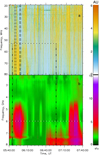 |
Fig. 1. Dynamic spectra on 13 April 2019, recorded by LOFAR (a) and BBMS in microwaves (b). The box in panel (a) with the bounds at 05:45:15 and 06:56:40 gives the spectrum region for which there is a high cross-correlation coefficient with the microwave emission at 6 GHz. The vertical dash-dotted, dashed, and dotted lines indicate the three time intervals used in Fig. 4. The vertical dash-three-dotted lines restrict the time interval for which the highest correlation coefficient was found. |
At the beginning of the first brightness enhancement, the SRH images at 6.25 GHz were available, allowing the localization of the emission source in the lower corona. It was shown by Altyntsev et al. (2022) that the first microwave brightening was generated by non-thermal electrons trapped in the short low coronal loop seen in the soft X-rays as a coronal X-point. The microwave flux is weak, but is sufficient to measure the spectrum at the peak of 6 GHz temporal profile (Fig. 2). The background emission at 05:45 is subtracted here. The microwave spectrum is unusually narrow with a band of 6 ± 1 GHz with very steep slopes at low and high frequencies. The narrowness of the microwave spectrum indicates a non-thermal radiation mechanism.
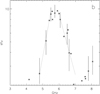 |
Fig. 2. Microwave spectrum calculated as the difference between spectra at 05:45 and 05:58. The bars show the level of noise on the flux profiles. |
Temporal profiles of meter and microwave radiation differ significantly in variability on small timescales (Fig. 3a). It is seen that the microwave profile is smooth in comparison with the meter profile. Thus, the response to microwave-emitting electron fluxes is not related to the intensity of individual meter bursts, rather to the frequency of their repetition. To find whether the electron acceleration in the vicinity of the X-ray coronal point contributed to the generation of the meter bursts, we performed a cross-correlation analysis between profiles of 6 GHz emission and of the frequency-averaged dynamic spectrum over the LOFAR receiving bandwidth. For the analysis we used the profile smoothing with a 1 min window in both frequency ranges. The cross-correlation coefficient calculated for the whole interval of the LOFAR observation is ∼0.35. To locate the time-frequency region with the highest temporal similarity to the 6 GHz profile, we decreased successively the time interval and frequency range of the LOFAR dynamic spectrum used for the cross-correlation calculations. In this way we found a frequency-time region of the meter dynamic spectrum, where the cross-correlation of the frequency-average spectrum profile of this region with the corresponding 6 GHz profile has an extreme whose value reaches 0.72.
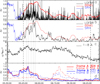 |
Fig. 3. Profiles for time interval (bounded by vertical dashed lines) for which the cross-correlation coefficient between meter and microwave emission reaches 0.72. (a) Flux at 6 GHz (normalized, red curve) and time dependence of the meter flux, integrated over the frequency range 71 ± 0.5 MHz (black solid line). Before 05:45:15 the SRH correlation (blue curve) is shown. (b) Same, but for the meter flux, integrated over frequency range 53−80 MHz (black solid line). The 1 min smoothing window is used. (c) 1−8 Å GOES channel (solid curve), smoothing with 10 s window. (d) 304 Å profile (red solid line) and 171 Å profile (blue solid line) of the emissions summed over the pink frame and over the green frame (dash-dotted and dashed lines) in Fig. 5b. |
The best similarity is thus achieved for the LOFAR dynamic spectrum restricted by the frequency range 53−80 MHz and during the interval from 05:45:15 till 06:48:10. This region is indicated by the box in Fig. 1a. The cross-correlation coefficient of the LOFAR selected box with an average microwave profile over the range of 5−7 GHz is also high and exceeds 0.7. The high cross-correlation suggests a common origin of a large part of the electron population that generates the radio emission in the lower and upper corona. Calculations of the cross-correlation between the 6 GHz profile and profiles at individual LOFAR frequencies show that the coefficient is at a maximum of 0.82 at about 70 MHz and rapidly drops at frequencies below 50 MHz. In addition, the cross-correlation coefficient depends on the degree of smoothing of the meter emission profile. It grows rapidly with an increase in smoothing length up to 1 min, and then its value remains almost constant.
Each individual burst lasts 2−5 s and they occur at a rate of 3−15 per min. In the first part of the selected time interval, brightenings are observed in the beginning of both dynamic spectra, and the frequency about 50 MHz corresponds to the low-frequency boundary in the bright region in the meter dynamic spectrum. To show the properties of the meter bursts, the spectra are shown in two-minute intervals around the maximum intensity in microwaves and at the time of meter wave emission (Fig. 4). The trajectories of drifting bursts in the first interval (panel a) show that there are a number of type III bursts drifting from 70 to 80 MHz down about 50 MHz and indicating the appearance of unstable electron beams propagating into the upper corona. The drift rate of bursts is around 10 MHz s−1 and the type III bursts occur every several seconds. The abrupt stop of the radio bursts at frequencies below 50 MHz strongly indicates the existence of J-bursts, where the exciting electron beam reaches the highest altitude of a closed magnetic structure and stops producing radio emission (Haddock 1959; Takakura & Kai 1966; Ledenev 2008; Reid & Kontar 2017b). At late times of the selected spectral box, meter bursts occur less frequently, and J-type bursts with frequencies down to 50−60 MHz are observed. The J-bursts are observed at lower frequencies later (panel c), when the meter bursts occur at only a few times per minute.
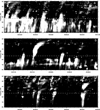 |
Fig. 4. Extended meter dynamic spectra at two-minute intervals indicated by the vertical dash-dotted, dashed, and dotted lines in Fig. 1a. The horizontal dashed lines show the frequency bound of the selected box. |
The time profile at 6 GHz, measured with the SRH (blue curve, until 05:45:15) and BBMS (red), and the LOFAR profile averaged over the selected spectrum region are shown in Fig. 3b. The bounds of the interval with the high cross-correlation coefficient are shown by the dashed lines. In Fig. 3, the vertical dotted lines mark the prominent peaks on the LOFAR profile, which correspond to an increase in the occurrence of type III and/or J bursts. Flux enhancements lasting about 15 min are observed at the beginning of the interval in both frequency ranges. Afterward the intensities gradually subside and experience small enhancements with a period of about 15 min. As follows from Figs. 3a and b, the frequency of occurrence and the intensity of meter bursts grow together with the growth of microwave radiation. However, the microwave radiation profile is smoother and decays more slowly. This behavior indicates that with the general origin of accelerated electrons, microwave radiation is generated not by electron beams during their propagation, but by electrons captured in magnetic loops.
During this interval there are the co-temporal enhancements in the soft GOES flux (Fig. 3c). However, there was no noticeable responses in the GOES 0.5−4 Å channel and the hard X-ray emission recorded by the Fermi Gamma-ray Burst Monitor (Meegan et al. 2009). In the following we concentrate our study on the interval with the first soft X-ray enhancement and the more intensive radio emission.
There is one active region (NOAA 12738) on the solar disk (Fig. 5a) on 13 April 2019. The LOFAR imaging confirms that this active region can be the source of electron fluxes generating the meter bursts. The event was observed in the morning by LOFAR, causing the LOFAR angular diagram to have a relatively wide beam. Moreover, the apparent position of the source on the solar disk is significantly affected by the electromagnetic wave refraction in the Earth’s ionosphere. Therefore, the contours are plotted at 06:48 when the Sun is higher in the sky. These circumstances do not make it possible to precisely locate the injection position of accelerated electrons into the upper corona.
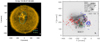 |
Fig. 5. Images on 13 April 2019. (a) Solar disk at 171 Å (SDO/AIA) and contours of brightness temperature at 50, 60, 70 MHz at half height at 06:48; (b) AR 12635 in soft X-rays (XRT/Hinode) at 06:04 and 06:24 (box in the upper right corner) together with the line of sight magnetic field component (±100, ±300, ±1000, ±1500 G). Red and blue contours show positive and negative components, respectively. White contours at (0.2, 0.5, 0.9)×0.6 MK corresponds to brightness temperature at 6.25 GHz (SRH) in intensity at 05:44:49. The SRH beam width is 52×35 arcsec. Black solid and dashed contours indicate the brightness temperature in the right and left polarization, respectively. The levels are (0.5, 0.7)×2.8×104 K and −(0.7, 0.5)×1.6×105 K. The pink and green frames bound the frames for the 171 Å and 304 Å profiles in Fig. 3c. |
The magnetic structure of the active region consists of a large leading S-polarity sunspot and a mixture of small magnetic patches of different signs, distributed over the trailing part of the region (Fig. 5b). The two temporary brightenings of soft X-ray radiation, seen on the light curves in Fig. 3c, allows us to localize their sources using the Hinode/XRT imaging. There are loops of different sizes and two bright patches A and B at the times of the soft X-ray brightening. The Be-thin images at 06:04 and 06:24 show that the structure of the SXR sources does not change in time other than at these two patches. Patch A includes a short loop with distance of ∼20 arcsec between the footpoints and width of ∼4 arcsec, which is the brightest X-ray source during the first soft X-ray increase. Therefore, we believe that the main energy release source is located near patch A at this time. During the second increase, patch A became faint and patch B became brighter (see the box in the upper right corner of Fig. 5b).
The microwave images at 6.25 GHz in intensity and polarization were available during the first enhancement up to 05:44:49. In intensity and left-hand polarization the brightness temperature contours cover the main sunspot, but the weakest intensity contour is shifted toward patch A. In the right polarization there are two sources at the footpoints of the large loops. In patch A the polarization degree reaches 30%. The northeastern right polarized source coincides with loop A. Thus, this place corresponds to the source of the non-thermal microwave emission in the low corona.
The temporal dependences of the 171 Å and 304 Å fluxes summed over the frames around patches A and B are shown by the blue and red curves in Fig. 3d. There are also two intensity enhancements co-temporal with the soft X-ray profile (panel c). Patch A is bright during the first enhancement only (solid curves), but the EUV emission in patch B increases mainly at the second soft X-ray enhancements. We note that during the second brightening the relative flux of low-energy radiation in the He II line increases relative to the flux in the Fe IX line. Thus, the energy release process is weaker in patch B.
The EUV images were considered by Altyntsev et al. (2022). They were seen as short filaments at patch A with the X-ray loop. During the interval under study, some filaments repeatedly erupted and provided the three peaks of 171 Å emission. The high temporal correspondence of these peaks in the LOFAR and EUV curves in Figs. 3a, b, and d shows that the emitting electrons escape to the upper corona from the vicinity of the bright point A. During the last marked peaks of meter radiation, the flux from patch A is relatively high, but the co-temporal EUV peaks do not stand out noticeably.
4. Discussion
The high sensitivity of the LOFAR radio telescope made it possible to record a series of drifting bursts during the period without signatures of electron acceleration in X-ray emission. In these two-hour common observations with the SRH, signatures of electron acceleration in the low corona have also been found in the microwave emission. We were unable to find corresponding radio bursts in intermediate frequency observations, perhaps due to the lack of sensitivity of available facilities such as the Culgoora and Learmonth spectrographs.
Another interpretation could be due to microwave emissions and coherent metric emissions being produced by electrons accelerated in multiple reconnection sites connected by common magnetic field lines. In this case the reconnection in low-lying loops will produce energetic electrons responsible for the microwave radiation, but can also trigger a secondary reconnection at higher altitude responsible for the type III and/or J producing electron beams (see, e.g., Benz et al. 2005).
Altyntsev et al. (2022) show that the microwave emission in the band 5−7 GHz was generated by a relatively small number of accelerated electrons, trapped in the loop, linked with bright X-ray point A. Their X-ray radiation was below the sensitivity thresholds of the 0.5−4 Å GOES channel and FERMI sensors. The observed intensity and narrow band of the spectrum can be provided by coherent emission from electrons with energies above several tens of keV at the second harmonic plasma frequency, due to the excitation of upper hybrid waves in the loop through pitch-angle anisotropy of non-thermal electrons. This mechanism was proposed by Zaitsev et al. (1997) and was used for the interpretation of the decimetric long-term emission of active region by Yasnov et al. (2003).
It was found that an increase in the occurrence rate of meter bursts in the band 53−80 MHz was highly correlated with the microwave temporal behavior and is caused by long-term energy release near the bright X-ray point A. The peculiarity of this point follows from the calculations of the neutral line of the radial magnetic field component at the different layers above the photosphere (Altyntsev et al. 2022). Small-scale magnetic patches with mixed polarity disappear with height, while the inclusion of the positive polarity near the eastern footpoint of loop A and about 20 arcsec eastward from the major negative sunspot remains clearly distinguishable up to 6 Mm. Between 6 and 9 Mm it becomes completely overlapped by negative polarity, indicating the presence of a null point in this region and possibility of reconnection. A similar magnetic configuration occurs in the vicinity of point B, which brightens in soft X-rays and EUV emission later but does not provide a large increase in type III burst activity in the meter wavelengths. In case B a negative magnetic inclusion is located amid dominating positive magnetic polarity. The magnetic flux anchored to the inclusion has more scattered structure, and its traces disappear at the height of 3 Mm.
Figure 6a represents the configurations of magnetic field lines anchored near points A and B. The configurations are calculated in a potential-field approximation for a uniform grid of [250×400×250] (length, width, height) nodes with a spatial resolution of 1 Mm. SDO/HMI vector magnetogram for 13 April 2019, 5:48 UT was used as input boundary conditions. Pi-ambiguity was removed using the method by Rudenko & Anfinogentov (2014). To study the magnetic field structure around the positive polarity inclusion and the bright XRT loop we assumed local non-potentiality of the magnetic field and performed a nonlinear force-free field (NLFFF) reconstruction in the small subvolume (30×30×4 Mm) near point A (purple lines in Fig. 6a). For this purpose we utilized the optimization method developed by Wheatland et al. (2000) in the implementation by Rudenko & Myshyakov (2009). During the interval under study there were no notable changes in the magnetic configuration.
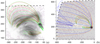 |
Fig. 6. Reconstruction of magnetic structure of AR 12635 in higher (a) and lower (b) spatial resolution. The thick dashed line circumscribes the computational domain. The violet contours represent a neutral line at a height of 1 Mm (a) and 3 Mm (b). The gray background is the soft X-ray image at 06:04 UT (a) and the radial component of the photosphere magnetic field (b). The XRT image was displaced by 20 arcsec to the east and 15 arcsec to the south. |
Potential-field extrapolation reveals that magnetic configurations in the vicinity of points A and B have a similar topology. In each case the small-scale magnetic flux, anchored to the magnetic inclusion, is overlapped by the relatively large-scale magnetic flux (traced by red and green lines in Fig. 6a), anchored to the surrounding magnetic polarity. Small-scale magnetic field lines near point A obtained in the NLFFF approximation (colored in purple) correspond to the bright feature in the XRT image.
Figure 6b represents magnetic field lines of the large-scale potential-field configuration, computed in spherical geometry for a uniform grid with a spatial resolution of 3 Mm. The physical size of the computational domain is 700×700 Mm on the photosphere with a height of 700 Mm. The blue lines anchored near the eastern footpoint of the A loop have a height of up to 400 Mm, comparable to height estimates of type III and/or J-bursts at frequencies down to 50 MHz (e.g., the lower end of the coronal loops in Reid & Kontar 2017a). Brown field lines are connected to the upper boundary of the computational domain, and are therefore considered open field lines.
The vertical components of the magnetic field vectors of the large and small loops are anti-parallel at closely spaced regions, which creates favorable conditions for magnetic reconnection. This is referred to as “interchange reconnection” if a field line that is open to interplanetary space switches the location of its photospheric footpoint (Cairns et al. 2018). The continuous reconnection occurs in the current sheet that forms between the new and old flux. In the reconnection process, the plasma density increases and plasma particles are accelerated by electric fields. Post-reconnection field lines take the shape of a small hot loop and field lines that are open to interplanetary space. Observations show that such magnetic reconfigurations can repeatedly occur due to mini-filament eruptions. Similar repetitive rising filaments have been observed in UV image sequences (Sterling et al. 2015). In the vicinity of point B, where the burst of soft X-ray and ultraviolet radiation was observed about 20 min after the burst at point A, the formation of short eruptive loops was not observed.
5. Conclusion
As part of ground support for the Parker Solar Probe space mission, a long series of observations were carried out by LOFAR during periods of low solar activity. It is shown that the electron source of a series of type III and/or J bursts in the frequency range 50−80 MHz is the interaction of two loop systems with significantly different lengths. The common base of the loops is rooted at the location where small-scale opposite polarity magnetic patches mix and close to the larger dominant polarity. Accelerated electrons then move along large loops with a radius of the order of the Sun’s radius, and are emitting in the meter range due to coherent plasma emission. Microwave emission can be generated by other parts of the non-thermal electrons in the low loops. The spectrum of microwave emission is abnormally narrow and indicates a non-thermal origin. Thus, the use of large multiwave radioheliographs makes it possible to reveal non-thermal processes in the solar corona not only in weak flares, but also in transient events. The combination of cross-correlation analysis of the temporal profiles of radio emission from the lower and upper corona with the localization of sources makes it possible to verify the methods of reconstruction of coronal magnetic fields.
Acknowledgments
We thank the anonymous referee for his very important and useful comments which helped to improve this paper. This study was supported by the Russian project of RFBR No. 21-52-10012. H. Reid acknowledges funding from the STFC Consolidated Grant ST/W001004/1. The development of the methods used in Sect. 3 was financially supported by the Ministry of Science and Higher Education of the Russian Federation. The SRH and BBMS data were obtained using the Unique Research Facility Siberian Solar Radio Telescope (http://ckp-angara.iszf.irk.ru/index_en.html). We are grateful to the teams of the Siberian Radio Heliograph, Nobeyama Radio Observatory, LOFAR, SDO, RHESSI, FERMI who have provided open access to their data. This paper is based (in part) on data obtained with the International LOFAR Telescope (ILT) under project code L701901. LOFAR (van Haarlem et al. 2013) is the Low Frequency Array designed and constructed by ASTRON. It has observing, data processing, and data storage facilities in several countries, that are owned by various parties (each with their own funding sources), and that are collectively operated by the ILT foundation under a joint scientific policy. The ILT resources have benefitted from the following recent major funding sources: CNRS-INSU, Observatoire de Paris and Universite d’Orleans, France; BMBF, MIWF-NRW, MPG, Germany; Science Foundation Ireland (SFI), Department of Business, Enterprise and Innovation (DBEI), Ireland; NWO, The Netherlands; The Science and Technology Facilities Council, UK; Ministry of Science and Higher Education, Poland.
References
- Altyntsev, A. T., Meshalkina, N. S., Fedotova, A. Y., & Myshyakov, I. I. 2020, ApJ, 905, 149 [NASA ADS] [CrossRef] [Google Scholar]
- Altyntsev, A., Meshalkina, N., & Myshyakov, I. 2022, Solar-Terr. Phys., 8, 3 [NASA ADS] [Google Scholar]
- Aschwanden, M. J., Benz, A. O., Dennis, B. R., & Schwartz, R. A. 1995, ApJ, 455, 347 [NASA ADS] [CrossRef] [Google Scholar]
- Benz, A. O., Grigis, P. C., Csillaghy, A., & Saint-Hilaire, P. 2005, Sol. Phys., 226, 121 [NASA ADS] [CrossRef] [Google Scholar]
- Cairns, I. H., Lobzin, V. V., Donea, A., et al. 2018, Sci. Rep., 8, 1676 [NASA ADS] [CrossRef] [Google Scholar]
- Ginzburg, V. L., & Zhelezniakov, V. V. 1958, Sov. Astron., 2, 653 [Google Scholar]
- Golub, L., Deluca, E., Austin, G., et al. 2007, Sol. Phys., 243, 63 [NASA ADS] [CrossRef] [Google Scholar]
- Haddock, F. T. 1959, in URSI Symp. 1: Paris Symposium on Radio Astronomy, ed. R. N. Bracewell, 9, 188 [NASA ADS] [Google Scholar]
- Kane, S. R. 1972, Sol. Phys., 27, 174 [NASA ADS] [CrossRef] [Google Scholar]
- Kosugi, T., Matsuzaki, K., Sakao, T., et al. 2007, Sol. Phys., 243, 3 [Google Scholar]
- Krucker, S., Kontar, E. P., Christe, S., Glesener, L., & Lin, R. P. 2011, ApJ, 742, 82 [Google Scholar]
- Kundu, M. R., Shibasaki, K., Enome, S., & Nitta, N. 1994, ApJ, 431, L155 [NASA ADS] [CrossRef] [Google Scholar]
- Ledenev, V. G. 2008, Sol. Phys., 253, 191 [NASA ADS] [CrossRef] [Google Scholar]
- Lemen, J. R., Title, A. M., Akin, D. J., et al. 2012, Sol. Phys., 275, 17 [Google Scholar]
- Lesovoi, S. V., Altyntsev, A. T., Ivanov, E. F., & Gubin, A. V. 2012, Sol. Phys., 280, 651 [NASA ADS] [CrossRef] [Google Scholar]
- Lesovoi, S., Altyntsev, A., Kochanov, A., et al. 2017, Solar-Terr. Phys., 3, 3 [NASA ADS] [Google Scholar]
- Meegan, C., Lichti, G., Bhat, P. N., et al. 2009, ApJ, 702, 791 [Google Scholar]
- Pesnell, W. D., Thompson, B. J., & Chamberlin, P. C. 2012, Sol. Phys., 275, 3 [Google Scholar]
- Reid, H. A. S. 2020, Front. Astron. Space Sci., 7, 56 [NASA ADS] [CrossRef] [Google Scholar]
- Reid, H. A. S., & Kontar, E. P. 2017a, A&A, 606, A141 [NASA ADS] [CrossRef] [EDP Sciences] [Google Scholar]
- Reid, H. A. S., & Kontar, E. P. 2017b, A&A, 598, A44 [NASA ADS] [CrossRef] [EDP Sciences] [Google Scholar]
- Reid, H. A. S., & Vilmer, N. 2017, A&A, 597, A77 [NASA ADS] [CrossRef] [EDP Sciences] [Google Scholar]
- Reid, H. A. S., Vilmer, N., & Kontar, E. P. 2014, A&A, 567, A85 [NASA ADS] [CrossRef] [EDP Sciences] [Google Scholar]
- Rudenko, G. V., & Anfinogentov, S. A. 2014, Sol. Phys., 289, 1499 [NASA ADS] [CrossRef] [Google Scholar]
- Rudenko, G. V., & Myshyakov, I. I. 2009, Sol. Phys., 257, 287 [NASA ADS] [CrossRef] [Google Scholar]
- Scherrer, P. H., Schou, J., Bush, R. I., et al. 2012, Sol. Phys., 275, 207 [Google Scholar]
- Schou, J., Scherrer, P. H., Bush, R. I., et al. 2012, Sol. Phys., 275, 229 [Google Scholar]
- Sterling, A. C., Moore, R. L., Falconer, D. A., & Adams, M. 2015, Nature, 523, 437 [NASA ADS] [CrossRef] [Google Scholar]
- Takakura, T., & Kai, K. 1966, PASJ, 18, 57 [NASA ADS] [Google Scholar]
- van Haarlem, M. P., Wise, M. W., Gunst, A. W., et al. 2013, A&A, 556, A2 [NASA ADS] [CrossRef] [EDP Sciences] [Google Scholar]
- Wheatland, M. S., Sturrock, P. A., & Roumeliotis, G. 2000, ApJ, 540, 1150 [Google Scholar]
- White, S. M., Kundu, M. R., Shimizu, T., Shibasaki, K., & Enome, S. 1995, ApJ, 450, 435 [NASA ADS] [CrossRef] [Google Scholar]
- Yasnov, L. V., Bogod, V. M., Fu, Q., & Yan, Y. 2003, Sol. Phys., 215, 343 [NASA ADS] [CrossRef] [Google Scholar]
- Zaitsev, V. V., Kruger, A., Hildebrandt, J., & Kliem, B. 1997, A&A, 328, 390 [NASA ADS] [Google Scholar]
- Zhdanov, D. A., & Zandanov, V. G. 2011, Cent. Eur. Astrophys. Bull., 35, 223 [Google Scholar]
All Figures
|
Fig. 1. Dynamic spectra on 13 April 2019, recorded by LOFAR (a) and BBMS in microwaves (b). The box in panel (a) with the bounds at 05:45:15 and 06:56:40 gives the spectrum region for which there is a high cross-correlation coefficient with the microwave emission at 6 GHz. The vertical dash-dotted, dashed, and dotted lines indicate the three time intervals used in Fig. 4. The vertical dash-three-dotted lines restrict the time interval for which the highest correlation coefficient was found. |
| In the text | |
|
Fig. 2. Microwave spectrum calculated as the difference between spectra at 05:45 and 05:58. The bars show the level of noise on the flux profiles. |
| In the text | |
|
Fig. 3. Profiles for time interval (bounded by vertical dashed lines) for which the cross-correlation coefficient between meter and microwave emission reaches 0.72. (a) Flux at 6 GHz (normalized, red curve) and time dependence of the meter flux, integrated over the frequency range 71 ± 0.5 MHz (black solid line). Before 05:45:15 the SRH correlation (blue curve) is shown. (b) Same, but for the meter flux, integrated over frequency range 53−80 MHz (black solid line). The 1 min smoothing window is used. (c) 1−8 Å GOES channel (solid curve), smoothing with 10 s window. (d) 304 Å profile (red solid line) and 171 Å profile (blue solid line) of the emissions summed over the pink frame and over the green frame (dash-dotted and dashed lines) in Fig. 5b. |
| In the text | |
|
Fig. 4. Extended meter dynamic spectra at two-minute intervals indicated by the vertical dash-dotted, dashed, and dotted lines in Fig. 1a. The horizontal dashed lines show the frequency bound of the selected box. |
| In the text | |
|
Fig. 5. Images on 13 April 2019. (a) Solar disk at 171 Å (SDO/AIA) and contours of brightness temperature at 50, 60, 70 MHz at half height at 06:48; (b) AR 12635 in soft X-rays (XRT/Hinode) at 06:04 and 06:24 (box in the upper right corner) together with the line of sight magnetic field component (±100, ±300, ±1000, ±1500 G). Red and blue contours show positive and negative components, respectively. White contours at (0.2, 0.5, 0.9)×0.6 MK corresponds to brightness temperature at 6.25 GHz (SRH) in intensity at 05:44:49. The SRH beam width is 52×35 arcsec. Black solid and dashed contours indicate the brightness temperature in the right and left polarization, respectively. The levels are (0.5, 0.7)×2.8×104 K and −(0.7, 0.5)×1.6×105 K. The pink and green frames bound the frames for the 171 Å and 304 Å profiles in Fig. 3c. |
| In the text | |
|
Fig. 6. Reconstruction of magnetic structure of AR 12635 in higher (a) and lower (b) spatial resolution. The thick dashed line circumscribes the computational domain. The violet contours represent a neutral line at a height of 1 Mm (a) and 3 Mm (b). The gray background is the soft X-ray image at 06:04 UT (a) and the radial component of the photosphere magnetic field (b). The XRT image was displaced by 20 arcsec to the east and 15 arcsec to the south. |
| In the text | |
Current usage metrics show cumulative count of Article Views (full-text article views including HTML views, PDF and ePub downloads, according to the available data) and Abstracts Views on Vision4Press platform.
Data correspond to usage on the plateform after 2015. The current usage metrics is available 48-96 hours after online publication and is updated daily on week days.
Initial download of the metrics may take a while.