| Issue |
A&A
Volume 671, March 2023
|
|
|---|---|---|
| Article Number | A142 | |
| Number of page(s) | 18 | |
| Section | Extragalactic astronomy | |
| DOI | https://doi.org/10.1051/0004-6361/202244597 | |
| Published online | 16 March 2023 | |
MUSE crowded field 3D spectroscopy in NGC 300
IV. Planetary nebula luminosity function⋆
1
Leibniz-Institut für Astrophysik Potsdam (AIP), An der Sternwarte 16, 14482 Potsdam, Germany
e-mail: asoemitro@aip.de
2
Institut für Physik und Astronomie, Universität Potsdam, Karl-Liebknecht-Str. 24/25, 14476 Potsdam, Germany
3
Department of Astronomy & Astrophysics, The Pennsylvania State University, University Park, PA 16802, USA
4
Institute for Gravitation and the Cosmos, The Pennsylvania State University, University Park, PA 16802, USA
5
NSF’s NOIRLab, 950 N. Cherry Ave., Tucson, AZ 85719, USA
6
Leiden Observatory, Leiden University, PO Box 9513 2300 RA Leiden, The Netherlands
Received:
25
July
2022
Accepted:
5
January
2023
Aims. We perform a deep survey of planetary nebulae (PNe) in the spiral galaxy NGC 300 to construct its planetary nebula luminosity function (PNLF). We aim to derive the distance using the PNLF and to probe the characteristics of the most luminous PNe.
Methods. We analysed 44 fields observed with MUSE at the VLT, covering a total area of ∼11 kpc2. We find [O III]λ5007 sources using the differential emission line filter (DELF) technique. We identified PNe through spectral classification with the aid of the BPT diagram. The PNLF distance was derived using the maximum likelihood estimation technique. For the more luminous PNe, we also measured their extinction using the Balmer decrement. We estimated the luminosity and effective temperature of the central stars of the luminous PNe based on estimates of the excitation class and the assumption of optically thick nebulae.
Results. We identify 107 PNe and derive a most-likely distance modulus  (
( Mpc). We find that the PNe at the PNLF cutoff exhibit relatively low extinction, with some high-extinction cases caused by local dust lanes. We present the lower limit luminosities and effective temperatures of the central stars for some of the brighter PNe. We also identify a few Type I PNe that come from a young population with progenitor masses > 2.5 M⊙ but do not populate the PNLF cutoff.
Conclusions. The spatial resolution and spectral information of MUSE allow precise PN classification and photometry. These capabilities also enable us to resolve possible contamination by diffuse gas and dust, improving the accuracy of the PNLF distance to NGC 300.
Key words: galaxies: stellar content / planetary nebulae: general / galaxies: luminosity function / mass function / distance scale / stars: AGB and post-AGB
Full Table D.1 is only available at the CDS via anonymous ftp to cdsarc.cds.unistra.fr (130.79.128.5) or via https://cdsarc.cds.unistra.fr/viz-bin/cat/J/A+A/671/A142
© The Authors 2023
 Open Access article, published by EDP Sciences, under the terms of the Creative Commons Attribution License (https://creativecommons.org/licenses/by/4.0), which permits unrestricted use, distribution, and reproduction in any medium, provided the original work is properly cited.
This article is published in open access under the Subscribe to Open model. Subscribe to A&A to support open access publication.
1. Introduction
The planetary nebula luminosity function (PNLF) is a distance determination method with a precision and accuracy that is comparable to those of the tip of the red giant branch (TRGB) and Cepheid methods (Jacoby 1989; Ciardullo et al. 1989; Ciardullo 2010, 2012; Roth et al. 2021). Using evidence from narrow-band photometric surveys in [O III]λ5007, Ciardullo et al. (1989) showed that the magnitude distribution of planetary nebulae (PNe) for a given galaxy follows an empirical power law defined as

where the brightest PN at the cutoff has an absolute magnitude of M* = −4.53 ± 0.06 with a possible minor dependence on metallicity (Jacoby 1989; Dopita et al. 1992; Ciardullo et al. 2002; Ciardullo 2012). While a number of different formulations have been developed to model the various shapes of the PNLF at fainter magnitudes (Rodríguez-González et al. 2015; Longobardi et al. 2013; Bhattacharya et al. 2019, 2021), such faint-end variations do not affect the definition of the PNLF’s bright-end cutoff, which is the critical feature for distance determinations (Spriggs et al. 2021; Ciardullo 2022).
Until the early 2010s, most PNLF distance measurements were obtained using 4-metre-class telescopes and narrow-band interference filters, and as a result, the method has traditionally been limited to distances of ∼20 Mpc (Jacoby et al. 1990; Ciardullo 2010, 2012, 2022). Although 8-metre-class telescopes were available and even observed PNe at the Coma cluster (∼100 Mpc; Gerhard et al. 2005), most of the instruments had wider bandpass filters, which increased the inclusion of the sky background signal. This limited the PN detection sensitivity, and a high sensitivity is necessary to significantly improve the distance range of the PNLF (Ciardullo 2022). This situation has now changed due to the use of the Multi Unit Spectroscopic Explorer (MUSE; Bacon et al. 2010) integral-field spectrograph on the 8.2-metre Very Large Telescope (VLT) to survey PNe in distant systems (Spriggs et al. 2020, 2021; Roth et al. 2021; Scheuermann et al. 2022). In fact, Roth et al. (2021) have shown that, by using the differential emission line filter (DELF) technique on MUSE data, PNLF measurements are now possible out to distances of ∼40 Mpc under excellent seeing conditions and with the aid of the adaptive optics system. This is mainly due to the narrow effective bandpass of MUSE, which is five times narrower than typical narrow-band filters; this can substantially suppress the background sky noise (Roth et al. 2021).
Previous PNLF studies of late-type galaxies using [O III]λ5007 narrow-band filters were also hampered by the possible confusion with supernova remnants (SNRs) or H II regions (Herrmann et al. 2008; Herrmann & Ciardullo 2009; Frew & Parker 2010). While Hα narrow-band imaging allows the exclusion of H II regions, it cannot be used to exclude SNRs, whose classification typically relies on the [S II]λ6716, 6731 lines. In M31 and M33, Davis et al. (2018a) found that the SNR contamination does not change the shape nor the position of the PNLF cutoff. To the contrary, Kreckel et al. (2017) have shown with MUSE observations of NGC 628 that the presence of SNR contaminants can affect the bright cutoff. However, Scheuermann et al. (2022) demonstrated that the Kreckel et al. (2017) study had an issue with the background subtraction in Hα, which affected the classification. Their reanalysis concluded that the PNLF cutoff was indeed unaffected by the contaminants. Nevertheless, possible contamination by SNRs is relevant for the investigation of the faint end of the PNLF. The impressive spatial resolution and spectroscopic capability of the MUSE instrument allows the instant identification of interlopers, even in star-forming disc galaxies (Kreckel et al. 2017; Roth et al. 2018, 2021; Scheuermann et al. 2022).
NGC 300 is a spiral galaxy in the foreground of the Sculptor group. Being fairly isolated from its neighbouring galaxies (Karachentsev et al. 2003) and close in distance (Gieren et al. 2005; Rizzi et al. 2006, 2007) makes it interesting for studying star formation histories and galactic evolution (Muñoz-Mateos et al. 2007; Kudritzki et al. 2008; Bernard-Salas et al. 2009; Gogarten et al. 2010; Jang et al. 2020). In a previous PNLF study, Soffner et al. (1996) identified 34 PNe, a small number that was not ideal for making a proper PNLF and therefore opted to use the cumulative PNLF to derive the distance by employing the Large Magellanic Cloud (LMC) as a yardstick. More recently, Peña et al. (2012) observed 104 PN candidates using narrow-band imaging from the central and the eastern outskirts region to construct the PNLF, with follow-up spectroscopy for the brighter candidates (Stasińska et al. 2013). In Paper I of this series (Roth et al. 2018), seven 1′×1′ MUSE fields in the central region of NGC 300 were observed with the goal of resolving stellar populations in crowded fields of nearby galaxies, from which 45 PN candidates were discovered. Again, this number was too small to create a useful PNLF, since the sample spans a very wide magnitude range of 22 ≲ m5007 ≲ 29. In the present work, using publicly available archival data from McLeod et al. (2020, 2021, hereafter ML20) and two additional MUSE guaranteed time observation (GTO) fields, we expand the observed area from seven to 44 MUSE fields in order to detect more PNe and obtain a PNLF distance to NGC 300 using integral field spectroscopy.
Our lack of a complete understanding of the underlying physics behind the invariance of the PNLF cutoff has prevented the PNLF technique from becoming a primary standard candle (Ciardullo 2010, 2012). Although simulations have provided an impression of the physical properties of the most luminous PNe (Jacoby 1989; Dopita & Meatheringham 1990, 1991; Mendez & Soffner 1997; Méndez et al. 2008a; Schönberner et al. 2007, 2010; Valenzuela et al. 2019), an observational characterisation is still limited to the LMC (Dopita & Meatheringham 1991; Dopita et al. 1992; Reid & Parker 2010a,b) and M31 (Kwitter et al. 2012; Davis et al. 2018b; Galera-Rosillo et al. 2022). If the most luminous PNe at the PNLF cutoff have indeed originated from a single-star stellar evolution, then placing the central stars in the Hertzsprung-Russell (HR) diagram will provide insights into the underlying stellar population, as well as the nature of the cutoff itself. Using the data quality that MUSE offers, we aim to constrain the luminosity and effective temperature of the central stars for some of the bright PNe to understand their origin and expand our understanding of PNe beyond the Local Group.
The structure of this paper is as follows: Details on the observations and data reduction are described in Sect. 2. The data analysis regarding the PN detection and classification, the literature comparison of the PN number, the [O III]λ5007 photometry, and the measurement of the Balmer decrement are explained in Sect. 3. The resulting luminosity function and the distance measurement are presented in Sect. 4. The discussion and the implications of this work follow in Sect. 5. Lastly, the conclusions are given in Sect. 6.
2. Observations and data reduction
The data for this project were acquired using the MUSE spectrograph on the 8.2-metre VLT (Bacon et al. 2010). Nine fields were obtained as part of the MUSE-GTO programme1, while 35 fields were taken from the European Southern Observatory (ESO) archive2. The area covered by these observations is shown in Fig. 1.
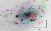 |
Fig. 1. MUSE fields of NGC 300. The red fields are MUSE-GTO data from the Paper I pilot study. The green fields labelled P and Q are additional MUSE-GTO observations for the outer spiral arm. The cyan fields indicate ML20 fields. The magenta fields indicate the previous PN survey area of Peña et al. (2012) using the FORS2 instrument. Image: NGC 300 in Hα taken with the Wide Field Imager (ESO), programme ID 065.N-0076. |
The initial MUSE-GTO data (fields A, B, C, D, E, I, and J) were obtained between the years 2014 and 2016 using the extended wide field mode with a spatial coverage of 1′×1′ and spectral coverage of 4650 − 9350 Å with 1.25 Å sampling. First results from the seven fields in the centre area were reported in Paper I, covering the nucleus, part of the spiral arm that extends from the nucleus to the north-west, and inter-arm regions of the galaxy. In late 2018, additional fields P and Q were observed to cover the part of the outer spiral arm. Moreover, fields A, B, and C were re-observed with adaptive optics support to obtain better image quality. In the adaptive optics mode, a notch filter at 5750 − 6100 Å blocks the laser light, but this does not affect the emission lines of interest. Most of the fields were obtained with an exposure time of 6 × 900 s, with the exception of field J (4 × 900 s), field C (8 × 900 s), and field B, D (11 × 900 s).
The nine MUSE-GTO fields were reduced using the MUSE pipeline (Weilbacher et al. 2020) within the MUSE-WISE environment (Vriend 2015), as explained in more detail in Paper III (Micheva et al. 2022). In addition to the field distortion correction produced by the pipeline, the astrometry is also calibrated using the Gaia DR2 catalogue (Gaia Collaboration 2018), providing absolute astrometry within 0 1. Sky subtraction was performed using an offset field outside the galaxy. Since we perform photometry in [O III]λ5007, we measure the seeing quality at this wavelength based on the full width at half maximum (FWHM) of three to four stars for each field. These stars, which are typically giants or supergiants in the disc of NGC 300, have apparent magnitudes of F606W ≳ 21 in the Hubble Space Telescope (HST) ACS magnitude system (Roth et al. 2018). Unlike the situation in more distant systems, such as Fornax cluster ellipticals (Sextl et al. 2021), confusion with globular clusters is not a concern. For the MUSE-GTO data, the image quality ranges from
  to
to  FWHM, as presented in Appendix C.
Another 35 fields, the ML20 data, publicly available at the ESO archive, were originally observed to study stellar feedback in NGC 300 (McLeod et al. 2020, 2021). The data were obtained using the nominal wide field mode, which has the same spatial coverage of 1′×1′, but with a slightly shorter wavelength coverage of 4750 − 9350 Å. The observations were conducted in the period of 2016–2018 without the support of adaptive optics, and each field was observed with an exposure time of 3 × 900 s. These data were reduced using the fully automated MUSE pipeline (Weilbacher et al. 2020) with default parameters, as provided in the ESO archive. The astrometry of the ML20 data only relied on the distortion correction within each field, which limited the absolute positional accuracy of the object catalogue to ∼3″. Moreover, the sky subtraction was performed using a reference region within each field instead of an offset field; this resulted in sky over-subtraction, especially in areas where diffuse gas is prominent. However, since we perform local sky subtraction for flux measurements of individual objects (see Sect. 3), the effect cancels out. Based on our measurements, the seeing quality of the ML20 data in [O III]λ5007 ranges between  FWHM. These [O III]λ5007 seeing measurements are presented in Appendix C.
3. Data analysis
3.1. PN detection and classification
To find PN candidates, we employed the DELF method described by Roth et al. (2021). This is performed by extracting 15 datacube layers around the wavelength of redshifted [O III]λ5007 (the systematic velocity of NGC 300 is vsys = 144 km s−1; Lauberts & Valentijn 1989) and treating each layer as an on-band image; this 18.75 Å range accounts for the different line-of-sight velocities within the galaxy. Then, an intermediate broadband continuum image is constructed from the wavelength range between λ5063 − 5188 Å, which is free from strong absorption line features; this is used as the off-band image. By subtracting the scaled off-band image (see the scaling factor in Eq. (8) of Roth et al. 2021) from the on-band images, we obtain a series of continuum-free differential images. Using the DS9 software (Joye & Mandel 2003), the differential images are visually inspected to find the [O III]λ5007 sources. After experimenting unsuccessfully with DAOPHOT FIND (Stetson 1987) to identify PN candidates – DAOPHOT FIND was unable to cope with the spatially variable emission line background in [O III]λ5007 – we resorted to the datacube layer blinking technique that is described in Roth et al. (2021).
The typical physical size of a PN is of the of order of ∼0.3 pc (Osterbrock & Ferland 2006). If we assume a distance of 1.88 Mpc (Gieren et al. 2005) and a scale of ∼9 pc/″, we expect the PNe in NGC 300 to appear as point sources. After marking the coordinates of the point sources in [O III]λ5007, we apply aperture photometry (Stetson 1987) at each wavelength layer along the datacube for these objects to obtain their spectra. We employ an aperture diameter of 3 spaxels (0 6), an inner sky annulus of 12 spaxels, and an outer sky annulus of 15 spaxels. Although the seeing conditions of the datacubes vary between
  , we extract the spectra using the same parameters. The small aperture of 3 spaxels is chosen to minimise contamination of background gas or nearby H II regions. Then, the line fluxes are extracted using Gaussian fitting with the LMFIT routine in Python (Newville et al. 2016), keeping in mind that the MUSE data have a wavelength sampling of 1.25 Å. Since the MUSE-GTO and the ML20 data have overlapping areas, the classifications were done independently for each dataset. Cross-matching was performed after the PNe were identified.
To classify the sources into PNe, H II regions, and SNRs, we employed the Baldwin-Phillips-Terlevich (BPT) diagram (Baldwin et al. 1981) that is based on the line ratio of [O III]λ5007/Hβ and [S II]λλ6716, 6731/Hα. Besides the application of classifying active galaxies (Kewley et al. 2001, 2006), the BPT diagram has been demonstrated to effectively discriminate the PNe from their mimics (Kniazev et al. 2008; Frew & Parker 2010; Sabin et al. 2013; Roth et al. 2021). As the classification rely on emission line ratios with very similar wavelengths, we can assume that the relative line fluxes have negligible extinction and seeing dependence on wavelength.
The BPT diagrams for the MUSE-GTO and ML20 data are presented in Fig. 2. To separate the SNRs, we adopted the value log [S II]λλ6716, 6731/Hα ≥ −0.5 from Roth et al. (2021). To discriminate PNe from H II regions, we employed the theoretical line by Kewley et al. (2001), which was originally intended to differentiate starburst galaxies. We also consider the line ratio of [S II]λ6731/6716 as a proxy for density, since bright PNe are expected to be denser than both H II regions and SNRs (Osterbrock & Ferland 2006). While the brightest [O III]λ5007 sources have sufficient line fluxes for the BPT diagram classification, fainter sources may lack the weaker emission lines, namely the Hβ line or the [S II]λ6716, 6731 lines. In such cases, we assume lower limits for the line fluxes and classify the sources as PNe if the [O III]λ5007 line is stronger than the Hα line, which may introduce deviation from the separation lines in the diagram. We also found some faint objects that only have the detection of the [O III]λ5007 and the [N II]λ6584 line without Hα detection and are possibly Type I PNe (Frew & Parker 2010). Moreover, we also put remarks for PNe, which are classified solely based on [O III]λ5007 detection. This is the case for a few of our faintest PN candidates. Nevertheless, such cases will not affect the distance determination because the PNLF cutoff is only defined by the brightest PNe.
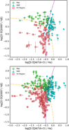 |
Fig. 2. BPT diagram of MUSE-GTO data (upper) and ML20 data (lower). The dot-dashed orange line is taken from Kewley et al. (2001), and the dashed purple line is defined by Roth et al. (2021). Open circles indicate PN candidates, which only have [O III]λ5007 as the diagnostic line for the diagram. The deviation from the separation lines is explained in the text. |
In the MUSE-GTO data, we classified 37 PNe, 62 H II regions, and 59 SNRs. In ML20 data, we classified 85 PNe, 176 H II regions, and 105 SNRs. To cross-match the PN candidates in the overlap area between the two dataset, we attempted an automated algorithm by comparing the sky coordinates. However, since the astrometric accuracy of both data differs, our attempt was not successful. Therefore, the cross-matching was performed visually using the DS9 software (Joye & Mandel 2003). The final PN numbers from the MUSE-GTO and ML20 fields are 105 PNe in the central region and 2 in the P and Q fields at greater galactocentric distances. The PN catalogue is presented in Appendix D.
3.2. PN number comparison
Previous PN surveys of NGC 300 were conducted by Soffner et al. (1996) – SO96, Peña et al. (2012) – PE12, and Roth et al. (2018) – Paper I, who identified 34, 104, and 45 PN candidates, respectively. To demonstrate the accuracy of our classification, we employed the sample by PE12 as comparison, since it covers more area and contains more PNe than the other studies. PE12 observed NGC 300 with the FORS2 imager (Appenzeller et al. 1998) in two 6.8′×6.8′ fields, one in the centre, and another in the eastern outskirts of the galaxy. The study employed the on/off-band technique to detect PN candidates and classified objects based on the criterion of whether or not a central star was present in their 5105 Å image. The expectation was that central stars of PNe would be too faint to be detected in the visual, while the ionising O stars in H II regions could be seen. For brighter candidates with m5007 < 25, they also performed additional spectroscopy using the FORS2 Spectroscopic Mask (MXU) mode (Stasińska et al. 2013). Since our observations cover a smaller area on the sky, we only made the comparison for the intersecting 5′×7′ region in the centre of the galaxy, which is also indicated in Fig. 1.
In the overlapping region at the centre of the galaxy, we identify 105 PNe, compared to 58 in the PE12 sample. Moreover, although we recover all 58 sources found by PE12, our classification indicates several discrepancies. While 43 of the PE12 sources are confirmed as PNe, we classify 9 objects as compact H II regions and 3 as SNRs. These misclassifications could have happened due to the fact that PE12 only have the spectral classification for candidates with m5007 < 25, while the fainter objects completely relied on the detection of a central star. This approach also lacked the ability to identify SNRs amongst the fainter candidates, as such objects can be discriminated through the detection of the [S II]λ6716, 6731 lines (Frew & Parker 2010; Sabin et al. 2013). Since all of our candidates are classified on the basis of their spectral properties, we believe that our classification is more reliable. Moreover, in terms of the number of detection, we also demonstrate that the MUSE observations are more sensitive and able to reach fainter magnitudes.
3.3. [O III]λ5007 photometry
The [O III]λ5007 fluxes were obtained using DAOPHOT aperture photometry (Stetson 1987), applied to the PN candidates in the 15 differential layers for each datacube. Then, the magnitudes were computed using the V-band equivalent conversion (Jacoby 1989) defined as

where the flux is in erg cm−2 s−1. Here, the aperture radius was adjusted to a value of approximately the FWHM of the point spread function (PSF) in a given exposure to accommodate the respective seeing condition. The inner and outer sky annulus were fixed to 12 and 15 spaxels, respectively. Most of the flux of the PSF was obtained by adding the 5 bins closest to the Gaussian peak and the remaining flux is recovered through the use of an aperture correction based on the information of a PSF reference. This correction is crucial for obtaining accurate fluxes but can be a challenge when there is no reference available, especially with the small field of view of MUSE. The aperture correction method is explained in Appendix A.
The photometric uncertainty was calculated from the Gaussian fit errors, convoluted with an assumed flux calibration error of 5% (Weilbacher et al. 2020). In high surface brightness regions of distant galaxies, double-peaked profiles are occasionally found and indicate the presence of two superposed PNe with different radial velocities (Roth et al. 2021). Unsurprisingly, we do not find such cases in our sample. Since NGC 300 is a quite nearby galaxy, spatial coincidences are less likely. Additionally, the five datacube layers containing the total flux for [O III]λ5007 were also inspected to insure the PN candidate was not extended or contaminated by surrounding gas emission.
As an internal test of our photometry, we used the regions of field overlap to compare our PN measurements made in the MUSE-GTO fields to those from the ML20 data. This comparison is presented in the upper panels of Fig. 3. We find that the ML20 observations obtained under poor seeing condition tend to be systematically fainter than the MUSE-GTO data, while the photometry of the same object from different datacubes with similar image quality gives identical results (exception for the faintest PN in the comparison). Thus, the difference in seeing conditions can introduce a magnitude error; this is most likely due to the choice of a too small aperture for the asymptotic assumption for the aperture correction. Because the disc of NGC 300 contains a large amount of diffuse emission-line gas, we chose to not to increase this radius. However, in order to obtain the same photometric quality between the two datasets, we applied and additional corrections of 0.2 mag for objects with seeing  (∼6 spaxels), and 0.3 mag for seeing
  (∼7 spaxels). We found these values based on empirical trial and error to achieve the minimum average discrepancy between the two sets of magnitudes.
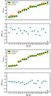 |
Fig. 3. Comparison between the MUSE-GTO and ML20 [O III]λ5007 magnitudes before (upper) and after (lower) photometric correction for PNe in the overlapping area. The markers are linearly scaled with the seeing FWHM of the field and sorted from the brightest to the faintest. |
The comparison after applying the correction is presented in the lower panels of Fig. 3. The average discrepancy is now 0.05 mag, which is still within the typical measurement error of 0.06 mag. For PNe with m5007 ∼ 27 or fainter, the correction has no meaningful implication, because the candidates are close to the detection limit. In the pilot study, Roth et al. (2018) performed a completeness simulation for the MUSE-GTO data of given exposure time, with seeing quality ranging from  . This was conducted by embedding artificial PNe with different magnitudes into the real datacubes. It was found that for a seeing of
  , the expected completeness is 90% at m5007 = 27. Although we are able to detect a PN as faint as m5007 = 28.91, the seeing quality on average for all our data is
  , with 23% of the fields exhibiting larger than
  FWHM. This shows that completeness of 90% at m5007 = 27 is only achieved for 77% of our fields. However, since the emphasis of this work is on the bright candidates that define the PNLF cutoff for the distance determination, our results are not suffering from sample incompleteness at the faint end. For the final [O III]λ5007 magnitudes, we preferred the MUSE-GTO data, if available, and otherwise we employed the ML20 data. We also applied the correction for fields outside the overlapping area with seeing
  . In total, 11 PNe from four fields were corrected in this manner.
To test the accuracy of our photometry, we compared our magnitudes to the results from the literature. Figure 4 shows a comparison with SO96 and PE12. While our data are in reasonable agreement with SO96 within 0.01 mag on average, there is a systematic offset with regard to PE12. We find that our magnitudes are systematically brighter by an average of 0.71 mag. PE12 obtained instrumental [O III]λ5007 magnitudes for the FORS2 on-band image using aperture photometry with the aperture diameter of 5 pixels (1 25), based on the average PSF FWHM of 2.9 pixels. To obtain the apparent m5007 magnitudes, they calibrated the instrumental measurements using an empirical relation derived from the objects’ spectroscopic fluxes, which are only available for the brightest PNe in their sample. We can try to understand what may be the reason for the discrepancy. First of all, we note that flux calibration is an established MUSE procedure in operation at the VLT and part of the data reduction pipeline. According to Weilbacher et al. (2020), flux calibration has been measured to be accurate to within 3–5%. If a significant number of our MUSE exposures were affected by non-photometric observing conditions – for which we have no evidence – we would expect a scattered, but not the tightly constrained, linear correlation, which we see in Fig. 4, in particular for the three brightest magnitudes. Secondly, Roth et al. (2018) have tested synthetic MUSE datacube broadband photometry of stars against published HST photometry for the same GTO datacube subset that has been used in our work, showing no hint of an offset to within a magnitude of F606W = 22.7. Thirdly, the agreement with SO96, who obtained their data with narrow-band imaging at the ESO New Technology Telescope (NTT; i.e. a different instrument at a different telescope), gives us reasonable confidence that our flux calibration cannot be off by as much as a factor of almost 2. Finally, we can follow the argument put forward by Roth et al. (2004), that, by definition, integral field spectroscopy is an ideal tool for spectrophotometry as is does not suffer from any kind of slit effects.
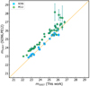 |
Fig. 4. Comparison of m5007 between this work, SO96, and PE12. The photometry of SO96 agrees within 0.01 mag. The photometry of PE12 is systematically fainter by 0.71 mag. For m5007 > 25, the relation with PE12 becomes scattered. |
We can speculate, though, that the spectrophotometry from PE12 might have been affected in various ways to give rise to the observed systematic offset. In case of PE12, the calibration relies on spectroscopic fluxes, which were obtained using a slit spectrograph, and thus may suffered from slit losses that were estimated to be 10 − 15%. However, from our comparison, we infer that the loss might be underestimated since 0.71 mag difference is equivalent to a loss of ∼48%. To test this, we performed a slit-loss simulation based on a model of the PSF with the quoted seeing conditions of  , and a slit size of 1″. The simulation is done in the R band, as the seeing measurement is typically done in this band. Based on these parameters, our simulation predicts that the slit losses should be between 8 − 20%. However, since the PSF FWHM is expected to be larger in the blue wavelength region, the slit loss in [O III]λ5007 will be larger than that in the R band. Moreover, additional losses can be introduced by positioning and guiding errors, as investigated by Jacoby & Kaler (1993). Spectrophotometry with a slit spectrograph also requires the slit to be oriented at the parallactic angle to minimise the effect of atmospheric dispersion (Filippenko 1982; Jacoby & Kaler 1993). Since our observations are performed with an integrated field unit (IFU), we are not affected by any of these problems. While it is possible that our use of small apertures has caused some flux to be lost, we are able to compensate for this loss using aperture corrections as described above. Such a procedure is not easily performed for data observed with a slit spectrograph.
Besides the issue of slit losses, the follow-up spectroscopy by PE12 is limited to PNe with m5007 < 25, which is less than 40% of their whole sample. This implies that most of their PNe are dependant on the measurement accuracy of the brighter PNe, which are likely to be affected by systematic errors. Moreover, the use a 5 pixel aperture to measure the flux for a 2.9 pixel FWHM PSF incurs a risk of including light from background contamination. In such crowded fields with a variable background and ubiquitous diffuse emission-line gas, the aperture might unexpectedly collect [O III]λ5007 flux of the ambient interstellar medium. Without proper background inspection and subtraction, this might lead to an overestimation of brightness. The inclusion of background emission likely explains the scatter for m5007 > 25 in Fig. 4. The spatial resolution of MUSE allows us to carefully check and analyse the condition of the background on a case-by-case basis and provide more accurate photometry. The variable background is also the main consideration to opt for a smaller aperture size for our flux measurements, and to rely on the aperture correction to deliver the final values.
3.4. Balmer decrement
Measurements of extinction using the Balmer decrement with the Hα/Hβ ratio have been demonstrated on MUSE data for different objects: the Pillars of Creation in M16 (McLeod et al. 2015), the core of R136 in the LMC (Castro et al. 2018), and faint H II regions in NGC 300 (Micheva et al. 2022). To obtain this, we employed the spectra extracted for the classification, as explained in Sect. 3.1, using the aperture of 3 spaxels, with the inner and outer sky annulus of 12 and 15 spaxels, respectively. We also apply aperture correction for the Balmer lines (see Appendix A).
However, not all of our PN candidates are detected at these two wavelengths. In order to filter out the candidates, we put a threshold of F(Hα) = 2 × 10⁻¹⁷ erg cm−2 s−1. For typical PNe with electron temperature Te = 10.000 K, the expected Balmer ratio is Hα/Hβ = 2.86 (Osterbrock & Ferland 2006), which corresponds to F(Hβ)∼8.75 × 10⁻¹⁸ erg cm−2 s−1 for the Hα threshold. Any Hβ flux lower than the threshold is too close to the detection limit. For such cases, we assume the upper limit of Hβ flux derived from the Hα line, which consequently also assumes no extinction. To avoid a possible biased exclusion of high-extinction PNe, we flagged the objects with upper limit Hβ flux. If the Hα flux is below the threshold, then the extinction measurement is not performed. Based on the Hα threshold criterion, we have a complete sample for PNe down to m5007 = 24.5. If we extend the sample to fainter magnitudes, we reach 87% completeness until m5007 = 26.0 and 64% completeness until m5007 = 27.0. To calculate the extinction, we then used the Balmer decrement defined as
![$$ \begin{aligned} A_\lambda = k(\lambda ) \, c(\mathrm{H} \beta ) = \frac{ k(\lambda ) \, 2.5}{k(\mathrm{H} \beta )-k(\mathrm{H} \alpha )}\left [\mathrm{log} \, \left ( \frac{\mathrm{H} \alpha }{\mathrm{H} \beta }\right ) - \mathrm{log} \,(2.86) \right ] ,\end{aligned} $$](/articles/aa/full_html/2023/03/aa44597-22/aa44597-22-eq20.gif)
where k(λ) is the wavelength-dependant extinction constant. For the foreground extinction, we employed the extinction curve of Cardelli et al. (1989) with RV = 3.1 and E(B − V) = 0.011 (Schlafly & Finkbeiner 2011). For NGC 300, Bresolin et al. (2009) measured a present-day metallicity of 12 + log(O/H) ∼ 8.1 − 8.5 using the H II regions. A recent measurement using the same MUSE-GTO data based on faint H II regions and diffuse interstellar gas (DIG) also agrees with the latter value as 12 + log(O/H) ∼ 8.5 (Micheva et al. 2022). Since the chemical abundance of NGC 300 in the observation area are similar to the LMC, with 12 + log(O/H) ∼ 8.4 − 8.5 (Toribio San Cipriano et al. 2017), we employed the average LMC extinction curve to obtain the extinction of our PNe. The uncertainty of our extinction measurement is highly dependent on the aperture correction method. Therefore, we quote an estimated error based on the comparison of extinction calculated from different aperture correction methods, as explained in Appendix B.
In spiral galaxies, Herrmann & Ciardullo (2009) found that the typical extinction for the PNe in [O III]λ5007 is A5007 ∼ 0.7. However, we discovered three high-extinction cases with A5007 > 1.5, including one with an extreme value of A5007 ∼ 3.3. While it is possible that some PNe exhibit high intrinsic extinction, as high metallicity populations and massive progenitors tend to produce dustier PNe (Stanghellini et al. 2012), we suspect that the Balmer decrement might not always be accurate due to the local contamination. To investigate this further, and to highlight possible pitfalls that may play a role in studies based on slit spectroscopy, we examined spatial maps of the high-extinction objects in the wavelengths of Hβ, [O III]λ5007, and Hα, using the p3d software (Sandin et al. 2010). We found that these PN candidates are co-spatial with nearby H II regions. In Fig. 5, a PN is shown to be an isolated point source in [O III]λ5007. However, in the spatial map of Hα, the point source is entirely embedded inside the extended emission surface brightness distribution of an unrelated nebula. This clearly shows that the Balmer line flux of the PN candidate is contaminated, and an accurate extinction measurement of the PN itself cannot be obtained. All three of the objects in question show similar patterns of contamination. We therefore excluded them from the sample.
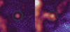 |
Fig. 5. False-colour spatial map in [O III]λ5007 (left) and Hα (right). The flux scaling is identical and logarithmic. The images are 20″ × 20″ (∼180 × 180 pc) each. The green markers illustrate the main and sky aperture. The candidate is isolated in [O III]λ5007 but overlapped with the nearby H II region in Hα. |
We compared our PN extinction measurements with the results from Stasińska et al. (2013) – also referred as ST13 – who observed PNe in NGC 300 with the FORS2-MXU instrument at the VLT (Appenzeller et al. 1998). They used 3 grisms 600B, 600RI, and 300T to cover spectral ranges of 3600 − 5100 Å, 5000 − 7500 Å, and 6500 − 9500 Å, respectively. To avoid uncertainties from the flux calibration of different bands, they employed the Hγ and Hβ lines from the 600B grism spectra to measure the Balmer decrement. The extinction values for 18 PNe in common are presented in Table 1.
Extinction comparison between this work and ST13.
We have contemplated several reasons to explain the discrepancy. Firstly, slit losses that occur for the measurement of [O III]λ5007 most likely also occur for the Hγ and Hβ lines. The short baseline between the lines is also very sensitive to systematic errors, making it difficult to derive accurate extinction values. Moreover, higher order Balmer lines are typically weak. The accuracy of measuring their flux depends on the precision to which the background of stellar absorption line spectra can be subtracted (Jacoby & Kaler 1993; Roth et al. 2004). Using the Potsdam Multi-Aperture Spectrophotometer (PMAS) instrument, Roth et al. (2004) compared the accuracy of the Hβ line flux obtained with the IFU and simulated slits. They demonstrated that the orientation of the slit can introduce a different sampling of the background, leading to systematic differences of the derived flux measurements. Since ST13 performed their measurements with slit spectroscopy, they were susceptible to this type of error.
For cases where the internal extinction of ST13 is reported higher than our values, we find that three of their PNe are discarded from our sample (L6-5, H1-1, and H12-1 in Table 1), either because of severe contamination, as shown in Fig. 5, or by their low excitation, which we consider typical for compact H II regions (Frew & Parker 2010). We also found that in some of these cases, the PN is embedded in diffuse gas. In our sample, if the diffuse gas is assumed to be uniformly distributed, the flux excess can be corrected using the background sky annulus. It remains an open question whether the background correction of diffuse gas was accurately accounted for in the slit spectroscopy of ST13, but we conclude that a careful consideration of background subtraction is critical for the extinction measurements based on the Balmer decrement.
4. The PNLF
The PN luminosity function of this work is presented in Fig. 6. It exhibits the dip between one and three magnitudes below the cutoff. Such a dip is typically observed in star-forming galaxies (Jacoby & De Marco 2002; Ciardullo 2010; Reid & Parker 2010a), which is possibly caused by multiple episodes of star formation (Rodríguez-González et al. 2015; Bhattacharya et al. 2021) or difference in opacity and mass range of the PN formation (Valenzuela et al. 2019).
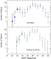 |
Fig. 6. PNLF of NGC 300 using MUSE (top) and PE12 photometry (bottom). The completeness limit for distance measurements is assumed at m5007 = 23.6 and m5007 = 24.0 for ours and PE12, respectively. Open symbols indicate incompleteness. The PNLF dip is visible for both. |
To determine the distance, we employed the maximum likelihood technique, where the empirical PNLF is treated as a probability function (Ciardullo et al. 1989), assuming M* = −4.53 ± 0.06 and a fixed slope parameter of 0.307. When the number of PNe at the bright-end cutoff is less than ∼50, distance determinations based on χ2 minimisation depend significantly on the details of how the PNLF is binned. Such methods are not recommended (Ciardullo et al. 1989; Roth et al. 2021). Although our observation extends to m5007 ∼ 29, the PNLF fit is only performed for the sample brighter than the dip until m5007 = 23.6, since Eq. (1) does not consider the dip feature, which nevertheless is insignificant for the distance determination (Spriggs et al. 2021; Ciardullo 2022). By taking the foreground extinction of E(B − V) = 0.011 (Schlafly & Finkbeiner 2011) into account, the most-likely distance modulus is  with the uncertainties representing the statistical error of the fit and the M* uncertainty.
We also calculated the distance using PE12 photometry to make a comparison. Assuming a completeness limit of m5007 = 24.0, our maximum likelihood approach yields  , a value that is significantly larger than our MUSE distance. We argue that this is due to the systematically fainter magnitudes of PE12 photometry, as discussed in Sect. 3.3. It is important to mention that PE12 measured a modulus distance of
  , a value much smaller than our maximum likelihood values, including our distance measurement using the PE12 data. This difference is possibly due to their use of the Levenberg-Marquardt χ2 fitting technique, which is dependant on the binning method to construct the luminosity function. Since the sample size is limited, they employed rather wide magnitude bins of 1.16 mag, which did result in a luminosity function shape that closely resembles the empirical law. However, in the luminosity function of PE12, their first magnitude bin is located at m5007 ∼ 22, despite the fact that their brightest PN has a magnitude of m5007 = 22.99. Thus, when the fit is performed, this systematic shift to brighter magnitudes results in a smaller distance modulus. This demonstrates that the choice of bin size can produce unintended systematical shifts of the luminosity function when the number of PNe in the top ∼0.5 mag of the luminosity function is small. Similarly, PE12’s choice of bin size also smeared out detail in the PNLF’s shape, as they did not report the observation of the PNLF dip. In Fig. 6, we present the PNLF that we plot with the original data from PE12 using higher binning resolution than the original work. In fact, the dip is present in the PE12 data, confirming that it is not an artefact in our measurements.
Finally, PE12 employed a larger extinction correction for the photometry with A5007 = 0.2 compared to our value of A5007 = 0.05. PE12 assumed this as the intermediate value between found by Gieren et al. (2005) with E(B − V) = 0.096 (A5007 = 0.3) and Schlegel et al. (1998) with E(B − V) = 0.013 (A5007 = 0.05). In the case of Gieren et al. (2005), the extinction value is the sum of both the foreground extinction of Schlegel et al. (1998) and internal extinction derived from the Cepheids. For Cepheid distances, the internal extinction correction is necessary since they are originated from Population I stars, which are typically surrounded by galactic dust. However, this is less true for the PNe, so the foreground extinction correction for the PNLF distance is sufficient (Ciardullo 2010). This implies that the extinction correction A5007 = 0.2 by PE12 is overestimated and also contributes to the smaller distance modulus. Therefore, the discrepancy between our calculation of the PE12 data and the original calculation is traced back to the issue of binning a limited sample and also the extinction correction.
5. Discussion
5.1. PNLF distance
To demonstrate the accuracy of our distance measurement, we compare our result with previous distances in the literature derived using the Cepheids and the TRGB, taken from NED3, in Fig. 7. We can see that most of the distances are within the uncertainties of our PNLF result. One aspect that may introduce the discrepancy is the correction of extinction. For instance, the Cepheid distance of Gieren et al. (2005) and the TRGB distance of Rizzi et al. (2006), both part of the Auracaria project, are corrected with foreground and internal extinction of E(B − V) = 0.096. However, Rizzi et al. (2007) argue that the extinction derived from dusty young Cepheids by Gieren et al. (2005) are not representative for the whole galaxy; their result only applies the foreground component of extinction. This shows the importance of having the same zero-point when comparing different distances derived from different methods.
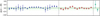 |
Fig. 7. Distance modulus difference between our PNLF result with Cepheids (blue triangles) and TRGB (red squares), obtained from NED and sorted based on publication date. The Cepheid distances are from Willick & Batra (2001), Paturel et al. (2002), Gieren et al. (2004, 2005), Saha et al. (2006), Bono et al. (2010), and Bhardwaj et al. (2016). The TRGB distances are from Butler et al. (2004), Sakai et al. (2004), Tikhonov et al. (2005), Tully et al. (2006), Rizzi et al. (2006, 2007), Jacobs et al. (2009), and Dalcanton et al. (2009). Previous PNLF distances of Soffner et al. (1996) and Peña et al. (2012) are also presented (green circles). The green shadow indicates the uncertainty of our PNLF distance. |
Moreover, we also show that the MUSE observation, combined with the DELF (Roth et al. 2021) and maximum likelihood techniques (Ciardullo et al. 1989), has improved the accuracy of PNLF method, as shown in Fig. 7. The early result by Soffner et al. (1996) is based on the limited sample of only 34 PNe, from which they only construct a cumulative PNLF and employed the distance modulus of the LMC as a yardstick. Peña et al. (2012) identified a significantly larger sample of 104 PNe, but as shown in Sect. 3.3, their data may suffer from slit losses and contamination. The systematically fainter PN magnitudes then led to larger distance modulus, as described in Sect. 4. Since the cutoff of the PNLF of NGC 300 is defined by a very small number of PNe, minimisation fitting methods become too dependant on the binning (Ciardullo et al. 1989). In a study by Jacoby (1997), a correction for PNLF distance based on the number of PN sample is suggested. For a PNLF cutoff sample < 20 PNe, they estimated a distance correction of ∼0.1 mag (see Fig. 5 in Jacoby 1997). However, since the Cepheid and TRGB distance also varies with standard deviation of 0.1 mag, there are no solid distance reference to test if the correction is appropriate. Nevertheless, we have shown that the PNLF distance derived with the maximum likelihood technique is more robust. We take this as a motivation to improve PNLF distance measurements for nearby galaxies with our method.
5.2. Local dust effect on PN extinction
Dust formation plays important role in the early stages of PN evolution since it occurs at the surface of the progenitor asymptotic giant branch (AGB) star and presumably plays an important role in the envelope ejection (Herwig 2005; Stanghellini et al. 2012). Infrared studies in the Milky Way and the LMC have revealed that the dust production is dependant on metallicity, with dustier systems found in higher metallicity environments (Stanghellini et al. 2007, 2012; Bernard-Salas et al. 2009). Although it cannot tell the properties of the dust, Balmer decrement extinction measurements can also probe the presence of dust in PNe. In the study of Davis et al. (2018b), a comparison was made between the PN extinction distribution in the bulge of M31 and several other galaxies: the LMC (Reid & Parker 2010a), NGC 4697 (Méndez et al. 2008b), and NGC 5128 (Walsh et al. 2012). Despite the limited samples involved, the authors found that the average extinction of PNe in each galaxy roughly follows the metallicity of the system.
To investigate such trends in NGC 300, we plot the extinction distribution in [O III]λ5007 for our PNe until m5007 = 23.6 (15 PNe) in Fig. 8. These PNe are the ones employed for the maximum likelihood distance measurement. We find that in general these bright PNe have low extinction in [O III]λ5007. The average extinction value for this sample is A5007 = 0.31 (c(Hβ)∼0.09), which is lower than the average of the bright PNe sample in the LMC with A5007 = 0.57 (Reid & Parker 2010a; Davis et al. 2018b). However, we refrain from further interpreting the extinction distribution with the PN dust production, since the distribution is likely to be affected by local dust clouds, which can vary from one object to another. Such a problem has been reported in NGC 5128, where the high extinction of some PNe was attributed to local dust clouds rather than the PNe themselves (Walsh et al. 2012).
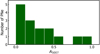 |
Fig. 8. Distribution of extinction measurements for the PNe in [O III]λ5007 until m5007 = 23.6. The average extinction is A5007 = 0.31 (c(Hβ)∼0.09). |
At the distance of NGC 300, our MUSE observations offer a spatial resolution of between 6 and 14 pc. This resolution should be sufficient to visually resolve the spatial variation of dust extinction (Kreckel et al. 2013; Tomičić et al. 2017). To test this, we inspected several objects with high extinction. As an example, we present the spatial map in [O III]λ5007 and red-green-blue (RGB) colours, which is constructed from Johnson-VRI filters, for the PN with the highest extinction value (PN A-23, A5007 = 1.18) in Fig. 9. Although it is not obvious in the [O III]λ5007 image, the RGB image shows a dust lane patch, extending from the lower left corner to the centre. Since PN A-23 is in proximity to the dust lane, we suggest that the measured high extinction of this object is composed of both local dust within the galaxy and circum-nebular extinction associated with the PN itself.
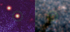 |
Fig. 9. False colour map (left) and RGB colour map (right) of the region surrounding PN A-23. The flux scaling is logarithmic. The images are 20″ × 20″ (∼180 × 180 pc) each. The green markers illustrate the main and sky aperture. The dust patch is clearly visible in the RGB image, overlapped with PN A-23. |
Based on the comparison study between Balmer decrement extinction and infrared dust distribution in M31, Tomičić et al. (2017) concluded that vertical distribution of DIG and dust can vary in different locations of the galaxy and thus cause differing amounts of extinction. For NGC 300, variation of extinction also has been reported by Roussel et al. (2005). Therefore, there is currently no guarantee that the measured extinction of individual PNe is free from local effects, which is confirmed with our images. We must therefore refrain from making conclusions based on the extinction values alone, until the different components of the extinction can be quantitatively resolved.
Although the extinction of individual PNe might be affected by local dust lanes, such effects are less significant for the luminosity function as a whole. The effect of the dust scale height on the PNLF distances of late-type disc galaxies has been discussed by Feldmeier et al. (1997). They modelled PNLF with varying extinction in [O III]λ5007 and concluded that the inferred distance modulus should always be within 0.1 mag of the derived distance without extinction. A similar result also obtained by Rekola et al. (2005), who modelled the PNLF with different scale heights of dust in the starburst galaxy NGC 253. They found that even when the disc was optically thick with 1 mag of extinction, the PNLF distance is robust to within 0.1 mag. Both studies suggest that the brighter PNe tend to be located above the dust layer from the point of view of the observer, or for other reasons suffer little extinction from within the galaxy. With these arguments, we do not expect the occurrence of dust lane extinction to significantly affect our distance result and a correction for internal extinction is at this point not necessary.
5.3. PN parent populations
To gain a better understanding of the parent population of the PNe, we estimate the luminosity and the effective temperature of the central stars of the planetary nebula (CSPNs). These parameters are calculated for PNe until m5007 = 26 with measurable extinction, which corresponds to 87% of the objects within this magnitude limit.
Simulation studies suggest that the maximum conversion efficiency of a central star luminosity into nebular [O III]λ5007 emission is ∼11% (Jacoby 1989; Dopita et al. 1992; Schönberner et al. 2007, 2010; Gesicki et al. 2018). This occurs under the ideal assumption of optically thick nebula and assumes that [O III]λ5007 acts as the sole coolant. If the PN is optically thin, then the efficiency of [O III]λ5007 production is less, and the luminosity inferred for a PN’s central star will be underestimated (Mendez et al. 1992). A high abundance of nitrogen, such as that typically found in Type I PNe (Peimbert & Torres-Peimbert 1983; Phillips 2005), can also increase cooling and lead to an underestimation of central star luminosity. Moreover, the assumption of lower limit extinction for some cases can also underestimate the luminosity. Therefore, we only consider our luminosity estimates as the lower limits.
To estimate the central stars’ effective temperatures, we employed the excitation class method based on the PNe in the LMC (Dopita & Meatheringham 1990; Reid & Parker 2010a). For optically thick PNe, the excitation class temperatures are found to have an empirical correlation with temperature as derived from photo-ionisation modelling (Dopita & Meatheringham 1991; Dopita et al. 1992; Reid & Parker 2010b). To employ this method, we also assume that the metallicity difference between the LMC and NGC 300 is negligible (Bresolin et al. 2009). The revised excitation classes by Reid & Parker (2010b) are defined as
![$$ \begin{aligned}&E_{\mathrm{low} } = 0.45 \left [\frac{F(\lambda 5007)}{F(\mathrm{H} \beta )}\right ] \end{aligned} $$](/articles/aa/full_html/2023/03/aa44597-22/aa44597-22-eq24.gif)
![$$ \begin{aligned}&E_{\mathrm{high} } = 5.54 \left [\frac{F(\lambda 4686)}{F(\mathrm{H} \beta )} \, + \, \mathrm{log} _{10}\frac{F(\lambda 4959) + F(\lambda 5007)}{F(\mathrm{H} \beta )}\right ] , \end{aligned} $$](/articles/aa/full_html/2023/03/aa44597-22/aa44597-22-eq25.gif)
with Elow employed for low-excitation PNe (0 < E < 5) and Ehigh for medium- to high-excitation PNe (5 ≤ E < 12). The empirical relation between the excitation class and effective temperature for optically thick PNe is then defined by Reid & Parker (2010b) as
![$$ \begin{aligned} \mathrm{log} \, T_{\mathrm{eff} } = 4.439 + [0.1174(\mathrm{E} )] - [0.00172(\mathrm{E} ^2)] .\end{aligned} $$](/articles/aa/full_html/2023/03/aa44597-22/aa44597-22-eq26.gif)
Since only the extended mode used in the MUSE-GTO dataset has the wavelength coverage to include the He IIλ4686 line, for uniformity, we determine the excitation class using just the [O III]λ5007 line and Hβ line. This implies that the effective temperatures for medium- and high-excitation PNe with E ≥ 5 (or log Teff ≥ 4.98) are only lower limits. This includes the measurements, which have uncertainties beyond the condition for low-excitation PNe. Based on the six PNe in our sample that have He IIλ4686 detections, we estimate that the effective temperatures can be underestimated by 1.5 − 3 times if we only rely on the Elow. On the other hand, if the nebula is optically thin, based on the study in the LMC, the excitation class temperatures can be overestimated by at least 50% compared to the Zanstra temperatures (Villaver et al. 2007; Reid & Parker 2010b).
Both luminosity and effective temperature estimates rely on the optical thickness of the PNe. To obtain this, we adopt the criterion of [N II]λ6584/Hα ≤ 0.3 as the condition for optically thin PNe (Kaler & Jacoby 1989; Jacoby & Kaler 1989; Reid & Parker 2010b). Since this criterion is not based on nebular modelling in our sample, we use the indication as a more likely condition rather than a definite indicator to explain the possible limitation in our estimations. The estimated stellar parameters are presented in Fig. 10. We include the post-AGB tracks from Miller Bertolami (2016) with a stellar metallicity of Z⊙ = 0.01, which is the closest to the observed value at the central area of NGC 300 with Z⊙ = 0.007 (Kudritzki et al. 2008; Gogarten et al. 2010).
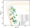 |
Fig. 10. HR diagram of CSPNs in NGC 300. The evolutionary tracks are H-rich post-AGB models by Miller Bertolami (2016). The luminosities are lower limits, assuming a maximum [O III]λ5007 conversion efficiency of 11%. For measurements within the error of log Teff > 4.98, lower limit effective temperatures are assumed. The ratio [N II]λ6584/Hα is the indicator of optical thickness, with a value less of than 0.3 likely indicating optically thinness. Type I PNe are classified with [N II]λ6584/Hα > 1.0. |
A stellar population study by Jang et al. (2020) using the HST found young stars of ∼300 Myr, AGB stars with an age between 1 − 3 Gyr and significant number of RGB stars older than 3 Gyr. From a single stellar evolution perspective, the stellar population of NGC 300 can produce a PN central star mass of ∼0.7 M⊙ from a progenitor mass of 3.0 M⊙, which would have a main sequence lifetime of τMS > 320 Myr (Miller Bertolami 2016). This implies that, theoretically, central stars within any of the stellar tracks in Fig. 10 can be expected. Unfortunately, since most of our luminosities and effective temperatures are lower limits, we are unable to put more constraints on the central star masses at this point.
Within our sample, we also identified several objects as Type I PNe (Peimbert & Torres-Peimbert 1983; Phillips 2005), highly enriched in nitrogen, and classified using [N II]λ6584/Hα > 1. These objects likely arise from younger and more massive stars. For a progenitor mass above ∼2.5 M⊙, the convective envelope in the thermal pulsing AGB phase is likely to extend to the hydrogen-shell burning layer and produce ‘hot bottom burning’ (HBB). This can dredge up the products of the CNO cycle to the surface, to be later expelled by the stellar wind, therefore increasing the nitrogen-to-oxygen ratio in the nebula (Henry et al. 2018). Observations of PNe in M31 by Fang et al. (2018) put a lower limit of ∼2.0 M⊙ for HBB. A more thorough analysis, performed for a Type I PN in the M31 young open cluster B477-D075, yields a HBB lower mass limit of ∼3.4 M⊙ (Davis et al. 2019). This suggests that our approximation for the central star luminosities of Type I PNe is greatly underestimated. For this particular case, we argue that the assumption of [O III]λ5007 as the only coolant is not true. Since the nitrogen-to-oxygen ratio is high, the nitrogen contribution as additional coolant cannot be neglected (Jacoby 1989), causing the underestimation. This might also explain why we did not see the Type I PNe at our PNLF cutoff, although they are expected to have more massive cores than the typical PNe.
More implications regarding the underlying stellar population can also be inferred from the faint end of the PNLF (Ciardullo 2010). However, the current observational study is still limited to a relatively small sample. Recently, based on a very deep survey in M31, Bhattacharya et al. (2021) found that the steep rise in the number of PN fainter M* + 5 mag is caused by the increased mass fraction of a population older than 5 Gyr. For NGC 300, this implies that the photometry should be complete for m5007 > 27. Since our PNLF completeness breaks after m5007 = 27.5, we are unable to provide any insights into this matter at the moment.
5.4. Insights into the most luminous PNe
Numerous simulation studies have been conducted to investigate the nature of the PNe at the cutoff of the luminosity function (Jacoby 1989; Schönberner et al. 2007, 2010; Méndez et al. 2008a; Gesicki et al. 2018; Valenzuela et al. 2019). We review some of them and compare it to our estimated properties to investigate the nature of the most luminous PNe in NGC 300. Using the most recent post-AGB models by Miller Bertolami (2016), simulations of the [O III]λ5007 fluxes for different progenitor mass have been performed by Gesicki et al. (2018). They found that progenitors with the mass range between 1.5 − 3.0 M⊙ are able reach the cutoff absolute magnitude M* = −4.5, assuming that the fluxes at the stellar evolution stages are maximised – also known as maximum nebula hypothesis. It is important to note that the timescale of the 3.0 M⊙ track is too short and less likely to be observed. Additionally, they also performed a simulation with an intermediate nebula hypothesis, where the PNe are predominately opaque; this model suggests that the brightest PNe in the luminosity function will have the luminosity log L/L⊙ = 3.75 ± 0.13. For comparison, the intrinsically most luminous PN in our sample, PN H9-1, has a lower limit luminosity of log L/L⊙ > 3.53. It is also indicated as more likely optically thick, which is in agreement with the simulation. Again, we note that this assumes the ideal 11% maximum efficiency. For example, based on the chemical abundance analysis, the bright PNe in M31 exhibit less conversion efficiency (Jacoby & Ciardullo 1999; Kwitter et al. 2012). Therefore, the actual central star luminosity is likely to be brighter.
Simulation of [O III]λ5007 flux evolution has also been conducted by Schönberner et al. (2007), who employed 1D radiative-hydrodynamical simulations for the nebulae. They calculated that the most luminous PNe that populate the PNLF cutoff will achieve their maximum luminosity at log Teff = 5.00 K and spend ∼500 yr in this phase. For PN H9-1, the lower limit temperature is log Teff > 4.97. They also suggest that UV- to [O III]λ5007 flux conversion process happens most efficiently for central star mass of ∼0.62 M⊙, if the nebular shell remains optically thick during the evolution. Referring to the post-AGB models by Miller Bertolami (2016), the initial mass of the progenitor star would be ∼2.5 M⊙, and the object would spend less than 1000 yr before entering the white dwarf cooling sequence.
Similarly, hydrodynamical models have been used to investigate PNe in nearby galaxies by Schönberner et al. (2010). In these simulations, it was found that central star masses greater than 0.65 M⊙ do not exist at the PNLF cutoff. This also supports the result from Gesicki et al. (2018), in that a progenitor mass of 3.0 M⊙ for PNe is not expected. This also agrees with the progenitor masses between 2.0 − 2.5 M⊙ for the bright PNe in NGC 300 predicted by Stasińska et al. (2013), despite the concerns we mentioned regarding their spectroscopic fluxes in Sect. 3.3. They derived the progenitor masses using the stellar tracks of Bloecker (1995), which evolve more slowly than the recent models of Miller Bertolami (2016). This implies the possibility of less massive progenitors if the new stellar tracks are adopted, which is, however, beyond the scope of our current study.
Recently, the properties of luminous PNe near the PNLF cutoff of M31 have been studied by Davis et al. (2018b) for the bulge, and by Galera-Rosillo et al. (2022) for the disc. For the disc, it was found that the four brightest PNe have an average progenitor mass of 1.5 M⊙, which is lower than the values predicted by Schönberner et al. (2007), but still in agreement with Gesicki et al. (2018). Galera-Rosillo et al. (2022) also measure a relatively low average extinction of the PNe with c(Hβ)∼0.1. This means that the PNe originated from an older stellar population, although the disc of M31 also exhibits star-forming regions.
In contrast, in the older population of the bulge of M31, Davis et al. (2018b) found that the brightest PN have a central star mass > 0.66 M⊙, which means progenitor masses of > 2.5 M⊙. This is found for cases with high extinction, one even reaching c(Hβ)∼0.6, with the average of c(Hβ)∼0.3 for 23 PNe. Current simulations do not predict such massive central stars to be observable, if they exist at all (Schönberner et al. 2010; Gesicki et al. 2018). In old systems, the most luminous PNe are suggested to be products from of blue stragglers – stars that result from a merger during the main sequence (Ciardullo et al. 2005), or symbiotic nebula (Soker 2006). However, both scenarios still do not predict such massive central stars to exist. While the bright Hα background might overestimate the measured extinction, which can lead to the overestimation of luminosity and subsequently the progenitor mass, Davis et al. (2018b) in fact did their measurement with an IFU. Their sky subtraction was based on a PSF model, which was claimed to be accurate within 10%.
Lately, Ueta & Otsuka (2021) suggested that the extinction measurement should be solved iteratively, considering the dependence of Hα/Hβ ratio on the electron temperature (Te) and electron density (ne). Assuming those two parameter as constants would increase the uncertainty of the extinction, and subsequently the stellar parameters. They demonstrate this approach by reanalysing the M31 disc PNe, worked by Galera-Rosillo et al. (2022), and found that the iterative approach yields an average progenitor mass of 2.2 M⊙, instead of 1.5 M⊙ for the four brightest PNe (Ueta & Otsuka 2022). While the extinction does not necessarily affect the Te and ne, it may compromise the ionic and elemental abundance analysis (Ueta & Otsuka 2021, 2022). Since we also assume constant Te and ne for our parameters, we are not excluded from this problem. However, as we are missing the diagnostic lines in the blue spectral region and the ones within MUSE wavelength coverage are below the detection limit, we are unable to put constraints on the Te and ne.
It would be interesting to repeat the exercise of modelling PN spectra on the basis of improved IFU observations that we believe are superior to slit-based spectroscopy in controlling systematic errors, with the more recent stellar evolution tracks and more careful plasma diagnostics. The future BlueMUSE instrument for the VLT (Richard et al. 2019) will offer the capability with a wavelength coverage down to the atmospheric limit in the UV, which includes the necessary nebular lines for such a study.
6. Conclusions
We analysed 44 fields, obtained with the MUSE instrument, to find PNe and construct the PNLF. Using the DELF method (Roth et al. 2021), we identified more than 500 point sources in [O III]λ5007, 107 of which were designated as PNe based on spectral classification with the aid of the BPT diagram (Baldwin et al. 1981). The [O III]λ5007 magnitudes for the PNe were obtained using DAOPHOT aperture photometry (Stetson 1987) with aperture corrections. With the sample completeness at m5007 = 27 for most fields, we constructed the PNLF, which exhibits the dip that has been observed in other star-forming galaxies (Jacoby & De Marco 2002; Ciardullo 2010; Reid & Parker 2010a). To derive the distance, we employed the maximum likelihood estimation method (Ciardullo et al. 1989) to yield a most likely distance modulus  (
( Mpc). For the PNe that are isolated from surrounding emission line sources and exhibit bright enough Balmer lines, we measured their extinction. We estimated parameters of the central stars using the extinction-corrected fluxes in an attempt to track their origin from the underlying stellar population. We discuss the accuracy of our distance measurement, the effect of local dust on our PNe extinction measurements, and the properties of the most luminous PNe in our sample. The conclusions are as follows:
-
The PNLF distance measurement to NGC 300 is improved with our method and is in excellent agreement with Cepheid and TRGB distances. This is due to the spectral information and spatial resolution of MUSE, which provides a higher PN detection per area, better classification, and accurate photometry.
-
With a limited sample, distance determination based on the minimisation technique is highly dependent on the binning. Although coarse binning might provide a better apparent shape of the luminosity function for fitting, it can introduce an unintended systematic shift. Moreover, the details of the PNLF shape, which can provide insights into the stellar population, are also smeared out.
-
The extinction derived for the PNe cannot be completely disentangled from the local dust lane extinction within the galaxy. However, with the spatial resolution of MUSE, we were able to resolve several PNe that are likely obstructed by dust lanes. Any attempt to link the internal extinction and the underlying stellar population requires a quantitative technique to separate the local and internal PN extinction.
-
We find a few Type I PNe that evolved from main sequence mass > 2.5 M⊙. Their luminosities are likely underestimated due to the high abundance of nitrogen that serves as a competing coolant with oxygen. They do not populate our PNLF cutoff.
With these results, and other works reported in the literature, we feel encouraged to further develop the IFU observing technique with MUSE to study extragalactic PNe. One of the inherent parameters that we have not yet utilised is the radial velocity of individual PNe, which is a natural byproduct of the analysis. It will be interesting to find out whether the kinematics can provide hints as to the membership in different populations in NGC 300. Such studies were recently conducted for other disc galaxies: NGC 628 (Aniyan et al. 2018), NGC 6946 (Aniyan et al. 2021), and M31 (Bhattacharya et al. 2019). In the interest of understanding the physical parameters of the PNe, we are currently dependant on the ideal assumption of [O III]λ5007 maximum conversion and excitation classes to derive the central star parameters, which is not ideal, especially when most cases have no He IIλ4686 coverage. Better constraints on the luminosities and effective temperatures are obtainable through nebular abundance modelling. However, the current wavelength coverage of the MUSE instrument hinders the exploration of this possibility. Future IFUs optimised in blue wavelengths, such as BlueMUSE (Richard et al. 2019), will play an important role and allow us to gain more understanding about PNe in the nearby galaxies beyond the Local Group, getting us closer to comprehending the underlying physics behind the constancy of the PNLF cutoff across galaxies.
Acknowledgments
We thank the anonymous referee for a critical reading of the manuscript and helpful suggestions to improve the quality of this paper. Part of this work was supported by the German BMBF program Unternehmen Region, grant 03Z22AN11. PMW gratefully acknowledges support by the BMBF from the ErUM program (project VLT-BlueMUSE, grant 05A20BAB). NC gratefully acknowledges funding from the Deutsche Forschungsgemeinschaft (DFG) – CA 2551/1-1. This research has made use of the NASA/IPAC Extragalactic Database (NED), which is operated by the Jet Propulsion Laboratory, California Institute of Technology, under contract with the National Aeronautics and Space Administration.
References
- Aniyan, S., Freeman, K. C., Arnaboldi, M., et al. 2018, MNRAS, 476, 1909 [Google Scholar]
- Aniyan, S., Ponomareva, A. A., Freeman, K. C., et al. 2021, MNRAS, 500, 3579 [Google Scholar]
- Appenzeller, I., Fricke, K., Fürtig, W., et al. 1998, The Messenger, 94, 1 [NASA ADS] [Google Scholar]
- Bacon, R., Accardo, M., Adjali, L., et al. 2010, SPIE Conf. Ser., 7735, 773508 [Google Scholar]
- Baldwin, J. A., Phillips, M. M., & Terlevich, R. 1981, PASP, 93, 5 [Google Scholar]
- Bernard-Salas, J., Peeters, E., Sloan, G. C., et al. 2009, ApJ, 699, 1541 [NASA ADS] [CrossRef] [Google Scholar]
- Bhardwaj, A., Kanbur, S. M., Macri, L. M., et al. 2016, AJ, 151, 88 [NASA ADS] [CrossRef] [Google Scholar]
- Bhattacharya, S., Arnaboldi, M., Hartke, J., et al. 2019, A&A, 624, A132 [NASA ADS] [CrossRef] [EDP Sciences] [Google Scholar]
- Bhattacharya, S., Arnaboldi, M., Gerhard, O., et al. 2021, A&A, 647, A130 [NASA ADS] [CrossRef] [EDP Sciences] [Google Scholar]
- Bloecker, T. 1995, A&A, 299, 755 [NASA ADS] [Google Scholar]
- Bono, G., Caputo, F., Marconi, M., & Musella, I. 2010, ApJ, 715, 277 [Google Scholar]
- Boyd, J. P. 1978, J. Atmos. Sci., 35, 2236 [NASA ADS] [CrossRef] [Google Scholar]
- Bresolin, F., Gieren, W., Kudritzki, R.-P., et al. 2009, ApJ, 700, 309 [NASA ADS] [CrossRef] [Google Scholar]
- Butler, D. J., Martínez-Delgado, D., & Brandner, W. 2004, AJ, 127, 1472 [NASA ADS] [CrossRef] [Google Scholar]
- Cardelli, J. A., Clayton, G. C., & Mathis, J. S. 1989, ApJ, 345, 245 [Google Scholar]
- Castro, N., Crowther, P. A., Evans, C. J., et al. 2018, A&A, 614, A147 [NASA ADS] [CrossRef] [EDP Sciences] [Google Scholar]
- Ciardullo, R. 2010, PASA, 27, 149 [NASA ADS] [Google Scholar]
- Ciardullo, R. 2012, Ap&SS, 341, 151 [NASA ADS] [CrossRef] [Google Scholar]
- Ciardullo, R. 2022, Front. Astron. Space Sci., 9, 896326 [NASA ADS] [CrossRef] [Google Scholar]
- Ciardullo, R., Jacoby, G. H., Ford, H. C., & Neill, J. D. 1989, ApJ, 339, 53 [Google Scholar]
- Ciardullo, R., Feldmeier, J. J., Jacoby, G. H., et al. 2002, ApJ, 577, 31 [Google Scholar]
- Ciardullo, R., Sigurdsson, S., Feldmeier, J. J., & Jacoby, G. H. 2005, ApJ, 629, 499 [Google Scholar]
- Dalcanton, J. J., Williams, B. F., Seth, A. C., et al. 2009, ApJS, 183, 67 [Google Scholar]
- Davis, B. D., Ciardullo, R., Feldmeier, J. J., & Jacoby, G. H. 2018a, Res. Notes AAS, 2, 32 [NASA ADS] [CrossRef] [Google Scholar]
- Davis, B. D., Ciardullo, R., Jacoby, G. H., Feldmeier, J. J., & Indahl, B. L. 2018b, ApJ, 863, 189 [Google Scholar]
- Davis, B. D., Bond, H. E., Ciardullo, R., & Jacoby, G. H. 2019, ApJ, 884, 115 [NASA ADS] [CrossRef] [Google Scholar]
- Dopita, M. A., & Meatheringham, S. J. 1990, ApJ, 357, 140 [NASA ADS] [CrossRef] [Google Scholar]
- Dopita, M. A., & Meatheringham, S. J. 1991, ApJ, 367, 115 [NASA ADS] [CrossRef] [Google Scholar]
- Dopita, M. A., Jacoby, G. H., & Vassiliadis, E. 1992, ApJ, 389, 27 [Google Scholar]
- Fang, X., García-Benito, R., Guerrero, M. A., et al. 2018, ApJ, 853, 50 [Google Scholar]
- Feldmeier, J. J., Ciardullo, R., & Jacoby, G. H. 1997, ApJ, 479, 231 [NASA ADS] [CrossRef] [Google Scholar]
- Filippenko, A. V. 1982, PASP, 94, 715 [Google Scholar]
- Frew, D. J., & Parker, Q. A. 2010, PASA, 27, 129 [CrossRef] [Google Scholar]
- Fried, D. L. 1966, J. Opt. Soc. Amer. (1917–1983), 56, 1372 [CrossRef] [Google Scholar]
- Fusco, T., Bacon, R., Kamann, S., et al. 2020, A&A, 635, A208 [NASA ADS] [CrossRef] [EDP Sciences] [Google Scholar]
- Gaia Collaboration 2018, VizieR Online Data Catalog: I/345 [Google Scholar]
- Galera-Rosillo, R., Mampaso, A., Corradi, R. L. M., et al. 2022, A&A, 657, A71 [NASA ADS] [CrossRef] [EDP Sciences] [Google Scholar]
- Gerhard, O., Arnaboldi, M., Freeman, K. C., et al. 2005, ApJ, 621, L93 [NASA ADS] [CrossRef] [Google Scholar]
- Gesicki, K., Zijlstra, A. A., & Miller Bertolami, M. M. 2018, Nat. Astron., 2, 580 [NASA ADS] [CrossRef] [Google Scholar]
- Gieren, W., Pietrzyński, G., Walker, A., et al. 2004, AJ, 128, 1167 [NASA ADS] [CrossRef] [Google Scholar]
- Gieren, W., Pietrzyński, G., Soszyński, I., et al. 2005, ApJ, 628, 695 [NASA ADS] [CrossRef] [Google Scholar]
- Gogarten, S. M., Dalcanton, J. J., Williams, B. F., et al. 2010, ApJ, 712, 858 [NASA ADS] [CrossRef] [Google Scholar]
- Henry, R. B. C., Stephenson, B. G., Miller Bertolami, M. M., Kwitter, K. B., & Balick, B. 2018, MNRAS, 473, 241 [NASA ADS] [CrossRef] [Google Scholar]
- Herrmann, K. A., & Ciardullo, R. 2009, ApJ, 703, 894 [NASA ADS] [CrossRef] [Google Scholar]
- Herrmann, K. A., Ciardullo, R., Feldmeier, J. J., & Vinciguerra, M. 2008, ApJ, 683, 630 [Google Scholar]
- Herwig, F. 2005, ARA&A, 43, 435 [NASA ADS] [CrossRef] [Google Scholar]
- Howell, S. B. 1989, PASP, 101, 616 [CrossRef] [Google Scholar]
- Jacobs, B. A., Rizzi, L., Tully, R. B., et al. 2009, AJ, 138, 332 [NASA ADS] [CrossRef] [Google Scholar]
- Jacoby, G. H. 1989, ApJ, 339, 39 [NASA ADS] [CrossRef] [Google Scholar]
- Jacoby, G. H. 1997, in The Extragalactic Distance Scale, eds. M. Livio, M. Donahue, & N. Panagia (Cambridge Cambridge University Press), 197 [Google Scholar]
- Jacoby, G. H., & Ciardullo, R. 1999, ApJ, 515, 169 [CrossRef] [Google Scholar]
- Jacoby, G. H., & De Marco, O. 2002, AJ, 123, 269 [Google Scholar]
- Jacoby, G. H., & Kaler, J. B. 1989, AJ, 98, 1662 [NASA ADS] [CrossRef] [Google Scholar]
- Jacoby, G. H., & Kaler, J. B. 1993, ApJ, 417, 209 [NASA ADS] [CrossRef] [Google Scholar]
- Jacoby, G. H., Ciardullo, R., & Ford, H. C. 1990, ApJ, 356, 332 [NASA ADS] [CrossRef] [Google Scholar]
- Jang, I. S., de Jong, R. S., Minchev, I., et al. 2020, A&A, 640, L19 [NASA ADS] [CrossRef] [EDP Sciences] [Google Scholar]
- Joye, W. A., & Mandel, E. 2003, ASP Conf. Ser., 295, 489 [Google Scholar]
- Kaler, J. B., & Jacoby, G. H. 1989, ApJ, 345, 871 [NASA ADS] [CrossRef] [Google Scholar]
- Kamann, S., Wisotzki, L., & Roth, M. M. 2013, A&A, 549, A71 [NASA ADS] [CrossRef] [EDP Sciences] [Google Scholar]
- Karachentsev, I. D., Grebel, E. K., Sharina, M. E., et al. 2003, A&A, 404, 93 [CrossRef] [EDP Sciences] [Google Scholar]
- Kewley, L. J., Dopita, M. A., Sutherland, R. S., Heisler, C. A., & Trevena, J. 2001, ApJ, 556, 121 [Google Scholar]
- Kewley, L. J., Groves, B., Kauffmann, G., & Heckman, T. 2006, MNRAS, 372, 961 [Google Scholar]
- Kniazev, A. Y., Pustilnik, S. A., & Zucker, D. B. 2008, MNRAS, 384, 1045 [Google Scholar]
- Kreckel, K., Groves, B., Schinnerer, E., et al. 2013, ApJ, 771, 62 [NASA ADS] [CrossRef] [Google Scholar]
- Kreckel, K., Groves, B., Bigiel, F., et al. 2017, ApJ, 834, 174 [NASA ADS] [CrossRef] [Google Scholar]
- Kudritzki, R.-P., Urbaneja, M. A., Bresolin, F., et al. 2008, ApJ, 681, 269 [NASA ADS] [CrossRef] [Google Scholar]
- Kwitter, K. B., Lehman, E. M. M., Balick, B., & Henry, R. B. C. 2012, ApJ, 753, 12 [NASA ADS] [CrossRef] [Google Scholar]
- Lauberts, A., & Valentijn, E. A. 1989, The Surface Photometry Catalogue of the ESO-Uppsala Galaxies (Garching: European Southern Observatory) [Google Scholar]
- Longobardi, A., Arnaboldi, M., Gerhard, O., et al. 2013, A&A, 558, A42 [NASA ADS] [CrossRef] [EDP Sciences] [Google Scholar]
- McLeod, A. F., Dale, J. E., Ginsburg, A., et al. 2015, MNRAS, 450, 1057 [NASA ADS] [CrossRef] [Google Scholar]
- McLeod, A. F., Kruijssen, J. M. D., Weisz, D. R., et al. 2020, ApJ, 891, 25 [NASA ADS] [CrossRef] [Google Scholar]
- McLeod, A. F., Ali, A. A., Chevance, M., et al. 2021, MNRAS, 508, 5425 [NASA ADS] [CrossRef] [Google Scholar]
- Mendez, R. H., & Soffner, T. 1997, A&A, 321, 898 [NASA ADS] [Google Scholar]
- Mendez, R. H., Kudritzki, R. P., & Herrero, A. 1992, A&A, 260, 329 [Google Scholar]
- Méndez, R. H., Teodorescu, A. M., & Kudritzki, R. P. 2008a, ApJS, 175, 522 [CrossRef] [Google Scholar]
- Méndez, R. H., Teodorescu, A. M., Schönberner, D., Jacob, R., & Steffen, M. 2008b, ApJ, 681, 325 [Google Scholar]
- Micheva, G., Roth, M. M., Weilbacher, P. M., et al. 2022, A&A, 668, A74 [NASA ADS] [CrossRef] [EDP Sciences] [Google Scholar]
- Miller Bertolami, M. M. 2016, A&A, 588, A25 [NASA ADS] [CrossRef] [EDP Sciences] [Google Scholar]
- Muñoz-Mateos, J. C., Gil de Paz, A., Boissier, S., et al. 2007, ApJ, 658, 1006 [Google Scholar]
- Newville, M., Stensitzki, T., Allen, D. B., et al. 2016, Astrophysics Source Code Library [record ascl:1606.014] [Google Scholar]
- Osterbrock, D. E., & Ferland, G. J. 2006, Astrophysics of Gaseous Nebulae and Active Galactic Nuclei (Sausalito: University science books) [Google Scholar]
- Paturel, G., Teerikorpi, P., Theureau, G., et al. 2002, A&A, 389, 19 [NASA ADS] [CrossRef] [EDP Sciences] [Google Scholar]
- Peimbert, M., & Torres-Peimbert, S. 1983, IAU Symp., 103, 233 [NASA ADS] [Google Scholar]
- Peña, M., Reyes-Pérez, J., Hernández-Martínez, L., & Pérez-Guillén, M. 2012, A&A, 547, A78 [NASA ADS] [CrossRef] [EDP Sciences] [Google Scholar]
- Peng, C. Y., Ho, L. C., Impey, C. D., & Rix, H.-W. 2002, AJ, 124, 266 [Google Scholar]
- Phillips, J. P. 2005, MNRAS, 361, 283 [NASA ADS] [CrossRef] [Google Scholar]
- Reid, W. A., & Parker, Q. A. 2010a, MNRAS, 405, 1349 [NASA ADS] [Google Scholar]
- Reid, W. A., & Parker, Q. A. 2010b, PASA, 27, 187 [NASA ADS] [CrossRef] [Google Scholar]
- Rekola, R., Richer, M. G., McCall, M. L., et al. 2005, MNRAS, 361, 330 [NASA ADS] [CrossRef] [Google Scholar]
- Richard, J., Bacon, R., Blaizot, J., et al. 2019, ArXiv e-prints [arXiv:1906.01657] [Google Scholar]
- Rizzi, L., Bresolin, F., Kudritzki, R.-P., Gieren, W., & Pietrzyński, G. 2006, ApJ, 638, 766 [NASA ADS] [CrossRef] [Google Scholar]
- Rizzi, L., Tully, R. B., Makarov, D., et al. 2007, ApJ, 661, 815 [Google Scholar]
- Rodríguez-González, A., Hernández-Martínez, L., Esquivel, A., et al. 2015, A&A, 575, A1 [NASA ADS] [CrossRef] [EDP Sciences] [Google Scholar]
- Roth, M. M., Becker, T., Kelz, A., & Schmoll, J. 2004, ApJ, 603, 531 [NASA ADS] [CrossRef] [Google Scholar]
- Roth, M. M., Sandin, C., Kamann, S., et al. 2018, A&A, 618, A3 [NASA ADS] [CrossRef] [EDP Sciences] [Google Scholar]
- Roth, M. M., Jacoby, G. H., Ciardullo, R., et al. 2021, ApJ, 916, 21 [NASA ADS] [CrossRef] [Google Scholar]
- Roussel, H., Gil de Paz, A., Seibert, M., et al. 2005, ApJ, 632, 227 [NASA ADS] [CrossRef] [Google Scholar]
- Sabin, L., Parker, Q. A., Contreras, M. E., et al. 2013, MNRAS, 431, 279 [NASA ADS] [CrossRef] [Google Scholar]
- Saha, A., Thim, F., Tammann, G. A., Reindl, B., & Sandage, A. 2006, ApJS, 165, 108 [Google Scholar]
- Sakai, S., Ferrarese, L., Kennicutt, R. C. Jr., & Saha, A. 2004, ApJ, 608, 42 [NASA ADS] [CrossRef] [Google Scholar]
- Sandin, C., Becker, T., Roth, M. M., et al. 2010, A&A, 515, A35 [NASA ADS] [CrossRef] [EDP Sciences] [Google Scholar]
- Scheuermann, F., Kreckel, K., Anand, G. S., et al. 2022, MNRAS, 511, 6087 [NASA ADS] [CrossRef] [Google Scholar]
- Schlafly, E. F., & Finkbeiner, D. P. 2011, ApJ, 737, 103 [Google Scholar]
- Schlegel, D. J., Finkbeiner, D. P., & Davis, M. 1998, ApJ, 500, 525 [Google Scholar]
- Schönberner, D., Jacob, R., Steffen, M., & Sandin, C. 2007, A&A, 473, 467 [NASA ADS] [CrossRef] [EDP Sciences] [Google Scholar]
- Schönberner, D., Jacob, R., Sandin, C., & Steffen, M. 2010, A&A, 523, A86 [NASA ADS] [CrossRef] [EDP Sciences] [Google Scholar]
- Sextl, E., Kudritzki, R.-P., Weller, J., Urbaneja, M. A., & Weiss, A. 2021, ApJ, 914, 94 [CrossRef] [Google Scholar]
- Soffner, T., Mendez, R. H., Jacoby, G. H., et al. 1996, A&A, 306, 9 [NASA ADS] [Google Scholar]
- Soker, N. 2006, ApJ, 640, 966 [NASA ADS] [CrossRef] [Google Scholar]
- Spriggs, T. W., Sarzi, M., Napiwotzki, R., et al. 2020, A&A, 637, A62 [NASA ADS] [CrossRef] [EDP Sciences] [Google Scholar]
- Spriggs, T. W., Sarzi, M., Galán-de Anta, P. M., et al. 2021, A&A, 653, A167 [NASA ADS] [CrossRef] [EDP Sciences] [Google Scholar]
- Stanghellini, L., García-Lario, P., García-Hernández, D. A., et al. 2007, ApJ, 671, 1669 [NASA ADS] [CrossRef] [Google Scholar]
- Stanghellini, L., García-Hernández, D. A., García-Lario, P., et al. 2012, ApJ, 753, 172 [NASA ADS] [CrossRef] [Google Scholar]
- Stasińska, G., Peña, M., Bresolin, F., & Tsamis, Y. G. 2013, A&A, 552, A12 [NASA ADS] [CrossRef] [EDP Sciences] [Google Scholar]
- Stetson, P. B. 1987, PASP, 99, 191 [Google Scholar]
- Tikhonov, N. A., Galazutdinova, O. A., & Drozdovsky, I. O. 2005, A&A, 431, 127 [NASA ADS] [CrossRef] [EDP Sciences] [Google Scholar]
- Tomičić, N., Kreckel, K., Groves, B., et al. 2017, ApJ, 844, 155 [CrossRef] [Google Scholar]
- Toribio San Cipriano, L., Domínguez-Guzmán, G., Esteban, C., et al. 2017, MNRAS, 467, 3759 [NASA ADS] [CrossRef] [Google Scholar]
- Tully, R. B., Rizzi, L., Dolphin, A. E., et al. 2006, AJ, 132, 729 [NASA ADS] [CrossRef] [Google Scholar]
- Ueta, T., & Otsuka, M. 2021, PASP, 133, 093002 [NASA ADS] [CrossRef] [Google Scholar]
- Ueta, T., & Otsuka, M. 2022, A&A, 667, L8 [NASA ADS] [CrossRef] [EDP Sciences] [Google Scholar]
- Valenzuela, L., Méndez, R., & Miller Bertolami, M. 2019, AAS Meeting Abstracts, 233, 105.01 [NASA ADS] [Google Scholar]
- Villaver, E., Stanghellini, L., & Shaw, R. A. 2007, ApJ, 656, 831 [NASA ADS] [CrossRef] [Google Scholar]
- Vriend, W. J. 2015, Science Operations 2015: Science Data Management– An ESO/ESA Workshop, 1 [Google Scholar]
- Walsh, J. R., Jacoby, G. H., Peletier, R. F., & Walton, N. A. 2012, A&A, 544, A70 [NASA ADS] [CrossRef] [EDP Sciences] [Google Scholar]
- Weilbacher, P. M., Palsa, R., Streicher, O., et al. 2020, A&A, 641, A28 [NASA ADS] [CrossRef] [EDP Sciences] [Google Scholar]
- Willick, J. A., & Batra, P. 2001, ApJ, 548, 564 [NASA ADS] [CrossRef] [Google Scholar]
Appendix A: Aperture correction
The radial profile of a PSF is best modelled with a Moffat function, as a Gaussian often does not accurately match the wings of the PSF (Peng et al. 2002; Kamann et al. 2013). Moreover, flux measurements using a discrete aperture are not able to collect all of the flux from the PSF wings. To recover the lost flux and obtain accurate photometry, we therefore need to apply an aperture correction to our measurements. In order to do this, we need at least one star in a given field as a reference for the observation’s PSF. We examined three to four objects to infer the average PSF FWHM of the frame and chose the best star for the aperture correction. Moreover, we also examined the behaviour of the PSF across wavelengths, as the PSF is expected to be more extended in the blue, and to show a monotonic decrease of the FWHM towards the red (Fried 1966; Boyd 1978; Kamann et al. 2013).
To obtain the aperture correction value, we collected the flux of the reference star using a large aperture radius of 2 4 (or 12 spaxels), assuming that almost all of the flux will be recorded (Howell 1989). Then, by taking the flux of the same star with the aperture size employed for the PNe, we were able to obtain the correction value by taking the ratio of the two fluxes. We then applied this constant to all PNe measurements within the field.
For the Balmer lines, we have to make sure that both lines are corrected in a consistent manner, especially with respect to the wavelength dependence of the PSF. Since the seeing at the telescope is decreasing monotonically with wavelength, the FWHM for Hβ is expected to be larger than the one for Hα, thus changing the aperture correction. The reference stars in each field therefore have to be well behaved across this wavelength range, which was found to not always be the case. We found several apparent point sources that unexpectedly exhibit an increasing PSF FWHM trend to the red. Closer inspection revealed that stellar crowding with luminous red stars, for example, M giants and carbon stars, were responsible for this problem. For Balmer line corrections, we decided to discard the problematic stars as useful PSF references.
As an alternative, we used the brightest PNe that happen to be sufficiently isolated from nearby diffuse gas and H II regions. We then used the PNe’s image profile at the wavelengths of the strong lines of [O III]λ5007 and Hα, while assuming a negligible difference between the PSF at 5007 Åand Hβ. Unfortunately, we found that some of our fields have neither a well behaved star nor bright isolated PNe, so another alternative was needed. Using the best reference stars from different fields and seeing conditions, we derived a simple polynomial relation between the seeing FWHM and the aperture correction value for Hβ, [O III]λ5007, and Hα; these curves are presented in Fig. A.1.
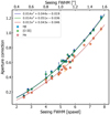 |
Fig. A.1. Empirical polynomial relation between the seeing FWHM and aperture correction for Hβ, [O III]λ5007, and Hα. The relation is derived using 23 stars from different fields. |
We also confirmed that the difference between PSF at Hβ and [O III]λ5007 is not significant, as the polynomial fit is almost identical for the two wavelengths. However, it is important to mention that the relation is only derived using a limited sample of 23 stars. It is not possible to determine the true distribution of this relation and identify the variables that affect it. While this is worthwhile for further investigation, we do not explore it in the current study. We employed the empirical relation as the final alternative, after the bright PN method and the main reference star method. From the 50 PNe that are within the Hα threshold, we corrected 16 PNe with the reference star method, 18 PNe with the bright PN method, and 16 PNe with the empirical relation.
In future studies, the aperture correction can be improved. Firstly, the uncertainties can be minimised under excellent seeing conditions, ideally 0 6 PSF FWHM at the wavelength of [O III]λ5007, which can be achieved using the adaptive optics mode of MUSE. In cases where no field star is available to serve as a PSF reference, modelling the wavelength- and seeing-dependant PSF on the basis of instrumental data from the adaptive optics control software may provide a solution (Fusco et al. 2020).
Appendix B: Extinction uncertainties
The main uncertainty of our extinction measurement is the aperture correction. Since we have only a limited number of objects observed with each correction method, every PN has its own uncertainty, making it difficult to we derive a proper statistical error. As an alternative, we estimate the error based on the comparison of extinction calculated from different aperture correction methods. To perform this, we considered PN candidates that were measured with a well behaved reference star in the field, and a bright PN in the same field. The comparison is presented in Table B.1.
Comparison for extinction values in [O III]λ5007 derived using different aperture correction methods.
Since we expect the aperture correction at Hβ to be larger than the one for Hα, the application of this factor will reduce the inferred extinction, as Hβ appears in the denominator of Eq. (3). In field E, where the initially selected reference star shows the unusual trend of an increasing PSF width to the red, we computed the extinction to be larger after the aperture correction, prompting us to restrict the reference star method only to cases where a well behaved star is available in the field. Moreover, we also see that the use of PNe that are not completely isolated from the ambient gas tends to underestimate the extinction, if compared to other aperture correction methods. Based on our choice of priority of the methods, marked as bold in Table B.1, the difference between the extinction with and without aperture correction (ΔA) is always larger than the difference between extinction values derived using various aperture correction methods. Therefore, we decided to select the ΔA as our error estimates. In cases where the error estimates exceed non-physical negative extinction, the lower limit of the uncertainty is assumed until zero extinction.
We should note, as discussed in Sect. 5.4, that assuming a constant electron temperature Te and ne also introduce uncertainties (Ueta & Otsuka 2021, 2022). Since we did not have the capability to measure Te and ne, we did not include this aspect in our measurement error.
Appendix C: MUSE observation fields
The details of the MUSE fields, both the MUSE-GTO and ML20 (McLeod et al. 2020, 2021), can be referred in Table C.1. We also include the seeing in [O III]λ5007, which obtained based on the average FWHM of 3-4 point sources, preferably stars, in each field.
MUSE observation fields for this work.
Appendix D: MUSE-PN catalogue
The MUSE-PN catalogue of NGC 300 is presented in Table D.1. MUSE-GTO coordinates (accuracy of  ) are presented if available, otherwise ML20 coordinates (accuracy of ∼3″) are provided. The table will be available through the CDS archive and will also include the columns for line fluxes of Hβ, [O III]λ5007, Hα, [N II]λ6584, [S II]λ6716, [S II]λ6731, and the classification remarks.
MUSE-PN catalogue of NGC 300.
All Tables
Comparison for extinction values in [O III]λ5007 derived using different aperture correction methods.
All Figures
|
Fig. 1. MUSE fields of NGC 300. The red fields are MUSE-GTO data from the Paper I pilot study. The green fields labelled P and Q are additional MUSE-GTO observations for the outer spiral arm. The cyan fields indicate ML20 fields. The magenta fields indicate the previous PN survey area of Peña et al. (2012) using the FORS2 instrument. Image: NGC 300 in Hα taken with the Wide Field Imager (ESO), programme ID 065.N-0076. |
| In the text | |
|
Fig. 2. BPT diagram of MUSE-GTO data (upper) and ML20 data (lower). The dot-dashed orange line is taken from Kewley et al. (2001), and the dashed purple line is defined by Roth et al. (2021). Open circles indicate PN candidates, which only have [O III]λ5007 as the diagnostic line for the diagram. The deviation from the separation lines is explained in the text. |
| In the text | |
|
Fig. 3. Comparison between the MUSE-GTO and ML20 [O III]λ5007 magnitudes before (upper) and after (lower) photometric correction for PNe in the overlapping area. The markers are linearly scaled with the seeing FWHM of the field and sorted from the brightest to the faintest. |
| In the text | |
|
Fig. 4. Comparison of m5007 between this work, SO96, and PE12. The photometry of SO96 agrees within 0.01 mag. The photometry of PE12 is systematically fainter by 0.71 mag. For m5007 > 25, the relation with PE12 becomes scattered. |
| In the text | |
|
Fig. 5. False-colour spatial map in [O III]λ5007 (left) and Hα (right). The flux scaling is identical and logarithmic. The images are 20″ × 20″ (∼180 × 180 pc) each. The green markers illustrate the main and sky aperture. The candidate is isolated in [O III]λ5007 but overlapped with the nearby H II region in Hα. |
| In the text | |
|
Fig. 6. PNLF of NGC 300 using MUSE (top) and PE12 photometry (bottom). The completeness limit for distance measurements is assumed at m5007 = 23.6 and m5007 = 24.0 for ours and PE12, respectively. Open symbols indicate incompleteness. The PNLF dip is visible for both. |
| In the text | |
|
Fig. 7. Distance modulus difference between our PNLF result with Cepheids (blue triangles) and TRGB (red squares), obtained from NED and sorted based on publication date. The Cepheid distances are from Willick & Batra (2001), Paturel et al. (2002), Gieren et al. (2004, 2005), Saha et al. (2006), Bono et al. (2010), and Bhardwaj et al. (2016). The TRGB distances are from Butler et al. (2004), Sakai et al. (2004), Tikhonov et al. (2005), Tully et al. (2006), Rizzi et al. (2006, 2007), Jacobs et al. (2009), and Dalcanton et al. (2009). Previous PNLF distances of Soffner et al. (1996) and Peña et al. (2012) are also presented (green circles). The green shadow indicates the uncertainty of our PNLF distance. |
| In the text | |
|
Fig. 8. Distribution of extinction measurements for the PNe in [O III]λ5007 until m5007 = 23.6. The average extinction is A5007 = 0.31 (c(Hβ)∼0.09). |
| In the text | |
|
Fig. 9. False colour map (left) and RGB colour map (right) of the region surrounding PN A-23. The flux scaling is logarithmic. The images are 20″ × 20″ (∼180 × 180 pc) each. The green markers illustrate the main and sky aperture. The dust patch is clearly visible in the RGB image, overlapped with PN A-23. |
| In the text | |
|
Fig. 10. HR diagram of CSPNs in NGC 300. The evolutionary tracks are H-rich post-AGB models by Miller Bertolami (2016). The luminosities are lower limits, assuming a maximum [O III]λ5007 conversion efficiency of 11%. For measurements within the error of log Teff > 4.98, lower limit effective temperatures are assumed. The ratio [N II]λ6584/Hα is the indicator of optical thickness, with a value less of than 0.3 likely indicating optically thinness. Type I PNe are classified with [N II]λ6584/Hα > 1.0. |
| In the text | |
|
Fig. A.1. Empirical polynomial relation between the seeing FWHM and aperture correction for Hβ, [O III]λ5007, and Hα. The relation is derived using 23 stars from different fields. |
| In the text | |
Current usage metrics show cumulative count of Article Views (full-text article views including HTML views, PDF and ePub downloads, according to the available data) and Abstracts Views on Vision4Press platform.
Data correspond to usage on the plateform after 2015. The current usage metrics is available 48-96 hours after online publication and is updated daily on week days.
Initial download of the metrics may take a while.