| Issue |
A&A
Volume 671, March 2023
|
|
|---|---|---|
| Article Number | A17 | |
| Number of page(s) | 17 | |
| Section | Cosmology (including clusters of galaxies) | |
| DOI | https://doi.org/10.1051/0004-6361/202243899 | |
| Published online | 01 March 2023 | |
UNIONS: The impact of systematic errors on weak-lensing peak counts⋆
1
Observatoire de Paris, Université PSL, 61 avenue de l’Observatoire, 75014 Paris, France
e-mail: This email address is being protected from spambots. You need JavaScript enabled to view it.
2
Université Paris-Saclay, Université Paris-Cité, CEA, CNRS, Astrophysique, Instrumentation et Modélisation Paris-Saclay, 91191 Gif-sur-Yvette, France
3
Institut d’Astrophysique de Paris, UMR 7095, CNRS & Sorbonne Université, 98 bis boulevard Arago, 75014 Paris, France
4
Institute for Particle Physics and Astrophysics, Department of Physics, ETH Zürich, Wolfgang Pauli Strasse 27, 8093 Zürich, Switzerland
5
Université de Paris, CNRS, Astroparticule et Cosmologie, 75013 Paris, France
6
Laboratoire d’Astrophysique de Marseille, Aix-Marseille Univ., CNRS, CNES, 13388 Marseille Cedex 13, France
7
Department of Physics and Astronomy, University of Waterloo, Waterloo, ON N2L 3G1, Canada
8
Waterloo Centre for Astrophysics, Waterloo, ON N2L 3G1, Canada
9
Perimeter Institute for Theoretical Physics, 31 Caroline St. N., Waterloo, ON N2L 2Y5, Canada
Received:
29
April
2022
Accepted:
28
October
2022
Abstract
Context. The Ultraviolet Near-Infrared Optical Northern Survey (UNIONS) is an ongoing deep photometric multiband survey of the northern sky. As part of UNIONS, the Canada-France Imaging Survey (CFIS) provides r-band data, which we use to study weak-lensing peak counts for cosmological inference.
Aims. We assess systematic effects for weak-lensing peak counts and their impact on cosmological parameters for the UNIONS survey. In particular, we present results on local calibration, metacalibration shear bias, baryonic feedback, the source galaxy redshift estimate, intrinsic alignment, and cluster member dilution.
Methods. For each uncertainty and systematic effect, we describe our mitigation scheme and the impact on cosmological parameter constraints. We obtain constraints on cosmological parameters from Monte Carlo Markov chains using CFIS data and MassiveNuS N-body simulations as a model for peak counts statistics.
Results. Depending on the calibration (local versus global, and the inclusion or not of the residual multiplicative shear bias), the mean matter density parameter, Ωm, can shift by up to −0.024 (−0.5σ). We also see that including baryonic corrections can shift Ωm by +0.027 (+0.5σ) with respect to the dark-matter-only simulations. Reducing the impact of the intrinsic alignment and cluster member dilution through signal-to-noise cuts leads to larger constraints. Finally, with a mean redshift uncertainty of Δz̄ = 0.03, we see that the shift in Ωm (+0.001, which corresponds to +0.02σ) is not significant.
Conclusions. This paper investigates, for the first time with UNIONS weak-lensing data and peak counts, the impact of systematic effects. The value of Ωm is the most impacted and can shift by up to ∼0.03, which corresponds to 0.5σ depending on the choices for each systematics. We expect constraints to become more reliable with future (larger) data catalogs, for which the current pipeline will provide a starting point. The code used to obtain the results is available on GitHub.
Key words: large-scale structure of Universe / gravitational lensing: weak / methods: data analysis
© The Authors 2023
 Open Access article, published by EDP Sciences, under the terms of the Creative Commons Attribution License (https://creativecommons.org/licenses/by/4.0), which permits unrestricted use, distribution, and reproduction in any medium, provided the original work is properly cited.
This article is published in open access under the Subscribe to Open model. This email address is being protected from spambots. You need JavaScript enabled to view it. to support open access publication.
1. Introduction
Weak gravitational lensing has been used as a cosmological probe in recent years with great success, for example with Dark Energy Survey1(DES), Kilo-Degree Survey2 (KiDS), Hyper Suprime-Cam3 (HSC), and Canada France Hawaii Lensing Survey4 (CFHTLens). It corresponds to the small distortions we observe in the images of background sources (such as high-redshift galaxies) due to the deflection of photons as they pass through tidal fields in the large-scale structure (LSS) in the Universe (Bartelmann & Schneider 2001).
Second-order statistics of weak lensing, such as the two-point correlation function or the power spectrum, only capture the Gaussian part of the LSS (Weinberg et al. 2013). Its non-Gaussian part, which is induced by the nonlinear evolution of structure on small scales and low redshifts, contains, however, a wealth of information about cosmology. Several higher-order statistics, such as Minkowski functionals (Kratochvil et al. 2012; Parroni et al. 2020), higher-order moments (for example, Petri et al. 2016; Gatti et al. 2020), the bispectrum (Takada & Jain 2004; Coulton et al. 2019), peak counts (Kruse & Schneider 1999; Dietrich & Hartlap 2010; Liu et al. 2015b; Lin & Kilbinger 2015; Peel et al. 2017; Martinet et al. 2017; Li et al. 2019; Ajani et al. 2020, and references therein), the starlet ℓ1 norm (Ajani et al. 2021), the scattering transform (Cheng et al. 2020), wavelet phase harmonic statistics (Allys et al. 2020), and machine learning-based methods (Fluri et al. 2018, 2022; Shirasaki et al. 2021, among others), have been introduced to account for non-Gaussian information.
In this work we choose to focus on peak counts extracted from real data, using the pipeline developed to perform the study presented in Ajani et al. (2020), which had previously only been tested on simulations. Peaks in weak-lensing convergence maps are tracers of overdense regions. They are the local maxima defined as a pixel that is larger than all eight of its neighbors. The peak function – that is, the number of peaks as a function of peak height (in a convergence map) or signal-to-noise ratio (S/N) – depends on the nonlinear and non-Gaussian part of the LSS. This higher-order weak-lensing statistic can be used to constrain cosmological parameters. Peak counts are complementary to second-order shear statistics (Jain & Waerbeke 2000), and by combining both parameters degeneracies can be removed (Dietrich & Hartlap 2010).
Weak-lensing peaks are an indirect tracer of dark-matter halos: large peaks are strongly correlated with massive halos, whereas lower-amplitude peaks are generally created by multiple smaller halos along the line of sight (Yang et al. 2011). Low-amplitude peaks can also be caused by mass outside dark-matter halos, or by galaxy shape noise (Liu & Haiman 2016; Yang et al. 2011).
Explicit expressions or complete theoretical predictions of peak counts are still an active area of research. It is, however, possible to generate weak-lensing simulations densely sampled in cosmological parameter space in order to interpolate them and use the interpolation as a prediction. The advantage of simulations is the possibility to incorporate the exact survey mask and shape noise. For example, Dietrich & Hartlap (2010) created a set of N-body simulations in the (Ωm, σ8) plane for 158 cosmologies, and Liu et al. (2015b) and Kacprzak et al. (2016) used ray-tracing N-body simulations in the (Ωm, σ8, w) plane for 91 cosmologies. Here we use the MassiveNuS simulations (Liu et al. 2018) to predict peak counts as in Li et al. (2019) and Ajani et al. (2020). These simulations are described in more detail in Sect. 3.
The first cosmological constraints from peak counts were obtained on real data by Liu et al. (2015a) using the Canada-France-Hawaii Telescope (CFHT) Stripe 82 Survey, and by Liu et al. (2015b), using CFHTLenS data. DES Science Verification data have been analyzed by Kacprzak et al. (2016). KiDS 450 deg2 data have been studied by Shan et al. (2017) and Martinet et al. (2017). The first tomographic analysis was performed by Harnois-Déraps et al. (2021b) for the DES-Y1 data release. Recently, Zürcher et al. (2022) analyzed the DES-Y3 data release using an emulator approach. These analyses all use peak counts and complement second-order statistics analyses, constraining cosmological parameters.
Weak-lensing observables have to be corrected for systematic effects, which can have an observational and astrophysical origin and can induce biases into the cosmological constraints if not properly taken into account. These artifacts can easily be created by the atmosphere, the telescope, and the detector, and during the data analysis. Astrophysical correlations such as intrinsic galaxy alignments add to the lensing correlations in a nontrivial way. Furthermore, to be able to interpret weak-lensing observables in a cosmological context, the physics of small scales needs to be reliably estimated.
Extensive studies of many of these systematics for second-order statistics exist, for example Massey et al. (2012), Troxel & Ishak (2015), Hildebrandt et al. (2016), and Mandelbaum (2018). For current and future surveys, precise requirements on the instrument and data processing are routinely derived for those statistics. However, how to properly include systematic effects in the context of higher-order statistics is an ongoing research topic (Kacprzak et al. 2016; Coulton et al. 2020; Zürcher et al. 2021; Harnois-Déraps et al. 2021a; Pyne & Joachimi 2021).
This paper is the first to study several weak-lensing systematics and uncertainty, their effect on peak counts, and the resulting constraints on cosmological parameters from the Ultraviolet Near-Infrared Optical Northern Survey (UNIONS)/Canada-France Imaging Survey (CFIS) galaxy survey. In addition, we develop a novel method for locally calibrating the measured shear, including shear and selection biases. We investigate mitigation schemes for these effects and quantify biases in cosmological parameters.
This paper is organized as follows: In Sects. 2 and 3 we describe the data and simulations used in this work, respectively. In Sect. 4 we describe the measurement of weak-lensing peak counts. In Sect. 5 we introduce local shear calibration and compare it to the standard global calibration. In Sect. 6 we present results for each of the studied biases and uncertainties and discuss mitigation methods. Finally, we draw our conclusions in Sect. 7.
2. Data
2.1. Image processing
We used weak-lensing data from UNIONS5. This ongoing survey will provide 4800 deg2 of multiband photometric images in the Northern Hemisphere. Founded in 2018, UNIONS is a collaboration of several groups and surveys, each providing data in different bands. These participating surveys are CFIS, the Panoramic Survey Telescope And Rapid Response System (Pan-STARRS), Wide Imaging with Subaru HSC of the Euclid Sky (WISHES), and the Waterloo Hawai’i IfA G-band Survey (WHIGS).
For the CFIS part of the survey r- and u-band images are taken at the CFHT with MegaCAM, a wide-field optical imaging facility. The CFIS r-band images have a median seeing of 0.65 arcsec reflecting the extremely stable atmosphere at Manua Kea together with the excellent CFHT optical system. Each observed sky location is covered by at least three single exposures, which are dithered by one-third of the focal plane, or 0.33°. The exposure time varies between 100 and 300 s, where smaller exposure times are chosen in better observing conditions. This survey strategy provides images of a very homogeneous depth. In this work, we only use r-band data from CFIS for our weak-lensing peak count study. In particular, the weak-lensing data from P3, a patch of size 34.7 × 17.7 deg2 is analyzed. This patch overlaps with CFHTLenS, which is used to infer the redshift distribution (see Sect. 2.3). These data have been processed and validated (see Guinot et al. 2022 for details). The preprocessing of the CFHT data consists of a calibration step with the MegaPipe pipeline (Gwyn 2008). The single exposures are first calibrated before they are combined with SWARP6 to build stacked images. MegaPipe provides an astrometric calibration of the survey using Gaia Data Release 2 (Gaia Collaboration 2018), and photometric calibration of the r-band data relative to the Pan-STARRS1 survey (Chambers et al. 2016). Both astrometric and photometric calibration are excellent so we do not expect calibration errors to significantly impact weak-lensing measurements (Guinot et al. 2022).
2.2. The weak-lensing catalog
Since the stacks have a larger S/N than the single-exposure images, we use the former to detect galaxy candidates. Due to the large dithers, the point-spread function (PSF) on the stacks is very inhomogeneous and discontinuous. For this reason, we detect stars and construct the PSF model on single exposures. Galaxy shapes are then obtained using the multi-epoch model-fitting method ngmix (Sheldon & Huff 2017)7. Those measurements are calibrated with metacalibration (Huff & Mandelbaum 2017) to provide shear estimates. The creation and validation of the shear catalog are fully described in Guinot et al. (2022). We note that this is a preliminary version, called “version 0”, of the catalog where the source density is conservative and does not reflect future versions of the CFIS shear data. Specifics of the shear catalog are presented in Table 1.
P3-CFIS survey specifications.
2.3. Redshift distribution of source galaxies
Multiband data of UNIONS are still sparse, and photometric redshifts have not been obtained yet. Using the r-band data only, redshifts have been obtained for a population of galaxies with two different methods, as follows.
For both methods, CFIS galaxies were matched to the deeper CFHTLenS on the 50 deg2 W3 field. First, Guinot et al. (2022) approximated the CFIS redshift distribution as the histogram of the best-fit photometric redshifts from CFHTLenS of that matched subsample. Photo-z’s for CFHTLenS had been obtained in Hildebrandt et al. (2012) from u, g, i, r, z multiband data, calibrated with various spectroscopic deep data sets. Second, employing the direct calibration technique, Spitzer et al. (in prep.) re-weighted the Deep Extragalactic Evolutionary Probe 2 (DEEP2) spectroscopic sample (Newman et al. 2013) in a 5D space spanned by the u, g, i, r, z photometric bands, to match the density of the matched subsample in that space. The re-weighted DEEP2 spectroscopic redshift distribution is an estimate of the CFIS n(z). This distribution was fit in Spitzer et al. (in prep.) by an analytical function with two components. The first, exponential, component accounts for the bulk of the distribution, whereas the second, Gaussian, term, models the tail at z > 2. However, the addition of this second term somewhat overestimates the re-weighted DEEP2 redshift distribution between z = 1.5 and 2.
The mean redshift is obtained as  , where the integral over the normalized redshift distribution n(z) is carried out nominally up to the limiting redshift of the survey, zmax. Both redshift distributions have a significantly non-vanishing probability at high redshifts z ≳ 2. This is most likely not a physical feature, since we do not expect a large number of galaxies in the CFIS sample at those redshifts.
Our best estimate of  is obtained by integrating over the CFHTLenS-matched n(z) with a limit of zmax = 2, resulting in
  . Table 2 presents alternative estimates with varying n(z) and zmax. Three further, reasonable combinations yield a slightly higher
  of 0.68. We use this alternative value in Sect. 6.3 to test the impact of the estimated redshift uncertainty.
Mean redshift,  , of CFIS weak-lensing galaxies for different redshift distributions, n(z), and maximum redshifts, zmax.
3. Simulations
To get the predictions for the summary statistics that we use to perform cosmological inference, we employed the MassiveNuS simulations, a suite of cosmological dark-matter-only N-body simulations that explore different cosmologies including massive neutrinos in the range ∑mν = 0 − 0.62 eV. The simulations have a 512 Mpc h−1 box size with 10243 cold dark matter particles. The pixel size is 0.4 arcmin. The implementation is performed using a modified version of the public tree-Particle Mesh (tree-PM) code Gadget28 with a neutrino patch, describing the effect of massive neutrinos on the growth of structures up to k = 10h Mpc−1. A complete description of the implementation and the products is provided in Liu et al. (2018). The cosmological parameters vary across the simulations within the range Mν ∈ [0, 0.62], Ωm ∈ [0.18, 0.42], and As ∈ [1.29, 2.91]×10−9. We thus worked on the constraints on these three cosmological parameters, which are well sampled by the simulations. They include the effects of radiation on the background expansion and the impact of massive neutrinos is included with a linear-responds method: neutrinos are evolved perturbatively, while their clustering is caused by the nonlinear dark-matter evolution.
The simulations assume a flat universe with Hubble constant H0 = 70 km s−1 Mpc−1. The primordial power-spectrum scalar index is ns = 0.97, the baryon density Ωb = 0.046, and the dark-energy equation of state w = −1. A fiducial cosmology is set to [Mν, Ωm, 109 × As]=[0.1, 0.3, 2.1]. Simulations are available for 101 cosmologies, with 10 000 realizations for each cosmology, obtained by randomly rotating and shifting the lensing potential planes.
Following Ajani et al. (2020), the peak counts were computed for each of the MassiveNuS cosmologies from the simulated convergence maps, averaged over the 10 000 realizations for each model. A model with massless neutrinos corresponding to [Mν, Ωm, 109 × As]=[0.0, 0.3, 2.1] is also provided, and we used it to compute the covariance matrix.
3.1. Effective redshift distribution
For each of the 101 cosmological models, five source redshifts, zs = {0.5,1.0,1.5,2.0,2.5}, are present. To match the simulations to the observed redshift distribution of CFIS, we made the following approximations. We matched the mean redshift between MassiveNuS and CFIS (Sect. 2.3) and neglected the shape of the redshift distribution. For that, we interpolated the two convergence maps closest in redshift to  and obtained the new effective map as
 (1)
(1)
This effectively defines the new redshift distribution by a weighted sum of two Dirac delta distributions,
 (2)
(2)
To match our best estimate,  , we set λ = 0.7. As anticipated in Sect. 2.3, we also employed
  in order to estimate the uncertainty related to the redshift estimation. To do so, we used the relation in Eq. (1) to the new effective maps at
  and κz = 1 and imposed
  . This results in an interpolation parameter λ′ = 0.91.
3.2. Noise
To include the CFIS shape noise in the simulations that we employ to perform inference, we add Gaussian noise. First, we compute the global ellipticity dispersion  . The ellipticity noise per smoothed pixel is then
 (3)
(3)
where ngal is the galaxy number density and Apix is the pixel size. For CFIS data, we used the value listed in Table 1. We applied the Gaussian noise to the convergence maps because we do not have direct access to the simulated shear.
4. Weak-lensing peak counts
We employed weak-lensing peak counts as summary statistics for our analysis, measured from the weak-lensing convergence maps.
4.1. Convergence maps
The reduced shear g is the main observable in weak gravitational lensing by galaxies, it is estimated from galaxy ellipticities. We can define it as
 (4)
(4)
where γ is the shear and κ the convergence. For the data, the E- and B-mode convergence maps are built through Kaiser-Squires inversion (Kaiser & Squires 1993) from the reduced shear provided by the weak-lensing catalog. The CFIS-P3 map is quite large for a projection but peaks are local, and any distortion will rather affect large scales. In our analysis we worked with the E-mode of the convergence map as the B-mode contain mostly noise (Guinot et al. 2022). Hereafter, when we speak about convergence, we mean the E-mode of the convergence map. The CFIS-P3 convergence map is shown in Fig. 1. Every pixel has a size of 0.4 arcmin, as in the simulations. The 13 black squares are boxes of 512 × 512 pixels, which correspond to the size of the simulation convergence maps. These boxes are placed such that they do not overlap with larger masked or missing areas.
 |
Fig. 1. Convergence map of the CFIS-P3 patch. The squares indicate the regions free of large masks, which were used to compute the peak count. The total peak count is the mean of the peaks over the 13 patches. |
For the simulations, we employed the already existing maps from the MassiveNus9 suite, obtained with the LensTools10 (Petri 2016) ray-tracing package. We mimicked the CFIS shape noise by adding the noise introduced in Sect. 3.2 to the maps coming from the simulations, and we smoothed them with a Gaussian kernel of width σ = 2 arcmin. Li et al. (2019) find that for the same simulations, using peak counts, the optimal smoothing to get tighter constraints is 2 arcmin. As a first work, we chose this smoothing scale to be consistent with the simulations. Moreover, Hildebrandt et al. (2016) find that a smoothing scale of 2 arcmin is a good choice for KiDS data, which have the same number of galaxies per pixel as us. For future work, it can be interesting to adapt simulations to the data to determine the optimal smoothing scale for future releases. We thus computed signal-to-noise ratio (S/N) maps, where the S/N is defined as the noisy convergence map, smoothed with a Gaussian filter over the standard deviation of the noise defined in Eq. (3). Then we computed the peak counts with the lenspack11 python package on the S/N maps collecting the local maxima, namely computing the pixels with higher values with respect to their neighboring pixels. In our analysis, we consider linearly spaced bins in the range S/N = [ − 2, 6]. The peak counts distribution used for parameter inference (Sect. 6) corresponds to the mean of the peak counts from the 13 patches. This corresponds to an area of 13 × 12.25 deg2 ≈ 160 deg2. Figure 2 presents the S/N map and the peak counts histogram from one patch of the CFIS-P3 data.
 |
Fig. 2. S/N map and peak counts histogram. The left plot is the S/N map of a part of the 512 × 512 pixels of CFIS-UNIONS data. The right plot is the peak counts computed on that S/N map. |
4.2. Modeling and parameter inference
We modeled the peak function with the MassiveNuSN-body and ray-tracing simulations (Liu et al. 2018). In these simulations the matter density parameter, Ωm, the primordial power-spectrum normalization amplitude, As, and the total mass of neutrinos, Mν = ∑mν, were varied (see Sect. 3 for more details). We constructed a likelihood function as follows. First, the theoretical model was obtained by numerically computing the peak function for each simulated parameter combination. These functions were then interpolated to arbitrary parameters within the parameter boundaries using a Gaussian process. The error of prediction was always below the CFIS statistical error and on the order of a few per cent. The covariance matrix was computed from the variations of realizations at the fiducial model and is thus assumed to be parameter-independent. As explained in the previous section, for the data, the peaks were computed as the mean of the peaks on 13 mask-free patches; thus, the re-scaling factor of the covariance when we infer parameters from the data is 1/13. The likelihood was taken as a multivariate Gaussian as a function of the data vector. As prior on the parameters, we used a flat prior for the three parameters: Mν ∈ [0.06, 0.62], Ωm ∈ [0.18, 0.42] and As ∈ [1.29, 2.91]×109. The prior of Ωm and As are the bounds of the simulation. For Mν, 0.06 is the minimum from oscillation experiments (Particle Data Group 2016) and 0.62 is the upper bound of the simulations. We explored the posterior distribution with Monte Carlo Markov chain (MCMC) sampling using the python package emcee. Specifically, we employed 250 walkers initialized in a tiny Gaussian ball of radius 10−3 around the fiducial cosmology [Mν, Ωm, 109 × As]=[0.1, 0.3, 2.1] and estimated the posteriors using 6500 sampling steps and 200 burn-in steps.
5. Local shear calibration
In this section, we describe and measure a spatially varying calibration of the estimated shear. For the multiplicative shear bias, including both shear and selection biases, we use the technique of “metacalibration” (Huff & Mandelbaum 2017), which we briefly describe in the following subsection.
5.1. Metacalibration
This method consists in measuring the response matrix R of a shape measurement algorithm to a shear artificially applied to an image. The ith component of the observed ellipticity of a galaxy, εi, is an estimator of the galaxy shear,  , however, not an unbiased estimator in general. The linearized relation between true and estimated shear for a given galaxy can be written as
 (5)
(5)
where the response matrix can be described as  and ci is the additive bias. The trace of the shear response matrix is also parameterized as tr (R) = 2(1 + m) where m is the multiplicative shear bias.
We numerically compute the shear response matrix by replacing the derivative with finite differences. For this, we create four new images for each detected galaxy. These images are deconvolved with the model PSF at that position, then sheared in two directions for both shear components, and re-convolved with a circularized PSF that is slightly larger than the original one. We note that a fifth image is created, which is unsheared but has the same re-convolved PSF. This image is used to measure shapes that are consistent with the metacalibration correction.
The response matrix has two additive components, the shear response matrix and the selection response matrix, both of which can be computed via metacalibration, as follows. First, the shear response matrix is computed for each galaxy individually. Denoting with  the observed shear of the galaxy image sheared by ±Δg in the j direction, we get
 (6)
(6)
We used Δg = 0.01. Since this is a very noisy measurement, often resulting in singular matrices, we compute the mean value over all galaxies,
 (7)
(7)
Second, the selection response matrix quantifies selection biases originating from correlations between shear and selection-dependent image properties. For example, if a cut is applied on the S/N of the galaxy sample and the S/N varies with shear, the effective sample shear after the cut is modified, and no longer representative of the underlying population shear, which introduces a bias.
The selection matrix cannot be obtained for a single galaxy, but only for a sample of galaxies. For that, we first apply our selection S to the four samples of sheared galaxies. This provides us with a selection mask S±, j for each of the four cases. These four masks are now in turn applied to the fifth sample without added shear. We compute the mean observed shear for each of the four masked samples, denoted as  . Any difference in these mean values is due to shear-dependent selection criteria, and can be used to define the selection response matrix as
 (8)
(8)
The total mean response matrix is
 (9)
(9)
The estimated shears are calibrated by matrix multiplication with R−1, to obtain  for all i following Eq. (5).
In the following sections of the paper, we will need the use the diagonal and off-diagonal terms of the Rshear and Rselection matrix. They are defined as
 (10)
(10)
 (11)
(11)
5.2. Global values of the multiplicative shear bias and additive bias
Usually, the metacalibration method is applied to the entire catalog, providing us with global values for the shear calibration quantities. We reproduce those results for CFIS-P3 here. The response matrices for CFIS-P3 are
 (12)
(12)
The additive shear bias components are
 (13)
(13)
The errors are computed via jackknife resampling of all galaxies.
5.3. Local calibration
The multiplicative shear bias depends on quantities that vary spatially, such as the PSF properties (Paulin-Henriksson et al. 2008), galaxy size (for example Spindler 2018; Kuchner et al. 2017) and magnitude (Miller et al. 2013), or the local galaxy density (Hoekstra et al. 2017). These spatial variations may be correlated with shear: in some cases, they both vary with the LSS environment, such as galaxy density and shear. In other cases, residual errors may create cross-correlations, for example, an imperfect PSF calibration influences both calibration and shear.
The understanding and mitigation of spatial patterns in shear calibration is an active field of research for future weak-lensing surveys (Kitching et al. 2021; Cragg et al. 2022). Here, we investigate local shear calibration, the dependence of calibration on observed quantities, and the impact on cosmological parameters.
In the context of weak-lensing mass maps as tracers of the LSS, Van Waerbeke et al. (2013) carry out a local calibration in pixels of 1 arcmin size. Their multiplicative shear bias is computed as a smooth, two-parameter fitting function from image simulations. This is in contrast to our case of metacalibration, which provides very noisy calibration estimates for individual galaxies. These estimates need to be averaged over substantially larger areas to reduce the uncertainty such that the corresponding response matrices are numerically stable enough for inversion.
In this work, we employed a series of square patches with a size of ds = 4, 2, 1, 0.5, and 0.25 degrees over which the shear calibration estimates are averaged in turn. To easily divide the observed sky area into an integer number of square-sized sub-patches, we first projected the data into a Cartesian plane. Next, we extended this area via zero padding to size Nx × Ny deg2, such that Nx and Ny are multiples of the largest sub-patch size ds, max = 4 deg.
We computed local versions of Rshear (7) and Rselection (8) by carrying out the averages per sub-patch. If the number of galaxies in a sub-patch was smaller than a threshold ngal, 0, we replaced the local response matrices in that sub-patch by their global mean, to avoid numerical instabilities. We chose  . This occurs mainly at the edges of the field where sub-patches overlap with the area of zero padding. We calibrated the estimated shear of each galaxy in a given sub-patch by the total local response matrix, in analogy to (9). Similarly, we computed the local shear bias c as the average per sub-patch.
We computed the error of the local response matrices by creating jackknife resamples from the smallest sub-patch size ds, min = 0.25 deg. Each sub-patch of size ds > ds, min was thus split into (ds/ds, min)2 jackknife subsamples; for the smallest sub-patch size, we could not compute the error. The additive bias is easily obtained locally by computing jackknife errors over galaxies per sub-patch.
5.4. Results of the local calibration
5.4.1. Variation of the shear and selection response
We show the spatial variation of Rshear and Rselection in sub-patches of different size in Fig. 3. From top to bottom the shear and selection responses are computed on sub-patches with increasing size of ds = 0.25, 0.5, 1, 2 and 4 degrees. The smaller the sub-patch size, the more the response shows variations corresponding to the local spatial environment. The larger the sub-patch size, the more the calibration approximates the global calibration. The errors of the shear response are small, even in the case of the 0.5 degree sub-patch size. Concerning the selection matrix, we can see that on 0.5 deg2, the errors have the same order of magnitude as Rselection. On 1 deg2, the errors are smaller than Rselection indicating that the computation of the local selection calibration is precise when done on 1 deg2 or more. To emphasize these conclusions, the 1D distributions of Rshear and Rselection are plotted in Fig. A.1.
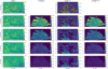 |
Fig. 3. ⟨Rdiag⟩ depending on the size of the local calibration. From top to bottom, calibration is done on 0.25, 0.5, 1, 2, 4 deg2. The four columns are |


5.4.2. Variation of the additive bias
The additive bias and its standard deviation are shown in Fig. 4. The standard deviation is as large as the value itself for local calibration on small scales. Except for the largest sub-patch sizes, the values of c1 and c2 per pixel are consistent with zero. This reflects the large fluctuations and randomness of the additive bias on small scales. To emphasize these conclusions, the 1D distributions of c1 and c2 are plotted in Fig. A.2.
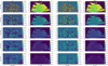 |
Fig. 4. c1 and c2 depending on the size of the local calibration. From top to bottom, calibration is done on 0.25, 0.5, 1, 2, 4 deg2. The four columns are c1, its standard deviation, c2, and its standard deviation. |
5.4.3. Relative errors
We computed the errors of the response matrices at different sub-patch sizes, averaged over all sub-patches (blue lines), compared to the relative errors of the global calibration (black lines). The results are shown in Fig. 5.
 |
Fig. 5. Relative errors of shear matrix (left panel) and selection matrix (right panel). In both cases, the blue line is the relative error of the diagonal terms of the matrix depending on the calibration size. The black line is the relative error of the diagonal terms of the matrix computed with the value obtained on the global calibration case. |
The relative error of the shear matrix is below 1% in all cases but always above the relative error of the global calibration, meaning that there are fluctuations at all the studied scales, but these are small. The fractional error of the selection matrix is higher. It reaches 17% at small sub-patch sizes but decreases up to 3% at 4 deg2. For the shear and selection matrix, we see that when we go on a smaller calibration size, the relative errors asymptotically approach the one of the global calibration.
5.5. Parameter correlation matrix
The calculation of the local shear bias allows us to further explore possible origins of shear bias, and their influence on other quantities obtained from the galaxy sample. To that end, we computed the correlation matrix between different quantities, for which we used patches of size ds = 1 deg. We also considered correlations between quantities other than shear bias. The correlation matrix is calculated using the pandasDataFrame.corr function12; it uses the Pearson method, which computes the standard correlation coefficient. The correlation matrix between the different quantities listed in Table 3 is shown in Fig. 6. To better see the correlation terms by terms, another correlation matrix is shown in Fig. B.1.
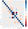 |
Fig. 6. Correlation matrix of the quantities listed in Table 3. The colors indicate the amplitude of the correlation, ranging between −1 and 1. All quantities are mean values. |
First, we see that the E- and B-mode smoothed convergence, κE, sm and κB, sm, are not strongly correlated. This indicates that there is no significant systematic effect that mixes both modes. Neither mode is strongly correlated to other quantities. Also, the number of peaks npeak is not correlated to observational effects.
Further, there is no visible correlation between the PSF size and the additive bias. This is evidence for the correct estimation of PSF size since a bias in the PSF size typically leads to an additive shear bias. We also note the absence of a correlation between the PSF ellipticity and the shear selection matrix. This gives us confidence that the PSF deconvolution in the metacalibration process works well. There is, however, a 20–30% negative correlation between the selection response elements and the size of the PSF. A plausible explanation is that in areas with larger seeing, fewer small and faint galaxies make it into the weak-lensing sample. This leads to a stronger (more negative) selection bias, which is reflected in the anticorrelation.
A negative correlation can be seen between the number of epochs, nepoch, and the PSF ellipticity modulus |ePSF|. Since the former is the mean over all contributing epochs, a reason for this anticorrelation might be the PSF ellipticity gets more circular when averaged over more independent observations.
There is a negative correlation of the r-band magnitude with galaxy weight w, S/N, and size Tgal, as well as a positive correlation with nepoch. This reflects the expectation that faint galaxies have a lower weight and S/N, and are easier observed with more exposures.
6. Impact of uncertainty and systematic effects on cosmological parameters
This section explores different systematic effects and uncertainties, and their impact on cosmological parameter constraints. We quantify the potential biases on cosmology from the spatially varying shear calibration (Sect. 6.1), the redshift uncertainty (Sect. 6.3), a residual shear bias (Sect. 6.2), baryonic feedback (Sect. 6.4), intrinsic galaxy alignment and cluster member dilution (Sect. 6.5). All these effects are studied jointly in Sect. 6.6.
For each effect, we will show constraints on cosmological parameters as compared to those obtained with the “ideal” case. This case, which is represented in blue in all the following figures represents the constraints obtained when we use the data calibrated globally without residual shear bias, a mean redshift of  , without baryonic correction, cluster member dilution or intrinsic alignment. This assumes an unrealistic best-case scenario of vanishing spatial variation of shear calibration and residual shear bias, and no biases from baryons, intrinsic alignment or cluster members. When the parameters are well-constrained, we specify the shift compared to the ideal case, which is the case for Ωm. The parameters Mν and the lower bound for As are in most cases not well constrained within the prior.
6.1. Local calibration
To study the impact on cosmology of spatially varying shear biases, we performed a local shear calibration using different scales, following the method explained in Sect. 5.3 for the multiplicative shear bias. For the additive bias, we used the value obtained with the global calibration because the local calibration value is very noisy. The result is shown in Fig. 7. We see that a local calibration will always shift Ωm to a lower value except for the calibration on 0.5 deg2. These variations are all within the statistical error bars. There is no systematic variation that becomes evident when going to smaller calibration sizes. For As and ∑Mν, the trend is not clear. Ωm shifts by −0.015, which corresponds to −0.3σ (i.e., 0.3 times the statistical uncertainty) when the calibration goes from global to local on 4 deg2 for example.
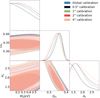 |
Fig. 7. 1D and 2D marginal posteriors for CFIS-P3 using different calibration sizes in the metacalibration. The 2D inner and outer contours show the 68% and 95.5% credible region, respectively. The case when the calibration is done globally (blue) is compared to the case where the calibration is done on 0.5 (black), 1 (green), 2 (red), and 4 deg2 (pink). Ωm shifts by −0.015, which corresponds to −0.3σ when the calibration goes from global to local on 4 deg2. |
From this work, it is not clear which calibration size is the best one because, depending on the size of the calibration, we will capture more or less the local effect. Future work has to be done to determine the criteria to choose the size of the calibration. In this work, when we need a local calibration, we use the one done on 1 deg2 because the relative error of the selection matrix (which is the limiting one) is below 10%.
6.2. Residual multiplicative shear bias
The shear bias m computed earlier with metacalibration is not perfect. A residual bias Δm = mmetacal − mtrue remains and generally has to be quantified with image simulations. We used the value Δm = 0.007 based on the results from Guinot et al. (2022), who found Δm = 0.007 ± 0.03, estimated using CFIS-like image simulations of isolated galaxies and ignoring the effect of blending. In comparison, other surveys also find residual biases at around the per cent level or below; for example, MacCrann et al. (2021) and Gatti et al. (2021) state a value of Δm = −0.0208 ± 0.0012 for DES-Y3.
We modeled the effect of the residual multiplicative shear bias by adding the residual bias Δm to the response matrix in the local case. This corresponds to a conservative, worst-case scenario where the residual bias is constant in space. Thus, Eq. (9) is modified to
 (14)
(14)
where I is the identity matrix. The impact of this bias on the cosmological constraints is shown in Fig. 8. In blue, the calibration is global whereas it is done on 1 deg2 for the green and red cases. Moreover, the red case includes the multiplicative shear bias. Including the residual shear bias changes the values of the parameters in the same direction as the local calibration compared to the global calibration. Ωm shifts by −0.024, which corresponds to −0.5σ with respect to the global calibration. A positive Δm effectively reduces the estimated shear, resulting on average in a smaller number of peaks, and thus smaller clustering parameters. The 1D marginalized contours for As shift to the right, contrary to what we would expect. However, the joint Ωm – As 2D contours clearly reflect the smaller calibrated shear and shift toward smaller clustering amplitudes.
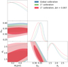 |
Fig. 8. 1D and 2D marginal posteriors for CFIS-P3, with the residual multiplicative shear bias added. The 2D inner and outer contours show the 68% and 95.5% credible region, respectively. Ωm shifts by −0.01, which corresponds to −0.2σ when the calibration goes from global (blue contour) to local on 1 deg2 (green contour). When Δm is added (red contour), Ωm shifts by −0.024, which corresponds to −0.5σ with respect to the global calibration. |
6.3. Redshift uncertainty
As discussed in Sect. 2.3,  is our best estimate of the redshift of the data observed from CFIS. This estimate has however a level of uncertainty. To quantify the impact of this uncertainty on our results, we compared cosmological constraints using the simulated convergence maps interpolated to
  and
and  , which corresponds to the two mean redshift estimates discussed in Sect. 2.3. The result is shown in Fig. 9. Fitting the data with the model at a higher mean redshift only slightly shifts the posterior: Ωm shifts by +0.001, which corresponds to +0.02σ when the redshift goes from 0.65 to 0.68. These shifts are well within the statistical uncertainties of the two parameters. Such a shift is, however, expected to have a significant influence on analyses using a larger survey area and/or redshift tomography. We also performed a test using only simulations, where the data vector was the mean of the fiducial simulation at z = 0.65 or at z = 0.68. The result is presented in Appendix C. We note, however, that when using simulations only, the shift appears to be larger, this may indicate some residual systematics that impacts the results on the data shown in this section.
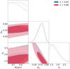 |
Fig. 9. 1D and 2D marginal posteriors using simulations at different redshift. The 2D inner and outer contours show the 68% and 95.5% credible region, respectively. The shear calibration is global. Ωm shifts by +0.001, which corresponds to +0.02σ when the redshift goes from 0.65 (blue) to 0.68 (red). |
6.4. Baryonic feedback
The impact of baryons on the LSS is important for cosmological analyses with weak-lensing peak counts (Osato et al. 2015; Harnois-Déraps et al. 2021b; Coulton et al. 2020). The redistribution of matter due to baryonic processes tends to reduce the number of high S/N peaks and augment that of smaller S/N values.
We used the results from Coulton et al. (2020) who model the fractional difference of the number of peaks, ΔNpeaks/Npeaks, for three different baryon physics scenarios based on the BAHAMAS hydrodynamical simulations (McCarthy et al. 2016) compared to MassiveNuS dark-matter-only simulations (Liu et al. 2018). This assumes that baryonic processes are independent of the underlying cosmology. The three scenarios are denoted as LowAGN, Fiducial, and HighAGN, where the amount of baryonic feedback increases in that order. The fiducial baryonic correction comes from the BAHAMAS simulations with a feedback model designed to best match the observations. The LowAGN and HighAGN corrections are simulations where the active galactic nucleus (AGN) heating is lowered or raised by 0.2 dex, respectively, and thus the simulations skirt the lower and upper bounds of the observed gas fraction.
We modified the model predictions of peak counts by multiplying the number of peaks from the MassiveNuS (dark-matter-only) simulations by Npeaks/Npeaks, DM, shown in Fig. 10.
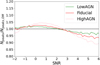 |
Fig. 10. Fractional difference in peak count obtained with Coulton et al. (2020) data. The difference between simulations with LowAGN, Fiducial, or HighAGN and dark-matter-only simulations is presented in green, red, and pink, respectively. |
We can see how the constraints evolve when we use real CFIS-P3 data and corrected simulations. To see the effect of the baryonic correction only, we use the global calibration, simulations at z = 0.65, no intrinsic alignment or cluster member dilution correction. We do not know how the baryonic feedback influences the observed data thus we correct the MassiveNuS simulations with the three different baryonic feedback corrections. In Fig. 11 we show the results of these corrections (LowAGN in green, Fiducial in red, and HighAGN in pink) compare to the case of the dark-matter-only simulation (blue).
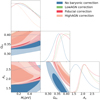 |
Fig. 11. 1D and 2D marginal posteriors for CFIS-P3, with the peak count predictions corrected with different baryonic feedback. The 2D inner and outer contours show the 68% and 95.5% credible region, respectively. The case without baryonic correction (blue) is compared to the three baryonic scenarios: LowAGN (green), Fiducial (red), and HighAGN (pink). Ωm shifts by +0.027, which corresponds to +0.5σ when the fiducial goes from dark-matter-only to LowAGN correction. |
Baryonic feedback has a significant impact on the best-fit parameters. Ωm and As are shifted to higher values with increasing baryonic modifications. For example, Ωm shifts by +0.027, which corresponds to +0.5σ when the fiducial goes from dark-matter-only to LowAGN correction. Li et al. (2019) found that it is the high S/N peaks that dominate the constraints and in Fig. 10 we see that the number of high peaks is suppressed by the baryonic feedback. This results in a shift toward higher values in Ωm, compensating for the suppression of peaks for S/N > 3. We also see that the strength of the feedback is not as important as just taking it into account.
6.5. Further systematic effects
At least two further effects can affect constraints: intrinsic alignment and cluster member dilution. As we briefly explain below, both effects can be suppressed, in first approximation, following Harnois-Déraps et al. (2021a), with a cut in S/N.
6.5.1. Intrinsic alignment
Due to the radial alignment of satellite galaxies within dark-matter halos, galaxies are not randomly oriented. Thus, their shape and alignments are affected by their environment and tidal fields. The intrinsic alignment has two components: the intrinsic-intrinsic correlations caused by the alignment of galaxies that are physically linked together and the gravitational-intrinsic correlations, which is the alignment of halo galaxies.
6.5.2. Cluster member dilution
The source density is not homogeneous and increases around foreground clusters. Around a cluster at a given redshift, there are more galaxies but, as we do not know their redshift, they are included in the signal but may not lensed. This effect leads to a coupling between the peak positions and the amplitude of the measured shear relative to the expected shear (Kacprzak et al. 2016). Moreover, these regions of clusters have a larger blending rate, and thus galaxies behind clusters are more likely to be missed. These effects can result in a miscalibration between data and simulations and lead to a reduction in the mean shear signal (as we count more galaxies for the signal). An analysis of cluster member dilution in Subaru HSC weak-lensing mass maps is available, for example, in Oguri et al. (2021).
6.5.3. Reducing intrinsic alignment and cluster member dilution with a cut on S/N
Harnois-Déraps et al. (2021a) find that the effect of intrinsic alignment is small for peaks with S/N < 3 and that the effect of the cluster member dilution is small for S/N < 4. The local calibration might capture part of the cluster dilution effect, but as we have no way of knowing it without simulations, we chose to cut the S/N range to be conservative. Thus, as a first approximation of how these effects impact the cosmological parameters, we computed the constraints using only the range for peak counts of S/N < 3. This selection should minimize the impact of both systematic contaminations. We tested both cases (−2 < S/N < 3 and −2 < S/N < 6) on mock peaks from MassiveNuS and find consistent results.
The comparison of the resulting constraints obtained with S/N < 3 (red) or S/N < 6 (blue) is shown in Fig. 12. Constraints are slightly larger when we cut the S/N range, which is expected. For both Mν and As parameters, the change is small.
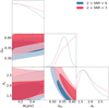 |
Fig. 12. 1D and 2D marginal posteriors for CFIS-P3 using different ranges in S/N. The 2D inner and outer contours show the 68% and 95.5% credible region, respectively. The shear calibration is global. The case with the full S/N range (blue) is compared to the case where we use −2 < S/N < 3 to minimize the effect of residual bias (red). Ωm shifts by +0.027, which corresponds to +0.5σ when we cut the high S/N peaks. |
The high-S/N peaks are affected by intrinsic alignment and cluster member dilution, which leads to a reduction in peak S/N (Harnois-Déraps et al. 2021a). When using the full S/N range and not accounting for those two effects, the reduction in peak S/N results in a lower inferred clustering amplitude and a lower Ωm. This can be seen in the Ωm – As 2D posterior distribution. We also perform a test using simulations only, with the range for peak counts of S/N < 3. As in previous tests, the data vector is the mean of the fiducial simulation at z = 0.65 and the result is presented in Appendix C.
6.6. Parameter constraints that combine all systematic effects
Our conservative model, which is the most suitable to represent the data, combines different mitigation schemes, and uses the following parameters and settings: The mean redshift is set to  . We calibrate the shear locally at a scale of 1 deg2. This accounts for spatial variations of shear bias and is the smallest scale for which the estimate of the selection is not dominated by noise. The residual shear bias is set to the value estimated from image simulations, Δm = 0.007. Baryonic feedback is accounted for by using the “fiducial baryon” case of Coulton et al. (2020). The data vector is composed of peak counts with −2 < S/N < 3 to minimize the systematic errors from intrinsic alignment and cluster member dilution.
In Fig. 13 we show constraints using this conservative model, and compare those to the ones obtained under the ideal (optimistic) case described at the beginning of this section. Ωm shifts by +0.008, which corresponds to +0.2σ when we go from the ideal to the conservative model. As expected, the conservative model results in wider constraints. In Fig. 14, we can see the marginalized distributions for the 68% confidence interval of the different parameters depending on the different cases we have tested.
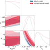 |
Fig. 13. 1D and 2D marginal posteriors for CFIS-P3 using the ideal or conservative model. The 2D inner and outer contours show the 68% and 95.5% credible region, respectively. The ideal one (blue) is obtained with global calibration, no baryonic correction, no intrinsic alignment, no boost factor, and on −2 < S/N < 6. The conservative model (red) is obtained with local calibration on 1 deg2, with residual bias, modeled under the fiducial baryonic correction, and on −2 < S/N < 3. Both models are computed at |

7. Conclusions
This study highlights the importance of properly accounting for systematics, such as the local calibration, residual multiplicative shear bias, intrinsic alignment and cluster member dilution, redshift uncertainties, and baryonic corrections, in the context of a peak-count cosmological analysis with CFIS data. We performed a likelihood analysis on the sum of neutrino masses, ∑Mν, the matter density parameter, Ωm, and the amplitude of the primordial power spectrum, As. For this purpose, we used the CFIS-P3 catalog and the MassiveNuSN-body simulations because they have the advantage of providing us with a large set of cosmological models and different tomographic bins. First, we obtained constraints with simulations only to validate the methodology used to model the redshift uncertainty, baryonic feedback, intrinsic alignment, and cluster member dilution. We then used the CFIS-P3 data to quantify the effect of systematics on cosmological constraints. We remark that Ωm is the parameter that is constrained the most and is the most impacted by the systematics. As a summary plot, Fig. 14, which shows the marginalized distributions for the 68% confidence interval of the parameters per studied case. On the one hand, the baryonic corrections, the intrinsic alignment, and the cluster member dilution shift this parameter to higher values. On the other hand, a local calibration and a multiplicative shear bias Δm = 0.007 shift Ωm to smaller values. Concerning As, the baryonic correction and the addition of Δm shifts this parameter to higher values, whereas cutting the high S/N peaks shifts As to a lower value. For ∑Mν, the parameter is not constrained enough to allow for any conclusions to be drawn. More specifically, concerning the shear calibration, it is probable that a local one is preferred over a global one, as long as the error and standard deviation are small, because it accounts for the local effects of the catalog. Nevertheless, some work has to be done to determine which calibration size is the better one. We notice that using a calibration on 1 deg2 with a value of the residual multiplicative shear bias Δm = 0.007 shifts Ωm by −0.024 (−0.5σ) compared to the case in which a global calibration is applied. Choosing a reasonable calibration size and having a robust estimate of Δm is important for having a better estimate of the constraints. We note that the residual bias used here computed from image simulations neglected effects such as galaxy image blending. A more realistic estimate of Δm is necessary for future analyses of CFIS weak-lensing data.
 |
Fig. 14. Marginalized distributions for the 68% confidence interval for the three cosmological parameters for the different cases that include uncertainties and systematic effects. |
Concerning the uncertainty on the mean redshift estimate, for a bias of  as considered in this study, the impact on the constraints is small enough to not be considered: the shift in Ωm is only +0.001 (+0.02σ). Nevertheless, we are aware that further work is needed to have a more complete description of the redshift distribution and obtain more accurate constraints. Using simulations only, the shift in Ωm is larger, 0.7σ. This indicates that other effects in the data might lead to an underestimation of the actual shift.
To account for baryonic corrections, we considered three different flavors of baryonic feedback, labeled in this study as HighAGN, Fiducial, and LowAGN correction. We conclude that the specific flavor of baryonic feedback is less important than the difference between baryonic feedback and pure dark-matter models. Applying the LowAGN baryonic correction shifts Ωm by +0.027 (+0.5σ), showing the importance of modeling the baryonic feedback. Using a prediction of peak counts based on hydrodynamical simulations to model the baryonic feedback can help in getting more accurate constraints.
Then, we see that when we minimize the effect of the cluster member dilution and intrinsic alignment by only considering peaks with S/N < 3, the posterior on Ωm is subject to an offset of 0.027 (0.5σ) toward higher values. Using simulations that model these effects will significantly improve the constraints since a cut in the S/N range will no longer be necessary.
Finally, we computed a conservative model where we used the parameters and settings that are most representative of the data. This gives larger constraints on Mν, Ωm, and As.
We noticed that the value of Ωm in particular can shift a lot due to different systematics. Our aim in this paper is not to estimate the final reference cosmological parameters, but rather to investigate, for the first time with UNIONS and peak counts, the impact of some of the different systematics at play for this survey. Among all the systematics considered in this paper, we have shown that the one with the highest impact on Ωm is related to how baryonic corrections are implemented (Fig. 11); the choice of cut on the S/N (Fig. 12) also causes a substantial shift. Other systematics not considered here may further shift the final parameters. It is necessary to further pursue this effort to include other systematic effects, as well as to extend the way we incorporate the baryonic feedback in the analysis and the choice of the calibration size. The constraints will be more accurate when simulations are able to also model intrinsic alignment and cluster member dilution; hydrodynamical simulations that include baryonic feedback could further improve the robustness of the results. In the future, having access to simulations built for UNIONS will allow us to make more precise investigations of various sources of bias. We also expect constraints to become more reliable with future (larger) data catalogs, such as the full UNIONS data set, for which the current pipeline will provide a starting point.
Acknowledgments
This work is based on data obtained as part of the Canada-France Imaging Survey, a CFHT large program of the National Research Council of Canada and the French Centre National de la Recherche Scientifique. Based on observations obtained with MegaPrime/MegaCam, a joint project of CFHT and CEA Saclay, at the Canada-France-Hawaii Telescope (CFHT) which is operated by the National Research Council (NRC) of Canada, the Institut National des Science de l’Univers (INSU) of the Centre National de la Recherche Scientifique (CNRS) of France, and the University of Hawai’i. Pan-STARRS is a project of the Institute for Astronomy of the University of Hawai’i, and is supported by the NASA SSO Near Earth Observation Program under grants 80NSSC18K0971, NNX14AM74G, NNX12AR65G, NNX13AQ47G, NNX08AR22G, and by the State of Hawai’i. This work has made use of the CANDIDE Cluster at the Institut d’Astrophysique de Paris and was made possible by grants from the PNCG, CNES, and the DIM-ACAV. This work was supported in part by the Canadian Advanced Network for Astronomical Research (CANFAR) and Compute Canada facilities. We would like to thank the anonymous referee for their helpful suggestions that improved the manuscript. We would also like to thank Joachim Hernois-Déraps for various discussions, particularly about the local metacalibration method. We are further grateful to Jia Liu and William R. Coulton for useful discussions and for providing us with the baryonic corrections employed in the analysis. We would like to thank Santiago Casas for useful discussion. Finally, we would thank the Cosmostat members for discussions about different aspects of this project. We thank the Columbia Lensing group (http://columbialensing.org) for making their simulations available. The creation of these simulations is supported through grants NSF AST-1210877, NSF AST-140041, and NASA ATP-80NSSC18K1093. We thank New Mexico State University (USA) and Instituto de Astrofisica de Andalucia CSIC (Spain) for hosting the Skies & Universes site for cosmological simulation products. Finally, this work uses the following software packages: astropy, numpy, jupyter, matplotlib, sklearn, scipy, emcee, chainconsumer, getdist, os and sys.
References
- Ajani, V., Peel, A., Pettorino, V., et al. 2020, Phys. Rev. D, 102, 103531 [Google Scholar]
- Ajani, V., Starck, J.-L., & Pettorino, V. 2021, A&A, 645, L11 [NASA ADS] [CrossRef] [EDP Sciences] [Google Scholar]
- Allys, E., Marchand, T., Cardoso, J.-F., et al. 2020, Phys. Rev. D, 102, 103506 [NASA ADS] [CrossRef] [Google Scholar]
- Bartelmann, M., & Schneider, P. 2001, Phys. Rep., 340, 291 [Google Scholar]
- Chambers, K. C., Magnier, E. A., Metcalfe, N., et al. 2016, ArXiv e-prints [arXiv:1612.05560] [Google Scholar]
- Cheng, S., Ting, Y.-S., Ménard, B., & Bruna, J. 2020, MNRAS, 499, 5902 [Google Scholar]
- Coulton, W. R., Liu, J., Madhavacheril, M. S., Böhm, V., & Spergel, D. N. 2019, J. Cosmol. Astropart. Phys., 2019, 043 [CrossRef] [Google Scholar]
- Coulton, W. R., Liu, J., McCarthy, I. G., & Osato, K. 2020, MNRAS, 495, 2531 [Google Scholar]
- Cragg, C., Duncan, C. A. J., Miller, L., & Alonso, D. 2022, MNRAS, 518, 4909 [CrossRef] [Google Scholar]
- Dietrich, J. P., & Hartlap, J. 2010, MNRAS, 402, 1049 [Google Scholar]
- Fluri, J., Kacprzak, T., Refregier, A., et al. 2018, Phys. Rev. D, 98, 123518 [NASA ADS] [CrossRef] [Google Scholar]
- Fluri, J., Kacprzak, T., Lucchi, A., et al. 2022, Phys. Rev. D, 105, 083518 [NASA ADS] [CrossRef] [Google Scholar]
- Gaia Collaboration (Brown, A. G. A., et al.) 2018, A&A, 616, A1 [NASA ADS] [CrossRef] [EDP Sciences] [Google Scholar]
- Gatti, M., Chang, C., Friedrich, O., et al. 2020, MNRAS, 498, 4060 [Google Scholar]
- Gatti, M., Sheldon, E., Amon, A., et al. 2021, MNRAS, 504, 4312 [NASA ADS] [CrossRef] [Google Scholar]
- Guinot, A., Kilbinger, M., Farrens, S., et al. 2022, A&A, 666, A162 [NASA ADS] [CrossRef] [EDP Sciences] [Google Scholar]
- Gwyn, S. D. J. 2008, PASP, 120, 212 [Google Scholar]
- Harnois-Déraps, J., Martinet, N., & Reischke, R. 2021a, MNRAS, 509, 3868 [CrossRef] [Google Scholar]
- Harnois-Déraps, J., Martinet, N., Castro, T., et al. 2021b, MNRAS, 506, 1623 [CrossRef] [Google Scholar]
- Hildebrandt, H., Erben, T., Kuijken, K., et al. 2012, MNRAS, 421, 2355 [Google Scholar]
- Hildebrandt, H., Viola, M., Heymans, C., et al. 2016, MNRAS, 465, 1454 [Google Scholar]
- Hoekstra, H., Viola, M., & Herbonnet, R. 2017, MNRAS, 468, 3295 [NASA ADS] [CrossRef] [Google Scholar]
- Huff, E., & Mandelbaum, R. 2017, ArXiv e-prints [arXiv:1702.02600] [Google Scholar]
- Jain, B., & Waerbeke, L. V. 2000, ApJ, 530, L1 [NASA ADS] [CrossRef] [Google Scholar]
- Kacprzak, T., Kirk, D., Friedrich, O., et al. 2016, MNRAS, 463, 3653 [Google Scholar]
- Kaiser, N., & Squires, G. 1993, ApJ, 404, 441 [Google Scholar]
- Kitching, T. D., Deshpande, A. C., & Taylor, P. L. 2021, Open J. Astrophys., 4, 1 [NASA ADS] [Google Scholar]
- Kratochvil, J. M., Lim, E. A., Wang, S., et al. 2012, Phys. Rev. D, 85, 103513 [Google Scholar]
- Kruse, G., & Schneider, P. 1999, MNRAS, 302, 821 [Google Scholar]
- Kuchner, U., Ziegler, B., Verdugo, M., Bamford, S., & Häußler, B. 2017, A&A, 604, A54 [NASA ADS] [CrossRef] [EDP Sciences] [Google Scholar]
- Li, Z., Liu, J., Matilla, J. M. Z., & Coulton, W. R. 2019, Phys. Rev. D, 99, 063527 [Google Scholar]
- Lin, C.-A., & Kilbinger, M. 2015, A&A, 576, A24 [NASA ADS] [CrossRef] [EDP Sciences] [Google Scholar]
- Liu, J., & Haiman, Z. 2016, Phys. Rev. D, 94, 043533 [Google Scholar]
- Liu, X., Pan, C., Li, R., et al. 2015a, MNRAS, 450, 2888 [Google Scholar]
- Liu, J., Petri, A., Haiman, Z., et al. 2015b, Phys. Rev. D, 91, 063507 [Google Scholar]
- Liu, J., Bird, S., Matilla, J. M. Z., et al. 2018, J. Cosmol. Astropart. Phys., 2018, 049 [Google Scholar]
- MacCrann, N., Becker, M. R., McCullough, J., et al. 2021, MNRAS, 509, 3371 [CrossRef] [Google Scholar]
- Mandelbaum, R. 2018, ARA&A, 56, 393 [Google Scholar]
- Martinet, N., Schneider, P., Hildebrandt, H., et al. 2017, MNRAS, 474, 712 [Google Scholar]
- Massey, R., Hoekstra, H., Kitching, T., et al. 2012, MNRAS, 429, 661 [Google Scholar]
- McCarthy, I. G., Schaye, J., Bird, S., & Le Brun, A. M. C. 2016, MNRAS, 465, 2936 [Google Scholar]
- Miller, L., Heymans, C., Kitching, T. D., et al. 2013, MNRAS, 429, 2858 [Google Scholar]
- Newman, J. A., Cooper, M. C., Davis, M., et al. 2013, ApJS, 208, 5 [Google Scholar]
- Oguri, M., Miyazaki, S., Li, X., et al. 2021, PASJ, 73, 817 [NASA ADS] [CrossRef] [Google Scholar]
- Osato, K., Shirasaki, M., & Yoshida, N. 2015, ApJ, 806, 186 [Google Scholar]
- Parroni, C., Cardone, V. F., Maoli, R., & Scaramella, R. 2020, A&A, 633, A71 [NASA ADS] [CrossRef] [EDP Sciences] [Google Scholar]
- Paulin-Henriksson, S., Amara, A., Voigt, L., Refregier, A., & Bridle, S. L. 2008, A&A, 484, 67 [NASA ADS] [CrossRef] [EDP Sciences] [Google Scholar]
- Particle Data Group (Patrignani, C., et al.) 2016, Chin. Phys. C, 40, 100001 [NASA ADS] [CrossRef] [Google Scholar]
- Peel, A., Lin, C.-A., Lanusse, F., et al. 2017, A&A, 599, A79 [NASA ADS] [CrossRef] [EDP Sciences] [Google Scholar]
- Petri, A. 2016, Astron. Comput., 17, 73 [NASA ADS] [CrossRef] [Google Scholar]
- Petri, A., May, M., & Haiman, Z. 2016, Phys. Rev. D, 94, 063534 [Google Scholar]
- Pyne, S., & Joachimi, B. 2021, MNRAS, 503, 2300 [NASA ADS] [CrossRef] [Google Scholar]
- Shan, H., Liu, X., Hildebrandt, H., et al. 2017, MNRAS, 474, 1116 [Google Scholar]
- Sheldon, E. S., & Huff, E. M. 2017, ApJ, 841, 24 [NASA ADS] [CrossRef] [Google Scholar]
- Shirasaki, M., Moriwaki, K., Oogi, T., et al. 2021, MNRAS, 504, 1825 [NASA ADS] [CrossRef] [Google Scholar]
- Spindler, A. 2018, Ph.D. Thesis, The Open University [Google Scholar]
- Takada, M., & Jain, B. 2004, MNRAS, 348, 897 [Google Scholar]
- Troxel, M. A., & Ishak, M. 2015, Phys. Rep., 558, 1 [NASA ADS] [CrossRef] [Google Scholar]
- Van Waerbeke, L., Benjamin, J., Erben, T., et al. 2013, MNRAS, 433, 3373 [Google Scholar]
- Weinberg, D. H., Mortonson, M. J., Eisenstein, D. J., et al. 2013, Phys. Rep., 530, 87 [Google Scholar]
- Yang, X., Kratochvil, J. M., Wang, S., et al. 2011, Phys. Rev. D, 84, 043529 [Google Scholar]
- Zürcher, D., Fluri, J., Sgier, R., Kacprzak, T., & Refregier, A. 2021, J. Cosmol. Astropart. Phys., 2021, 028 [CrossRef] [Google Scholar]
- Zürcher, D., Fluri, J., Sgier, R., et al. 2022, MNRAS, 511, 2075 [CrossRef] [Google Scholar]
Appendix A: Variation of the response matrix and the additive bias
To have a better visualization of the variation of the response matrix and the additive bias, we compute the histogram of their distribution in Figs. A.1 and A.2, respectively. In every histogram, we add as a black line the value found by the global calibration. From those histograms, we can clearly see that when the pixels are smaller the dispersion is larger, which is because the number of galaxies in one patch is lower and therefore there is more noise. In all cases, we see that the values are spread around the mean one.
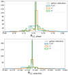 |
Fig. A.1. Histogram of R11, shear (top) and R11, selection (bottom) depending on the size of the local calibration. |
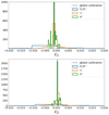 |
Fig. A.2. Histogram of c1 (top) and c2 (bottom) depending on the size of the local calibration. |
We confirm that the values are spread around the mean one, with larger dispersion at smaller scale of calibration.
Appendix B: Correlation matrix
The correlation matrix presented in Fig. B.1 is presented to see the correlation between the individual elements of the matrices.
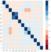 |
Fig. B.1. Correlation matrix of the quantities described in Sect. 5.1 or listed in Table 3. The colors indicate the amplitude of the correlation, ranging between −1 and 1. |
We can observe a strong correlation ( 60 - 80%) between  and
and  , which is expected because if the shear comports a bias, both component will be impacted. A correlation of 20 - 40% between
  and
and  is seen for the same reason as the correlation between
  and
and  . The
. The  and
and  are anticorrelated ( 20 - 40%) with the size of the psf Tpsf because if the psf is larger, we will miss more objects. Thus, the correlation effect is stronger.
Appendix C: Impact of the systematics using only simulations
As the data contain different systematics that are sometimes hard to model precisely, we perform some tests, using simulations only. The data vector is the mean of peak counts at the fiducial cosmology, which we modified to include systematics. The model used in the MCMC is the simulations at z = 0.65 without any modification. For every test, we compare the result to a data vector without any modification (blue of every figure).
C.1. Redshift uncertainty
The impact of the redshift uncertainty is shown in Fig. C.1, where we compute the data vector at z = 0.65 (blue) or z = 0.68 (red), whereas the model is kept at z = 0.65 in both cases. Modeling with lower redshift shifts Ωm by +0.7σ.
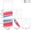 |
Fig. C.1. 1D and 2D marginal posteriors using as data the mean fiducial from the simulations at different redshifts. The 2D inner and outer contours show the 68% and 95.5% credible region, respectively. Ωm shifts by +0.026, which corresponds to +0.7σ when the redshift goes from 0.65 (blue) to 0.68 (red). |
C.2. Intrinsic alignment and cluster member dilution
The method used here to decrease the impact of intrinsic alignment and cluster member dilution is to cut the high S/N range. In Fig. C.2, we show the constraints when we use a S/N range between −2 and 6 (blue) or a reduced S/N range between −2 and 3 (red). When the reduced range is used, the constraints are larger, which is expected because there is less information.
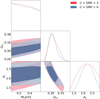 |
Fig. C.2. 1D and 2D marginal posteriors using as data the mean fiducial from the simulations and different ranges in S/N. The 2D inner and outer contours show the 68% and 95.5% credible region, respectively. The shear calibration is global. The case with the full S/N range (blue) is compared to the case where we use −2< S/N < 3 to minimize the effect of residual bias (red). The constraints are larger when we cut the high S/N peaks. |
All Tables
Mean redshift, , of CFIS weak-lensing galaxies for different redshift distributions, n(z), and maximum redshifts, zmax.
All Figures
|
Fig. 1. Convergence map of the CFIS-P3 patch. The squares indicate the regions free of large masks, which were used to compute the peak count. The total peak count is the mean of the peaks over the 13 patches. |
| In the text | |
|
Fig. 2. S/N map and peak counts histogram. The left plot is the S/N map of a part of the 512 × 512 pixels of CFIS-UNIONS data. The right plot is the peak counts computed on that S/N map. |
| In the text | |
|
Fig. 3. ⟨Rdiag⟩ depending on the size of the local calibration. From top to bottom, calibration is done on 0.25, 0.5, 1, 2, 4 deg2. The four columns are |
| In the text | |
|
Fig. 4. c1 and c2 depending on the size of the local calibration. From top to bottom, calibration is done on 0.25, 0.5, 1, 2, 4 deg2. The four columns are c1, its standard deviation, c2, and its standard deviation. |
| In the text | |
|
Fig. 5. Relative errors of shear matrix (left panel) and selection matrix (right panel). In both cases, the blue line is the relative error of the diagonal terms of the matrix depending on the calibration size. The black line is the relative error of the diagonal terms of the matrix computed with the value obtained on the global calibration case. |
| In the text | |
|
Fig. 6. Correlation matrix of the quantities listed in Table 3. The colors indicate the amplitude of the correlation, ranging between −1 and 1. All quantities are mean values. |
| In the text | |
|
Fig. 7. 1D and 2D marginal posteriors for CFIS-P3 using different calibration sizes in the metacalibration. The 2D inner and outer contours show the 68% and 95.5% credible region, respectively. The case when the calibration is done globally (blue) is compared to the case where the calibration is done on 0.5 (black), 1 (green), 2 (red), and 4 deg2 (pink). Ωm shifts by −0.015, which corresponds to −0.3σ when the calibration goes from global to local on 4 deg2. |
| In the text | |
|
Fig. 8. 1D and 2D marginal posteriors for CFIS-P3, with the residual multiplicative shear bias added. The 2D inner and outer contours show the 68% and 95.5% credible region, respectively. Ωm shifts by −0.01, which corresponds to −0.2σ when the calibration goes from global (blue contour) to local on 1 deg2 (green contour). When Δm is added (red contour), Ωm shifts by −0.024, which corresponds to −0.5σ with respect to the global calibration. |
| In the text | |
|
Fig. 9. 1D and 2D marginal posteriors using simulations at different redshift. The 2D inner and outer contours show the 68% and 95.5% credible region, respectively. The shear calibration is global. Ωm shifts by +0.001, which corresponds to +0.02σ when the redshift goes from 0.65 (blue) to 0.68 (red). |
| In the text | |
|
Fig. 10. Fractional difference in peak count obtained with Coulton et al. (2020) data. The difference between simulations with LowAGN, Fiducial, or HighAGN and dark-matter-only simulations is presented in green, red, and pink, respectively. |
| In the text | |
|
Fig. 11. 1D and 2D marginal posteriors for CFIS-P3, with the peak count predictions corrected with different baryonic feedback. The 2D inner and outer contours show the 68% and 95.5% credible region, respectively. The case without baryonic correction (blue) is compared to the three baryonic scenarios: LowAGN (green), Fiducial (red), and HighAGN (pink). Ωm shifts by +0.027, which corresponds to +0.5σ when the fiducial goes from dark-matter-only to LowAGN correction. |
| In the text | |
|
Fig. 12. 1D and 2D marginal posteriors for CFIS-P3 using different ranges in S/N. The 2D inner and outer contours show the 68% and 95.5% credible region, respectively. The shear calibration is global. The case with the full S/N range (blue) is compared to the case where we use −2 < S/N < 3 to minimize the effect of residual bias (red). Ωm shifts by +0.027, which corresponds to +0.5σ when we cut the high S/N peaks. |
| In the text | |
|
Fig. 13. 1D and 2D marginal posteriors for CFIS-P3 using the ideal or conservative model. The 2D inner and outer contours show the 68% and 95.5% credible region, respectively. The ideal one (blue) is obtained with global calibration, no baryonic correction, no intrinsic alignment, no boost factor, and on −2 < S/N < 6. The conservative model (red) is obtained with local calibration on 1 deg2, with residual bias, modeled under the fiducial baryonic correction, and on −2 < S/N < 3. Both models are computed at |
| In the text | |
|
Fig. 14. Marginalized distributions for the 68% confidence interval for the three cosmological parameters for the different cases that include uncertainties and systematic effects. |
| In the text | |
|
Fig. A.1. Histogram of R11, shear (top) and R11, selection (bottom) depending on the size of the local calibration. |
| In the text | |
|
Fig. A.2. Histogram of c1 (top) and c2 (bottom) depending on the size of the local calibration. |
| In the text | |
|
Fig. B.1. Correlation matrix of the quantities described in Sect. 5.1 or listed in Table 3. The colors indicate the amplitude of the correlation, ranging between −1 and 1. |
| In the text | |
|
Fig. C.1. 1D and 2D marginal posteriors using as data the mean fiducial from the simulations at different redshifts. The 2D inner and outer contours show the 68% and 95.5% credible region, respectively. Ωm shifts by +0.026, which corresponds to +0.7σ when the redshift goes from 0.65 (blue) to 0.68 (red). |
| In the text | |
|
Fig. C.2. 1D and 2D marginal posteriors using as data the mean fiducial from the simulations and different ranges in S/N. The 2D inner and outer contours show the 68% and 95.5% credible region, respectively. The shear calibration is global. The case with the full S/N range (blue) is compared to the case where we use −2< S/N < 3 to minimize the effect of residual bias (red). The constraints are larger when we cut the high S/N peaks. |
| In the text | |
Current usage metrics show cumulative count of Article Views (full-text article views including HTML views, PDF and ePub downloads, according to the available data) and Abstracts Views on Vision4Press platform.
Data correspond to usage on the plateform after 2015. The current usage metrics is available 48-96 hours after online publication and is updated daily on week days.
Initial download of the metrics may take a while.