| Issue |
A&A
Volume 670, February 2023
|
|
|---|---|---|
| Article Number | A34 | |
| Number of page(s) | 12 | |
| Section | Cosmology (including clusters of galaxies) | |
| DOI | https://doi.org/10.1051/0004-6361/202245198 | |
| Published online | 02 February 2023 | |
Reconstruction of weak lensing mass maps for non-Gaussian studies in the celestial sphere
AIM, CEA, CNRS, Université Paris-Saclay, Université de Paris, 91191 Gif-sur-Yvette, France
e-mail: This email address is being protected from spambots. You need JavaScript enabled to view it.
Received:
12
October
2022
Accepted:
20
December
2022
Abstract
We present a novel method for reconstructing weak lensing mass or convergence maps as a probe to study non-Gaussianities in the cosmic density field. While previous surveys have relied on a flat-sky approximation, forthcoming Stage IV surveys will cover such large areas with a large field of view (FOV) to motivate mass reconstruction on the sphere. Here, we present an improved Kaiser-Squires (KS+) mass inversion method using a HEALPix pixelisation of the sphere while controlling systematic effects. As in the KS+ methodology, the convergence maps were reconstructed without noise regularisation to preserve the information content and allow for non-Gaussian studies. The results of this new method were compared with those of the Kaiser-Squires (KS) estimator implemented on the curved sky using high-resolution realistic N-body simulations. The quality of the method was evaluated by estimating the two-point correlation functions, third- and fourth-order moments, and peak counts of the reconstructed convergence maps. The effects of masking, sampling, and noise were tested. We also examined the systematic errors introduced by the flat-sky approximation. We show that the improved Kaiser-Squires on the sphere (SKS+) method systematically improves inferred correlation errors by ∼10 times and provides on average a 20–30 % better maximum signal-to-noise peak estimation compared to Kaiser-Squires on the sphere (SKS). We also show that the SKS+ method is nearly unbiased and reduces errors by a factor of about 2 and 4 in the third- and fourth-order moments, respectively. Finally, we show how the reconstruction of the convergence field directly on the celestial sphere eliminates the projection effects and allows the exclusion or consideration of a specific region of the sphere in the processing.
Key words: gravitational lensing: weak / methods: data analysis
© The Authors 2023
 Open Access article, published by EDP Sciences, under the terms of the Creative Commons Attribution License (https://creativecommons.org/licenses/by/4.0), which permits unrestricted use, distribution, and reproduction in any medium, provided the original work is properly cited.
This article is published in open access under the Subscribe-to-Open model. This email address is being protected from spambots. You need JavaScript enabled to view it. to support open access publication.
1. Introduction
Gravitational lensing is the deflection of light rays from distant sources by massive objects along the line of sight (see, for example, Bartelmann & Schneider 2001). The apparent shape of the source becomes distorted when the light ray is coherently distorted by the gravitational field of the matter acting as the lens. In a weak lensing regime, where deflection angles are small, distortions in the image can be divided into two parts: shear, which distorts the shape of the source, and convergence, which isotropically magnifies or demagnifies it. The measurement of these deformations offers an absolute gravitational probe for the total distribution of matter in the Universe (together with dark matter) and can be used to statistically infer cosmological information. Until now, cosmological analyses based on weak lensing mainly relied on two-point estimators of the shear field (e.g. Schneider et al. 2002).
The most common approach is to compute a two-point shear correlation function from observational data (Kilbinger et al. 2013; Troxel et al. 2018; Hamana et al. 2020; Hikage et al. 2019; Asgari et al. 2021; Secco et al. 2022) or the shear power spectrum (Hikage et al. 2011, 2019; Heymans et al. 2012; Lin et al. 2012; Köhlinger et al. 2017; Camacho et al. 2022), and compare it with theoretical expectations. However, recently, cosmologists have become increasingly interested in extracting information from higher-order statistics such as peaks (e.g. Hilbert et al. 2012; Lin & Kilbinger 2015; Martinet et al. 2018, 2021a,b; Peel et al. 2017; Ajani et al. 2020; Ayçoberry et al. 2022), higher-order moments (e.g. Van Waerbeke et al. 2013; Petri et al. 2015; Vicinanza et al. 2016, 2018; Chang et al. 2018; Peel et al. 2017), and Minkowski functionals (e.g. Kratochvil et al. 2012; Petri et al. 2015; Vicinanza et al. 2019; Parroni et al. 2020; Zürcher et al. 2021). Although, theoretical predictions are more uncertain from these higher-order estimators. They are able to probe the non-Gaussian structure of the dark matter distribution and have proven to yield additional constraints (e.g. Liu et al. 2015; Liu & Hill 2015; Martinet et al. 2018; Harnois-Déraps et al. 2021). These non-Gaussian estimators are typically calculated from the convergence field beyond what can be obtained from the shear field, as the convergence maps are rich in information about the interaction between galaxies and clusters. However, the convergence is not directly observable and must be reconstructed from shear measurements. This has motivated research into optimal mass-mapping techniques.
Kaiser & Squires (1993) showed how to use weak lensing observable, shear measurements, to produce weak lensing convergence maps. This method is based on performing a direct Fourier inversion of the equations that relate the observed shear field to the convergence field, which is a scaled version of the integrated mass distribution. Indeed, the Kaiser-Squires (KS) method has been used to recover mass maps from a variety of recent weak lensing surveys, the Canada-France-Hawaii Telescope Lensing Survey (CFHTLenS1; Heymans et al. 2012) and the Dark Energy Survey (DES2; Flaugher et al. 2015) Science Verification (SV) data (respectively, Massey et al. 2007; Van Waerbeke et al. 2013; Chang et al. 2015). An important limitation of this approach is that it does not take into account noise (noise growth on small scales), mask, or boundary effects (in practice, the resultant mass map is smoothed to mitigate noise).
It should be noted that several alternative mass map reconstruction methods have been proposed to address the limitations of the KS method. Some of these proposed techniques include Wiener filtering (Jeffrey et al. 2018), sparsity priors (Pires et al. 2020), and others (Starck et al. 2021; Jeffrey et al. 2021). One key assumption of these ‘planar’ mass-mapping techniques is that a small field of view of the celestial sphere can be well approximated as a tangential planar projection onto the celestial sphere. This assumption is colloquially referred to as the flat-sky approximation. For small-field surveys, this approximation is typically justified. However, such an assumption will not be appropriate for ongoing – the Dark Energy Survey (Flaugher et al. 2015) and the Kilo Degree Survey (KiDS3; de Jong et al. 2013) – and upcoming – Nancy Grace Roman Space Telescope (formerly known as the Wide Field Infrared Survey Telescope4; Spergel et al. 2015), Euclid5 (Laureijs et al. 2011), and the Large Synoptic Survey Telescope (LSST6; LSST Science Collaboration 2009) – surveys, which will observe significant fractions of the celestial sphere. For future Stage IV wide-field surveys, mass mapping must be constructed natively on the sphere or inverted allowing for the spherical forward model to form the Spherical Kaiser-Squires (SKS) estimator to avoid errors due to projection effects. In general, the Kaiser-Squires method is a widely known approach but it is not robust to noise, field boundary effects, or survey masks on the shear fields.
In this paper, the previously developed improved Kaiser-Squire (KS+ Pires et al. 2020) formalism is extended to the sphere (henceforth referred to as SKS+). This paper is structured as follows. Section 2 describes the theoretical foundation of weak gravitational lensing, as well as data structures for spherical mapping, that is HEALPix and isotropic Undecimated Wavelet Transform on the Sphere (UWTS), following Bartelmann & Schneider (2001), Castro et al. (2005), Górski et al. (2005) and Starck et al. (2006). In Sect. 3 the full methodology that was used to generate the weak lensing convergence maps from shear, that is the reconstruction of weak lensing convergence maps using SKS and SKS+, is described. Section 5 describes the quality of the SKS+ method using a two-point correlation function, power spectrum, the third- and fourth-order moments, and peak statistics of the reconstructed convergence maps along with the effects of masking, sampling, and noise, and a comparison of the spherical case to the planar setting is provided. Concluding remarks are made in Sect. 6.
2. Formalism
2.1. Weak lensing on Sphere
We start by laying out the formalism for obtaining the full-sky convergence field κ as a set of spherical harmonics, constrained by observations of the shear γ field (e.g. Bartelmann & Schneider 2001; Castro et al. 2005; Chang et al. 2018).
In gravitational weak lensing, the lensing potential, ϕ, at 3D position in comoving space r ≡ (r, θ, φ) is defined by a surface integral over the 2D projected gravitational potential, Φ, along the line of sight (Bartelmann & Schneider 2001) as
 (1)
(1)
where coordinate r is a radial distance, (θ, φ) represents the angular position or spherical coordinates in the sky with colatitude θ ∈ [0, π] and longitude φ ∈ [0, 2π] and fK is a comoving angular diameter distance which depends on the curvature K of the universe.
The gravitational potential Φ is related to the matter overdensity, δ(r)≡δρ(r)/ρ by the Poisson equation:
 (2)
(2)
where the 3D gradient  is defined relative to the comoving coordinates, Ωm is the density of total matter to the present day, H0 is the Hubble constant today in units of km/s/Mpc, and a(t) = 1/(1 + z) is the scale factor.
The decomposition of the lensing potential (1) and its inverse into spherical harmonics is
 (3)
(3)
 (4)
(4)
where dΩ(θ, φ) = sin θ dθ dφ is the usual invariant measure on the sphere, Ylm are the spherical harmonics, ϕlm are the spherical harmonic coefficients and ⋆ denotes the complex conjugation, and l and m are the spherical harmonic degree and order, respectively.
Now, the spherical representation of the shear field can be defined as
 (5)
(5)
where the real component, γ1, represents the elongation along the x axis, and the compression along the y axis, γ2, represents a similar distortion, but rotated by +45°.
The convergence in terms of harmonics expansion of the lensing potential ϕ on the sphere can be written as
 (6)
(6)
where sYlm(θ, φ) is the spin-weighted spherical harmonic and s is its spin weight. The  and
and  are the spherical harmonic space coefficients associated with sYlm(θ, φ) at r7.
The equations for shear and convergence (Castro et al. 2005; Chang et al. 2018; Wallis et al. 2022; Pichon et al. 2010) are:
![Mathematical equation: $$ \begin{aligned}&{\hat{\gamma }_{lm}}{\,}_{\pm 2} \,= \, \hat{ \gamma }_{lm} = \hat{\gamma }_{E,lm} + i \hat{\gamma }_{B,lm} = \frac{1}{2} [l (l+1) (l-1) (l+2)]^{ \frac{1}{2}} \phi _{lm} \end{aligned} $$](/articles/aa/full_html/2023/02/aa45198-22/aa45198-22-eq10.gif) (7)
(7)
 (8)
(8)
From Eqs. (7) and (8), the derived relation between shear γ and convergence κ is represented as
 (9)
(9)
which is the spherical forward model, where  .
.
The E and B modes of the convergence field can be calculated by applying Eq. (9) on the spherical harmonics of shear.
In the flat sky limit, the decomposition into spherical harmonics is replaced by the Fourier transform,
 (10)
(10)
The above equations then reduce to the usual Kaiser & Squires (1993) formalism, and this mapping can be referred to as Spherical Kaiser-Squires (SKS).
2.2. HEALPix
Hierarchical Equal Area isoLatitude Pixelisation (HEALPix8; Górski et al. 2005) is a scheme to pixelize the curved sky. The aim of HEALPix is to support fast numerical analysis of data over the sphere. The notion is to support convolutions with local and global kernels, Fourier analysis with spherical harmonics, power spectrum estimation and topological analysis. The primary benefit of the HEALPix scheme is that all pixels have equal areas because the white noise generated by the signal receiver gets integrated exactly into the white noise in the pixel space. However, this comes at the cost of each pixel having a different shape.
The variable Nside parameter describes the resolution of HEALPix maps and also determines the number of pixels in the sphere as  ) of the same area
  . Throughout this article, the maps are constructed using Nside = 2048, corresponding to a pixel size of 1.7177 arcmin and all relevant spherical harmonic transforms use lmax = (3Nside − 1).
Spherical Harmonic Transforms9 are non-commutative Fourier transforms on the sphere. The HEALPix function map2alm is used to decompose the shear field into a spherical harmonic space obtaining the coefficients  ,
,  and calculate
  ,
,  according to Eq. (9). Finally, the HEALPix function alm2map is used to convert these coefficients back to the real-space κE and κB maps. The HEALPix routine anafast is used to estimate the power spectra of the maps.
2.3. Isotropic Undecimated Wavelet Transform on the Sphere
An Isotropic Undecimated Wavelet Transform on the Sphere (UWTS) based on spherical harmonics was described by Starck et al. (2006) that is used to reconstruct the wide field convergence maps. This isotropic transform is based on scaling function ϕlc(θ, φ) with cut-off frequency lc and which depends only on co-latitude θ and is invariant with respect to a change in longitude φ. The spherical harmonic coefficients ϕlc(l, m) of ϕlc vanish when m ≠ 0 which makes it simple to compute the spherical harmonic coefficients  of c0 = ϕlc * f, where * stands for convolution.
 (11)
(11)
Using this scaling function (ϕlc), it is possible to get a sequence of smoother approximations cj of the function f on a dyadic resolution scale. Let ϕ2−jlc be a rescaled version of ϕlc with cut-off frequency 2−jlc. Then the multiresolution decomposition cj can be obtained by convolving f with ϕ2−jlc
 (12)
(12)
where the zonal low pass filters hj are defined by
 (13)
(13)
The possible scaling function10 is 
 , where B3 is the cubic B-spline
 (14)
(14)
Just like with the à trous algorithm by Starck et al. (2010), the wavelet coefficients wj can be defined as the difference between two consecutive resolutions.
 (15)
(15)
which are equivalent to the wavelet function ψlc
 (16)
(16)
so that
 (17)
(17)
Since the wavelet coefficients are defined as the difference between two resolutions, the reconstruction from the wavelet decomposition W = {w1, …, wj, cj } is straightforward and corresponds to the reconstruction as of the à trous algorithm
 (18)
(18)
where the simplifying assumption has been made that f is equal to c0 and J represents the number of wavelet bands/scale.
3. Spherical mass inversion
In this section, the process of estimating the convergence map from an observed shear field on the sphere using SKS and SKS+ methods is discussed.
3.1. Kaiser-Squires on the sphere (SKS)
The reconstruction of the convergence map on the sphere from weak lensing involves solving a spherical inverse problem, as discussed above. In the weak lensing regime, the observational constraint can be fully expressed in terms of the reduced shear, g.
 (19)
(19)
However, when mapping the large-scale dark matter distribution within the weak regime, the reduced shear is approximately the true shear, γ ≃ g. Therefore, throughout the article, it has been avoided to perform reduced shear iterations.
This allows the observed shear to be
 (20)
(20)
where γn = γ + ϵs and ‘ϵs’ represent the shape noise described in Sect. 5.2, subscript ‘obs’ refers to the observations, γ the shear maps, and M is the mask (explained in Sect. 5.1 that correspond M = 1 when measurements(γn) have valid data and M = 0 indicating invalid data in observations. Therefore, Eq. (20) can be interpreted as a noisy measurement of true shear degraded by shape noise (caused by the unknown intrinsic ellipticities ‘ϵs’ of the observed galaxies) and Mask.
The KSK uses a spin transformation of the shear maps γ (γE and γB) to get both the curl-free E-mode convergence map κE, which carries most of the cosmological signal, and the divergence-free B-mode convergence map κB, which arises due to non-linear lensing corrections. The HEALPix functions are map2alm performs the decomposition of real space (γE and γB) into spherical harmonic spaces ( and
and  ) as in Eq. (9), which can be re-written as
 (21)
(21)
then alm2map converts the spherical harmonic space coefficients ( and
and  ) back to the real space maps (κE and κB). However, because this method does not account for noise and survey masks on the shear fields, poor results are inevitable.
3.2. Improved Kaiser-Squires on the sphere (SKS+)
In practice, due to the limitations of the observational quality i.e. noise (Sect. 5.2) and survey mask windows, where noise covariance is typically large in magnitude, the inverse problem become strongly ill-posed and thus significant regularisation is required to stabilise the inversion. The methods described in Pires et al. (2020) have been extended to the sphere in this paper to incorporate the necessary corrections for imperfect and realistic measurements. The convergence κ can be recovered by using a transformation Φ which yields κ = Φα. This deceptively simple expression requires some unpacking. In the spherical domain, the chosen dictionary Φ is denoted as the spherical harmonic basis, conversely ΦT is the spherical harmonic transform, i.e. the projector onto the spherical harmonic space. The vector α={ϕlm}l = 0, 1…lmax, m = −l, …, l is the set of spherical harmonic coefficients that reproduce the convergence, κ.
The extension of KS+ (Pires et al. 2020) can accommodate missing data to the celestial sphere. After applying SKS+, the missing data regions in the reconstructed convergence map and the corresponding shear maps have evolved to non-zero values. Then, following the essential idea of Pires et al. (2020), the best solution is identified from the set of all possible solutions as the sparsest, that is, the solution with the spherical harmonic coefficients, α.
The mass-inversion can be estimated by solving the following.
 (22)
(22)
where ∥ ⋅ ∥0 is the pseudonorm, that is, the number of non-zero entries in (⋅), ∥ ⋅ ∥ the classical l2 norm (i.e.  and σ stands for the noise standard deviation of the input shear map measured outside the mask. The solution to this convex optimisation problem can be obtained using an iterative thresholding process (Starck et al. 2004) and modifying it by multiplying the full residual by M after each residual estimation as in Abrial et al. (2008).
In ideal lens-source clustering (see Schneider et al. 2002), all astronomical weak lensing only approximately gives pure E modes and, in practice, observational effects, due either to an imperfect point-spread function correction or spatially varying calibration errors under the assumption that the PSF correction is correct or to an intrinsic alignment of galaxies arising from spin-spin correlation, induce B modes. The consequence is that any observational effects that would normally go into B modes are necessarily pumped into E modes. Thus the B-modes can provide an important check for systematic errors. In this paper, we force the B modes to zero inside the mask rather than letting them free, and we incorporate an additional constraint on the power spectrum of the convergence map as of Pires et al. (2020). The way this is implemented is using the Isotropic Undecimated Wavelet Transform on the Sphere. As described in Sect. 2.3, the idea is to decompose our image κ into a set of coefficients {w1, w2, …, wj, cj}, as a superposition of the form Eq. (18) (in this equation, f is equivalent to κ) where cj is a smoothed version of the image, and wj are a set of aperture mass maps (usually called wavelet bands) at scale θ = 2j. Aperture mass maps, wj, are obtained by convolving the image κ with 1D filter hj derived from the B3-spline as shown in Eqs. (13) and (14). Then, the variance of each wavelet band wj is estimated. The variance per scale estimated in this way can be directly compared to the power spectrum.
This provides a way to estimate a broadband power spectrum of the convergence κ from incomplete data. The power spectrum is then enforced by multiplying each wavelet coefficient by the factor  inside the gaps and then reconstructing the convergence through the inverse wavelet transform. The
  and
and  are the standard deviation estimated in the wavelet band wj inside and outside the mask, respectively.
After implying constraints, the Eq. (22) that we want to minimise can be re-written as
 (23)
(23)
1. Input: Shear map with mask in HEALPix format.
2. Compute κ by performing a direct spherical mass inversion. §3.1
3. Set the number of iterations Imax, the maximum threshold λmax = max(|α = ΦTκE|), and the minimum threshold λmin = 0.
4. Initialise solution: κ0 = 0
5. Set i to 0, λi = λmax and κi = κ. Iterate:
i Compute α = ΦTκi
ii Compute  by setting to zero the coefficients α below the threshold λi.
iii Reconstruct Κi from  : Κi = Φ
 .
.
iv Decompose  into its wavelet coefficients {w1,w2,......,wj,cj}.
v Renormalise the spherical wavelet coefficients wj by a factor  inside the gaps.
vi Reconstruct Κi by performing the backward spherical wavelet transform from the normalised coefficients.
vii Perform the inverse mass relation to compute γi
viii Enforce the observed shear γ outside the gaps: γi = (1 − M)γi + Mγ.
ix Perform the direct mass inversion and get κi
x Set i = i + 1.
xi Update the threshold: γi = F (i, γmin, γmax)
xii If i < Imax, return to step i.
where P is a linear operator to impose power spectrum constraint, W and WT are the forward wavelet transform and inverse wavelet transform on the sphere respectively (see Algorithm 111).
We quantified the quality of the reconstructed convergence maps with respect to missing data and shape noise in Sect. 5.
The function F fixes the decrease in the threshold, which decreases exponentially at each iteration from a maximum value to zero as described in Pires et al. (2009). F(i, λmin, λmax) = λmin + (λmax − λmin)(1 − erf(2.8 i/lmax)).
We applied this algorithm with around Imax = 100 iterations in the spherical harmonics representation. We estimated the relative mean squared error (MSE) for various Imax values to set this parameter. Figure 1 depicts the relative MSE per Imax and we discovered that the error does not decrease significantly after Imax > 90, so we used Imax = 100. We performed the test with other resolution maps and reached similar conclusions.
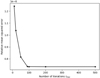 |
Fig. 1. Relative MSE as a function of maximum number of iterations Imax. |
4. Data
Convergence map reconstruction using the SKS+ method has been tested on several shear maps generated by high resolution and realistic N-body simulations (Takahashi et al. 2017)12. These simulation data sets are generated by performing multiple lens plane ray-tracing through high-resolution cosmological N-body simulations for redshifts zϵ[0.05, 5.3] at intervals of 150 h−1 Mpc comoving radial distance. Each box has 20483 Dark Matter particles, so the resolution is higher in boxes closer to the observer. The cosmological parameters selected for this suite of simulations are matter density Ωm = 1, cosmological constant ΩΛ = 0.279, baryon density Ωb = 0.046, Hubble parameter h = 0.7, normalisation σ8 = 0.82 and slope of the primordial power spectrum ns = 0.97. These parameters were adopted from standard cosmology ΛCDM (Lambda cold dark matter) that is consistent with the WMAP 9-year result (Hinshaw et al. 2013).
For the purpose of this article, shear maps at z = 2.9367 which is close to the current limits of the stage IV survey. Shear maps are available in HEALPix pixelisation with a resolution of Nside = 4096, which is degraded to a lower resolution map of Nside = 2048 by using the HEALPix ud_grade function (degrade by averaging the four input map pixels nested in one output map pixel value). Higher-resolution maps may produce better results at the cost of computational efficiency.
Finally, a pseudo-Euclid mask (masking of the stellar, galactic plane and the ecliptic), so as to best match upcoming Stage IV surveys like Euclid, has been applied to the shear maps as shown in Fig. 2.
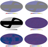 |
Fig. 2. Shear field is shown in the first and second columns of the upper panel (the first showing γ1 and the second showing γ2) with missing data. The first column of the middle panel shows the mask which applied to the shear maps and the second column shows the original E-mode convergence κ map. The lower panel shows the E-mode convergence maps reconstructed from the incomplete shear field using the SKS method (left), and using the SKS+ method (right). |
5. Quantifying the quality of reconstruction
This section discusses the impact of missing data, shape noise, and projection on the SKS and SKS+ inversion methods and provides quantitative evidence of the efficacy of the SKS+ method.
5.1. Missing data
Masking must be considered when analysing simulated data to more accurately represent real data. Real lensing datasets have gaps due to bad pixels or a defect in the camera’s CCD or the presence of a bright star in the field of view, which forces us to remove a part of the image. These gaps are usually described by a simple binary mask. These masked areas make post-processing difficult, especially when estimating statistical information such as the power spectrum.
In this paper, we use the mask that depicts the galactic plane, ecliptic plane, and stellar contamination; it mimics the setting of an upcoming Stage IV survey like Euclid to show how missing data can produce a significant systematic bias on clustering. We also show how our algorithm can accommodate a mask and effectively eliminate any bias. For this purpose, the Euclid-like mask is applied to the corresponding projected noise-free shear map, as shown in the upper panel of the Fig. 2. The reconstruction of the convergence map is done after masking. In this section, to demonstrate the effects of the missing data, shape noise effects are not considered.
The middle panel of the second column of Fig. 2 shows the input true convergence map and the first and second columns of the lower panel show the E-mode convergence map reconstructed from the noise-free shear map using SKS and SKS+ method respectively.
The non-local behaviour of the Kaiser-Squires reconstruction method over limited survey windows introduces masking effects due to unknown shear outside the survey mask in the reconstruction. These masking effects present themselves as additional noise in the reconstructed maps and result in significant leakage (i.e. leakage in the E mode) during mass inversion. The problem is reformulated taking into account additional assumptions in the SKS+ algorithm, which is defined in Sect. 3.2.
Figure 3 compares the residual maps (the pixel difference between the input true map and the reconstructed E-mode maps) of the SKS and the SKS+ methods outside the mask. From the residual maps, it can be seen that most of the features of the input convergence map have been recovered, except for the part of the map close to the edges of the mask with the SKS method. Here we try to quantify the effects of masks arising from the limited survey windows at different scales using the two-point correlation function and higher-order moments.
 |
Fig. 3. Missing data effects: Pixel difference outside the mask between the original E-mode convergence map and the reconstructed E-mode convergence map using the SKS method (left) and the SKS+ method (right); the inner box corresponds to a zoom of the field 10° ×10° with centre at (5, 28). |
5.1.1. 2PCF
The two-point correlation function represents the density of two-point distances in a given feature space. The basic weak lensing measurements are the shear two-point correlation function, ξ±, (2PCF) and its associated power spectrum, the most popular statistic used to capture the second-order statistic in the cosmic shear analyses.
Shear two-point correlation functions correlate γt/×, the tangential and cross components of shear, of two galaxies separated by an angle θ in the sky (Bartelmann & Schneider 2001). The two-point correlation function, ξ±, and the power spectrum, Cl, of the weak lensing convergence map κ can be used to estimate the shape and normalisation of the dark-matter power spectrum. The ξ± measured with the tree code Athena13 (Kilbinger et al. 2014), the estimators defined in Schneider et al. (2002), with 200 logarithmic angular bins in the range of 1.7 ≤ θ ≤ 200 arcmin.
The angular power spectra, Cl, which express the correlations between pairs of galaxy ellipticities in harmonic space, are computed from the original and reconstructed convergence maps using the anafast routine implemented in HEALPix without performing any prior smoothing of the maps.
The left panel of Fig. 4 compares the mean two-point shear correlation function, ξ+ (black), with the corresponding mean two-point convergence correlation function ξκE reconstructed using the SKS method (red) and using the SKS+ method (blue) from incomplete noise-free shear maps. The right panel of the Fig. 4 shows the power spectrum estimated from the original convergence map to the one reconstructed from the masked shear maps using the SKS and SKS+ methods. The estimation is done on the 10 simulated maps for angular resolution Nside = 2048 and only made outside the mask M.
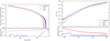 |
Fig. 4. Missing data effects: Mean shear two-point correlation function (black) with corresponding mean convergence two-point correlation function from SKS (red) and SKS+ (blue) reconstruction method (left panel) and power spectrum (right panel) from SKS (red) and SKS+ (blue) reconstruction method, from incomplete noise-free shear maps, compared to the original convergence map (black). The estimation is only made outside the mask M. The lower panel shows the relative errors introduced by the missing data effects, that is, the normalised difference between the upper curves. |
Figure 4 clearly show that the two-point correlation function of the SKS reconstruction (red) underestimates the power due to leakage in the shear B modes. The SKS+ map (blue) is a clear improvement over the SKS map and near perfect match to the original two-point correlation function (black). It is also notable that the SKS method under-predicts the power spectrum at large scales, due to mask effects and E-mode leakage. On the contrary, the SKS+ method recovers the power spectrum more accurately at all scales. The shaded area in both figures represents the error on the mean and the SKS+ falls within the 1σ uncertainty from the original estimations. It can be seen that SKS+ has ∼10 times fewer errors and systematic bias is negligible compared to the SKS method.
5.1.2. Moments
The moments test is an important and computationally less demanding tool for determining how well the reconstructed convergence maps preserve cosmological characteristics. The skewness of the convergence is sensitive to the cosmological matter density; however, the higher-order moments of the underlying dark matter density fields are much less sensitive to the background cosmological parameters (Jain et al. 2000). Skewness and kurtosis are also more direct estimators of signal non-Gaussianity.
We performed the wavelet decomposition using [sec:UWTS]UWTS of our convergence maps, original as well as the reconstructed maps of the mass distribution. For each wavelet scale, we have computed their third-order  and fourth-order
  moment outside the masks.
Figure 5 demonstrates that the SKS+ mass reconstruction method leads to reliable convergence maps with a discrepancy of less than 2% that preserves the statistical and cosmological information. The SKS errors rise with scale up to a factor of ∼3 and are less than 40% and less than 50% below 10″ and 100″, respectively. In contrast, SKS+ errors are substantially less noticeable on all scales and remain within uncertainty 1σ.
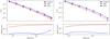 |
Fig. 5. Missing data effects: third-order (left panel) and fourth-order (right panel) E-mode moments of the original (black) compared to the moments estimated on the SKS (red) and SKS+ (blue) convergence maps on seven wavelet scale. The estimation of the moments is the average of the 10 simulated maps for angular resolution Nside = 2048 that is calculated outside the mask M. The lower panel shows the relative higher-order moment errors introduced by missing data effects, that is, the normalised difference between the upper curves. |
5.2. Weak lensing shape noise
The variance of intrinsic ellipticity, which is the dominant source of noise (ϵs), in shear measurements, causes ‘shape noise’. The convergence map is then affected by random noise that can be considered Gaussian with zero mean and variance  . Therefore, we consider the observational errors that are errors from ‘shape noise’ as expressed in Eq. (20).
The noise level of a given pixel in a weak lensing survey is determined by the following factors: the number density of galaxy observations ngal (typically given per arcmin2), the size of the said pixel, and the shape noise, the variance of the intrinsic ellipticity distribution,  . The variance for an ensemble follows Poisson statistics, so
  for an ensemble of N sources, or equivalently, knowing the area Apix of a given pixel with mean source density ng, the noise standard deviation σpix is simply given by
 (24)
(24)
where 3600( converts steradians to arcmin2 – this relation is simply a reduction in the noise standard deviation by the root of the number of data points. As a result, larger pixels that contain more observations (assuming a roughly uniform spatial distribution of galaxy observations) have lower noise variance. In practice, the true number of galaxies in a given pixel, rather than ngal, can be used to calculate the value of σpix.
In what follows, we assume a typical value of an intrinsic ellipticity standard deviation, σϵ ∼ 0.26, which is close to typical values for both ground-based and space-based observations (e.g. Leauthaud et al. 2007) and assume a source density, ngal ∼ 30 per arcmin2, which is roughly what is expected for Euclid (Laureijs et al. 2011), Roman (Spergel et al. 2015) and LSST (LSST Science Collaboration 2009).
Figure 6 displays the mean unsmoothed shear two-point correlation function (black) and power spectrum estimates from the unsmoothed convergence maps obtained from SKS and SKS+ methods. The estimation is performed on the 10 simulated maps for angular resolution Nside = 2048 and only made outside the mask M, in the presence of the shape noise.
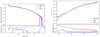 |
Fig. 6. Shape noise effects: Mean shear two-point correlation function (black) with corresponding mean convergence two-point correlation function from SKS (red) and SKS+ (blue) reconstruction method (left panel) and power spectrum (right panel) from SKS (red) and SKS+ (blue) reconstruction method compared to the original convergence map (black) with realistic shape noise. The estimation is only made outside the mask M. The lower panel shows the relative errors introduced by the missing data effects, that is, the normalised difference between the upper curves. |
In comparison with the left panel of the Figs. 4, 6 shows the less smooth two-point correlation function, caused by the noise fluctuations, which can be reduced simply by increasing the resolution of the HEALPix maps. However, the same findings are obtained that the SKS+ technique has fewer errors than the SKS technique and remains within the 1σ uncertainty.
Comparing Figs. 5 and 7, it can be seen that the fourth-order moment is biased at smaller scales. However, the SKS+ method is nearly unbiased and reduces errors by a factor of about 2 and 4 at the third and fourth-order moments, respectively. Furthermore, Fig. 7 represents that the higher-order moments beyond variance, namely skewness and kurtosis, surely preserve the cosmological information even in the presence of a realistic setting.
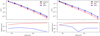 |
Fig. 7. Shape noise effects: third-order (left panel) and fourth-order (right panel) moments estimated on seven wavelet bands of the original E-mode convergence map with realistic shape noise (black) compared to the moments estimated on the SKS (red) and SKS+ (blue) convergence maps at the same scales. The SKS and SKS+ convergence maps are reconstructed from noisy shear maps. The estimation of the moments is the average of the 10 simulated maps for angular resolution Nside = 2048 that is calculated outside the mask M. The lower panel shows the relative higher-order moment errors introduced by shape noise. |
5.3. Peak counts
Peak counts are a simple and robust statistic that has received increasing attention in recent years (Maturi et al. 2010; Yang et al. 2011; Lin & Kilbinger 2015; Peel et al. 2017; Ajani et al. 2020; Ayçoberry et al. 2022), for accessing cosmological information from the non-Gaussianities in lensing fields. The peaks can be used as tracers of dark-matter halos, galaxy clusters, and lensing structure, and therefore the non-Gaussianities in the matter distribution. Therefore, the peaks are sensitive to the halo mass function and cosmological parameters (Marian et al. 2009; Shirasaki 2017). In this work, the focus is only on the study of peak counts, and the exploration of peak profiles and peak-correlation functions to improve cosmological constraints is left for further studies.
The peak count statistic is a straightforward evaluation that determines the number of peaks on the reconstructed convergence map as a function of their signal-to-noise ratio (SNR). Peak counting is accomplished by scanning pixels in a signal-to-noise field S/N, and looking for local maxima (i.e., pixels with a higher value of κ than its surrounding 8 pixels). A pixel is regarded as a peak if its value is higher than all the values of its neighbouring pixels. The get_all_neighbours function is used to search all neighbouring pixels. The number of peaks is then counted as a function of their centre value. Where S/N on the scale j is the ratio between the convergence κj and the standard deviation of the noise.
 (25)
(25)
In this case, the estimation of the standard deviation of the noise, σnoise, is performed on each wavelet scale, as described in Starck & Murtagh (1998). The κj is the set of aperture mass maps that are obtained by convolving κ with 1D filter hj as shown in Eq. (13). We transform κ with the wavelet scale J = 4 and identify the peaks on these maps. s
The features of the map have been grouped into bins of the signal-to-noise ratio (SNR) instead of κ, as has been done mainly in previous studies. The positive and negative peaks of the full sky convergence maps without tomographic decomposition are estimated outside the mask. Figure 8 shows the peak abundance as a function of the SNR. Peaks estimated on original and reconstructed convergence maps are shown in black, red (SKS) and blue (SKS+) respectively. The curves correspond to the mean over 10 simulated maps for angular resolution Nside = 2048. The SKS+ method provides on average 20–30% better peak estimation compared to the SKS method. It can be seen that the number of counts depends on the resolution, as expected, and the transform picks out features of the convergence map, κ, at successively larger scales as j increases. Figure 8 also shows the good agreement between the SKS+ and the original predictions on all wavelet filtering scales. It is also noteworthy that peak statistics are likely to be robust towards unknown errors in the galaxy ellipticities that complicate the use of field statistics. In principle, peak statistics encode information about dark matter halos, voids, and cluster structures, and therefore non-Gaussianities in matter distribution (Fan et al. 2010; Shirasaki 2017). Further work is required to evaluate the biasing of galaxies relative to dark matter by estimating the relation of galaxies to halos and the relation of halos to dark matter.
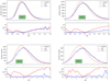 |
Fig. 8. Peak counts: Convergence map (black) to the Peaks estimated on the SKS (red) and SKS+ (blue) convergence maps over the wavelet coefficient maps {wj} up to jmax = 4. The plots show the average peaks of the 10 simulated maps for angular resolution Nside = 2048 and estimations are only made outside the mask M. |
5.4. Projection effects
As moving towards greater sky-coverage areas with near-future surveys, namely Euclid (15 000 deg2) and LSST (20 000 deg2) compared to DES (5000 deg2), it is necessary to understand the projection effects, take sky geometry into account, and encourage spherical analysis over planar approximation. Spherical projections onto the plane cannot preserve all the features of the spherical map, and these projection effects decrease the sensitivity to the clustering on small scales.
This section aims to understand the effects of projections; therefore, only noiseless maps are considered. Mapping the spherical projection from HEALPix to the plane or vice-versa results in distortion. When creating convergence maps on the plane, the exact projection used to map the celestial sphere to the plane can have an impact on the quality of the reconstructed convergence map. Since the resulting spherical harmonic transforms are theoretically exact, any errors will therefore be due to projection effects rather than inaccuracies in the harmonic transforms.
We compared the higher-order moment, estimates in the E-mode of the spherical convergence map and planar convergence maps as in Fig. 9. To investigate the distortions, there was an absolute need to partition the full-sky shear maps, with and without masks, into patches and, preferably, non-overlapping planar maps. In practice, the size of the patches plays an important role in obtaining noticeable projection effects. Therefore, we decompose the celestial sphere into square patches of 4 × 4 deg2 and 10 × 10 deg2 (centered on the centre of the planar map) in such a way that the induced distortions remain at a minimum and the pixel size corresponds to Nside = 2048. The projected HEALPix pixels of the flat maps are converted into standard square pixels using nearest-neighbour interpolation.
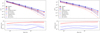 |
Fig. 9. Projection effects: Third-order (left panel) and fourth-order (right panel) moments estimated on seven wavelet bands of the original E-mode Convergence map (black solid line for full sky, black dashed line and black dotted line for planar approximation of 10° ×10° and 4° ×4° respectively) compared to the moments estimated on the SKS, SKS+ (red & blue solid lines respectively) and KS, KS+ (for planar, red and blue dashed and dotted lines respectively). The plots show the comparison of only one realisation for angular resolution Nside = 2048 and estimations are only made outside the mask M. |
The convergence field was estimated from this planar shear field using the planar KS (Kaiser & Squires 1993) and KS+ (Pires et al. 2020) estimators, and then compared these recovered planar convergences to the celestial sphere convergence field estimated using SKS (Sect. 3.1) and SKS+ (Sect. 3.2) methods.
As shown in Fig. 9, the pixelation effect biases the moments too much which is minimal for small and intermediate scales but more significant for the largest scales. This bias can be explained due to the projection distortion and the boundary created by the projection. It can be seen that convergence reconstruction on the celestial sphere not only reduces errors but is also easily generalised by replacing the usual flat-sky convergence reconstruction. However, due to the non-linear nature of the effect, induced by the projection remain at a 10% level on smaller scales.
We also test the projection effects by converting HEALPix pixels into standard square pixels using bi-linear interpolation and we didn’t find any significant difference.
Instead of just decomposing shear maps and performing KS and KS+, we also decomposed our convergence maps reconstructed from SKS and SKS+ methods, and we got the equivalent yet somewhat better results at small scales. Hence, we can say that by recovering weak lensing mass maps directly on the sphere and thereby eliminating the distortion due to a projection to the plane, the performance of reconstruction is enhanced. Reconstruction of the convergence field directly on the celestial sphere also allows us to consider or exclude the specific regions of the sphere.
6. Conclusion
In this work, a new method, SKS+, for reconstructing mass maps without noise regularisation from weak lensing shear observations has been discussed. The previously presented KS+ (Pires et al. 2020) reconstruction formalism is extended to the spherical setting, resulting in a spherical KS+ mass-mapping algorithm which refers to as the SKS+ method. Throughout the paper, the analysis is performed at a typically adopted angular band limit of lmax = 3 * Nside − 1 and Nside = 2048. A higher resolution can result in extremely high computational costs, whereas a lower resolution would destroy the data. SKS+ method, on the other hand, is applicable to any pixelisation of the sphere.
Section 3 described how one can recover convergence fields directly on the celestial sphere by adopting the SKS and SKS+ techniques. The effects of missing data, sampling, and shape noise were tested and compared on the SKS and SKS+ reconstructed convergence maps using two-point correlation, power spectrum, third-and fourth-order moments, and peaks in a realistic setting. It is shown that the SKS+ method outperforms and reduces errors compared to the SKS method and preserves the statistical and cosmological information. In the noise-free case, we show that the SKS+ method systematically improves the inferred correlation errors that are affected by the Euclidean mask ∼10 times compared to the SKS method. We also showed that the SKS method systematically underestimates the higher-order moments i.e. skewness and kurtosis at all scales and the SKS+ method is nearly unbiased. While after adding realistic noise, the SKS+ method reduces errors by a factor of about 2 and 4 in the third- and fourth-order moments, respectively. These measurements from convergence maps may provide important constraints on the cosmological parameters Ωm and σ8. Furthermore, the results showed that the SKS+ reconstructed convergence maps using N-body simulations (Takahashi et al. 2017) are unbiased in relation to truth, which is properly negligible. The SKS+ method has been shown to provide on average 20–30% better maximum signal-to-noise peak estimations compared to the SKS method, which can be a useful new approach to wide-field lensing surveys to encode information about dark-matter halos, voids, and cluster structures, and a useful test of the presence of systematic errors.
The SKS and SKS+ methods reduce to the usual flat-sky approach KS (Kaiser & Squires 1993) and KS+ (Pires et al. 2020) approach in the planar approximation. The accuracy of the planar approximation for mass mapping has been studied and addresses the important question of whether one needs to recover the convergence field on the sphere for forthcoming surveys or whether recovery on the plane would be sufficient. It has been found that projection errors remain at a 10% level on small scales, which can decrease the sensitivity to the clustering. These projection errors can be eliminated by recovering convergence maps directly on the celestial sphere by the SKS and SKS+ techniques. Surely, one can decompose the spherical convergence map into 1° ×1° patches and include or exclude parts of the sky, according to the needs of the processing. We believe that the solution is more viable to reduce storage costs than using the planar mass inversion.
While planar projection analysis is less computationally demanding than sphere analysis, the transition in research towards analysing full-sky is necessary to derive and compare statistics containing cosmological information to the flat-sky approximation. It will be of important use for application to Stage IV datasets like Euclid, Roman, and LSST to avoid the significant errors that are induced by planar approximations.
Finally, the SKS+ method provides dramatically increased reconstruction fidelity over the SKS method. SKS+ method is successful at capturing the non-Gaussianity that provides direct detection of non-linear evolution of the dark matter. Furthermore, the SKS+ method is easily generalised to the full sky by replacing KS+. Moreover, the SKS+ method has the ability to preserve the sharpness of clusters and the gravitational nature of the signal, which could be interesting in the estimation of the cosmological parameters, the physics of clusters, the profiles around peaks, peak-correlation functions, etc. Future work using this method will address improving cosmological constraints, constructing a mass-selected halo catalogue and measuring its statistical properties, and evaluating the biasing of the galaxies relative to the dark matter using peak counts and higher-order moments.
We omitted the r reference in our notation for simplicity.
The Fourier transform, in the flat space, is the ‘harmonic transform’. It is the Laplacian’s expansion on the curved space in terms of eigen functions.
This choice is motivated by the desire to analyse a function that is close to a Gaussian while also validating the dilation equation, which is required for a fast transformation.
The algorithm depends (only) on the choice of the Nside parameter, which sets the number of pixels, pixel area and the spherical harmonic degree and order.
The dataset used in this article can be found at http://cosmo.phys.hirosaki-u.ac.jp/takahasi/allsky_raytracing
Acknowledgments
The author thanks Ma’am Sandrine Pires for the discussions. I would like to thank Euclid Consortium for allowing me to use their resources. I am very grateful to E.N. Taylor, Henk Hoekstra and Koen Kuijken for helpful, illuminating and useful comments on a pre-submission draft. I am also grateful to Nicolas Laporte for his help.
References
- Abrial, P., Moudden, Y., Starck, J. L., et al. 2008, Stat. Method., 5, 289 [NASA ADS] [CrossRef] [Google Scholar]
- Ajani, V., Peel, A., Pettorino, V., et al. 2020, Phys. Rev. D, 102, 103531 [Google Scholar]
- Asgari, M., Lin, C.-A., Joachimi, B., et al. 2021, A&A, 645, A104 [NASA ADS] [CrossRef] [EDP Sciences] [Google Scholar]
- Ayçoberry, E., Ajani, V., Guinot, A., et al. 2022, ArXiv eprints [arXiv:2204.06280] [Google Scholar]
- Bartelmann, M., & Schneider, P. 2001, Phys. Rev. D, 340, 291 [Google Scholar]
- Camacho, H., Andrade-Oliveira, F., Troja, A., et al. 2022, MNRAS, 516, 5799 [NASA ADS] [CrossRef] [Google Scholar]
- Castro, P. G., Heavens, A. F., & Kitching, T. D. 2005, Phys. Rev. D, 72, 023516 [NASA ADS] [CrossRef] [Google Scholar]
- Chang, C., Vikram, V., Jain, B., et al. 2015, Phys. Rev. Lett., 115, 051301 [NASA ADS] [CrossRef] [Google Scholar]
- Chang, C., Pujol, A., Mawdsley, B., et al. 2018, MNRAS, 475, 3165 [Google Scholar]
- de Jong, J. T. A., Verdoes Kleijn, G. A., Kuijken, K. H., & Valentijn, E. A. 2013, Exp. Astron., 35, 25 [Google Scholar]
- Fan, Z., Shan, H., & Liu, J. 2010, ApJ, 719, 1408 [Google Scholar]
- Flaugher, B., Diehl, H. T., Honscheid, K., et al. 2015, AJ, 150, 150 [Google Scholar]
- Górski, K. M., Hivon, E., Banday, A. J., et al. 2005, ApJ, 622, 759 [Google Scholar]
- Hamana, T., Shirasaki, M., Miyazaki, S., et al. 2020, PASJ, 72, 488 [Google Scholar]
- Harnois-Déraps, J., Martinet, N., Castro, T., et al. 2021, MNRAS, 506, 1623 [CrossRef] [Google Scholar]
- Heymans, C., Van Waerbeke, L., Miller, L., et al. 2012, MNRAS, 427, 146 [Google Scholar]
- Hikage, C., Takada, M., Hamana, T., & Spergel, D. 2011, MNRAS, 412, 65 [NASA ADS] [CrossRef] [Google Scholar]
- Hikage, C., Oguri, M., Hamana, T., et al. 2019, PASJ, 71, 43 [Google Scholar]
- Hilbert, S., Marian, L., Smith, R. E., & Desjacques, V. 2012, MNRAS, 426, 2870 [Google Scholar]
- Hinshaw, G., Larson, D., Komatsu, E., et al. 2013, ApJS, 208, 19 [Google Scholar]
- Jain, B., Seljak, U., & White, S. 2000, ApJ, 530, 547 [NASA ADS] [CrossRef] [Google Scholar]
- Jeffrey, N., Abdalla, F. B., Lahav, O., et al. 2018, MNRAS, 479, 2871 [Google Scholar]
- Jeffrey, N., Gatti, M., Chang, C., et al. 2021, MNRAS, 505, 4626 [NASA ADS] [CrossRef] [Google Scholar]
- Kaiser, N., & Squires, G. 1993, ApJ, 404, 441 [Google Scholar]
- Kilbinger, M., Fu, L., Heymans, C., et al. 2013, MNRAS, 430, 2200 [Google Scholar]
- Kilbinger, M., Bonnett, C., & Coupon, J. 2014, Astrophysics Source Code Library [record ascl:1402.026] [Google Scholar]
- Köhlinger, F., Viola, M., Joachimi, B., et al. 2017, MNRAS, 471, 4412 [Google Scholar]
- Kratochvil, J. M., Lim, E. A., Wang, S., et al. 2012, Phys. Rev. D, 85, 103513 [Google Scholar]
- Laureijs, R., Amiaux, J., Arduini, S., et al. 2011, ArXiv eprints [arXiv:1110.3193] [Google Scholar]
- Leauthaud, A., Massey, R., Kneib, J., et al. 2007, ApJS, 172, 219 [NASA ADS] [CrossRef] [Google Scholar]
- Lin, C.-A., & Kilbinger, M. 2015, A&A, 576, A24 [NASA ADS] [CrossRef] [EDP Sciences] [Google Scholar]
- Lin, H., Dodelson, S., Seo, H.-J., et al. 2012, ApJ, 761, 15 [NASA ADS] [CrossRef] [Google Scholar]
- Liu, J., & Hill, J. C. 2015, Phys. Rev. D, 92, 063517 [Google Scholar]
- Liu, J., Petri, A., Haiman, Z., et al. 2015, Phys. Rev. D, 91, 063507 [Google Scholar]
- LSST Science Collaboration (Abell, P. A., et al.) 2009, ArXiv e-prints [arXiv:0912.0201] [Google Scholar]
- Marian, L., Smith, R. E., & Bernstein, G. M. 2009, ApJ, 698, L33 [NASA ADS] [CrossRef] [Google Scholar]
- Martinet, N., Schneider, P., Hildebrandt, H., et al. 2018, MNRAS, 474, 712 [Google Scholar]
- Martinet, N., Castro, T., Harnois-Déraps, J., et al. 2021a, A&A, 648, A115 [NASA ADS] [CrossRef] [EDP Sciences] [Google Scholar]
- Martinet, N., Harnois-Déraps, J., Jullo, E., & Schneider, P. 2021b, A&A, 646, A62 [EDP Sciences] [Google Scholar]
- Massey, R., Rhodes, J., Ellis, R., et al. 2007, Nature, 445, 286 [Google Scholar]
- Maturi, M., Angrick, C., Pace, F., & Bartelmann, M. 2010, A&A, 519, A23 [NASA ADS] [CrossRef] [EDP Sciences] [Google Scholar]
- Parroni, C., Cardone, V. F., Maoli, R., & Scaramella, R. 2020, A&A, 633, A71 [NASA ADS] [CrossRef] [EDP Sciences] [Google Scholar]
- Peel, A., Lin, C.-A., Lanusse, F., et al. 2017, A&A, 599, A79 [NASA ADS] [CrossRef] [EDP Sciences] [Google Scholar]
- Petri, A., Liu, J., Haiman, Z., et al. 2015, Phys. Rev. D, 91, 103511 [Google Scholar]
- Pichon, C., Thiébaut, E., Prunet, S., et al. 2010, MNRAS, 401, 705 [Google Scholar]
- Pires, S., Starck, J. L., Amara, A., et al. 2009, MNRAS, 395, 1265 [Google Scholar]
- Pires, S., Vandenbussche, V., Kansal, V., et al. 2020, A&A, 638, A141 [NASA ADS] [CrossRef] [EDP Sciences] [Google Scholar]
- Schneider, P., van Waerbeke, L., Kilbinger, M., & Mellier, Y. 2002, A&A, 396, 1 [NASA ADS] [CrossRef] [EDP Sciences] [Google Scholar]
- Secco, L., Samuroff, S., Krause, E., et al. 2022, Phys. Rev. D, 105, 023515 [NASA ADS] [CrossRef] [Google Scholar]
- Shirasaki, M. 2017, MNRAS, 465, 1974 [NASA ADS] [CrossRef] [Google Scholar]
- Spergel, D., Gehrels, N., Baltay, C., et al. 2015, ArXiv eprints [arXiv:1503.03757] [Google Scholar]
- Starck, J.-L., & Murtagh, F. 1998, PASP, 110, 193 [NASA ADS] [CrossRef] [Google Scholar]
- Starck, J.-L., Elad, M., & Donoho, D. 2004, Adv. Imaging Electron Phys., 132, 287 [CrossRef] [Google Scholar]
- Starck, J.-L., Moudden, Y., Abrial, P., & Nguyen, M. 2006, A&A, 446, 1191 [NASA ADS] [CrossRef] [EDP Sciences] [Google Scholar]
- Starck, J.-L., Murtagh, F., & Fadili, J. M. 2010, Sparse Image and Signal Processing: Wavelets, Curvelets, Morphological Diversity (Cambridge University Press) [CrossRef] [Google Scholar]
- Starck, J. L., Themelis, K. E., Jeffrey, N., Peel, A., & Lanusse, F. 2021, A&A, 649, A99 [NASA ADS] [CrossRef] [EDP Sciences] [Google Scholar]
- Takahashi, R., Hamana, T., Shirasaki, M., et al. 2017, ApJ, 850, 24 [Google Scholar]
- Troxel, M. A., MacCrann, N., Zuntz, J., et al. 2018, Phys. Rev. D, 98, 043528 [Google Scholar]
- Van Waerbeke, L., Benjamin, J., Erben, T., et al. 2013, MNRAS, 433, 3373 [Google Scholar]
- Vicinanza, M., Cardone, V. F., Maoli, R., Scaramella, R., & Er, X. 2016, MNRAS, submitted [arXiv:1606.03892] [Google Scholar]
- Vicinanza, M., Cardone, V. F., Maoli, R., Scaramella, R., & Er, X. 2018, Phys. Rev. D, 97, 023519 [Google Scholar]
- Vicinanza, M., Cardone, V. F., Maoli, R., et al. 2019, Phys. Rev. D, 99, 043534 [Google Scholar]
- Wallis, C. G. R., Price, M. A., McEwen, J. D., et al. 2022, MNRAS, 509, 4480 [Google Scholar]
- Yang, X., Kratochvil, J. M., Wang, S., et al. 2011, Phys. Rev. D, 84, 014025 [Google Scholar]
- Zürcher, D., Fluri, J., Sgier, R., Kacprzak, T., & Refregier, A. 2021, J. Cosmol. Astropart. Phys., 2021, 028 [CrossRef] [Google Scholar]
All Figures
|
Fig. 1. Relative MSE as a function of maximum number of iterations Imax. |
| In the text | |
|
Fig. 2. Shear field is shown in the first and second columns of the upper panel (the first showing γ1 and the second showing γ2) with missing data. The first column of the middle panel shows the mask which applied to the shear maps and the second column shows the original E-mode convergence κ map. The lower panel shows the E-mode convergence maps reconstructed from the incomplete shear field using the SKS method (left), and using the SKS+ method (right). |
| In the text | |
|
Fig. 3. Missing data effects: Pixel difference outside the mask between the original E-mode convergence map and the reconstructed E-mode convergence map using the SKS method (left) and the SKS+ method (right); the inner box corresponds to a zoom of the field 10° ×10° with centre at (5, 28). |
| In the text | |
|
Fig. 4. Missing data effects: Mean shear two-point correlation function (black) with corresponding mean convergence two-point correlation function from SKS (red) and SKS+ (blue) reconstruction method (left panel) and power spectrum (right panel) from SKS (red) and SKS+ (blue) reconstruction method, from incomplete noise-free shear maps, compared to the original convergence map (black). The estimation is only made outside the mask M. The lower panel shows the relative errors introduced by the missing data effects, that is, the normalised difference between the upper curves. |
| In the text | |
|
Fig. 5. Missing data effects: third-order (left panel) and fourth-order (right panel) E-mode moments of the original (black) compared to the moments estimated on the SKS (red) and SKS+ (blue) convergence maps on seven wavelet scale. The estimation of the moments is the average of the 10 simulated maps for angular resolution Nside = 2048 that is calculated outside the mask M. The lower panel shows the relative higher-order moment errors introduced by missing data effects, that is, the normalised difference between the upper curves. |
| In the text | |
|
Fig. 6. Shape noise effects: Mean shear two-point correlation function (black) with corresponding mean convergence two-point correlation function from SKS (red) and SKS+ (blue) reconstruction method (left panel) and power spectrum (right panel) from SKS (red) and SKS+ (blue) reconstruction method compared to the original convergence map (black) with realistic shape noise. The estimation is only made outside the mask M. The lower panel shows the relative errors introduced by the missing data effects, that is, the normalised difference between the upper curves. |
| In the text | |
|
Fig. 7. Shape noise effects: third-order (left panel) and fourth-order (right panel) moments estimated on seven wavelet bands of the original E-mode convergence map with realistic shape noise (black) compared to the moments estimated on the SKS (red) and SKS+ (blue) convergence maps at the same scales. The SKS and SKS+ convergence maps are reconstructed from noisy shear maps. The estimation of the moments is the average of the 10 simulated maps for angular resolution Nside = 2048 that is calculated outside the mask M. The lower panel shows the relative higher-order moment errors introduced by shape noise. |
| In the text | |
|
Fig. 8. Peak counts: Convergence map (black) to the Peaks estimated on the SKS (red) and SKS+ (blue) convergence maps over the wavelet coefficient maps {wj} up to jmax = 4. The plots show the average peaks of the 10 simulated maps for angular resolution Nside = 2048 and estimations are only made outside the mask M. |
| In the text | |
|
Fig. 9. Projection effects: Third-order (left panel) and fourth-order (right panel) moments estimated on seven wavelet bands of the original E-mode Convergence map (black solid line for full sky, black dashed line and black dotted line for planar approximation of 10° ×10° and 4° ×4° respectively) compared to the moments estimated on the SKS, SKS+ (red & blue solid lines respectively) and KS, KS+ (for planar, red and blue dashed and dotted lines respectively). The plots show the comparison of only one realisation for angular resolution Nside = 2048 and estimations are only made outside the mask M. |
| In the text | |
Current usage metrics show cumulative count of Article Views (full-text article views including HTML views, PDF and ePub downloads, according to the available data) and Abstracts Views on Vision4Press platform.
Data correspond to usage on the plateform after 2015. The current usage metrics is available 48-96 hours after online publication and is updated daily on week days.
Initial download of the metrics may take a while.