| Issue |
A&A
Volume 670, February 2023
|
|
|---|---|---|
| Article Number | L9 | |
| Number of page(s) | 8 | |
| Section | Letters to the Editor | |
| DOI | https://doi.org/10.1051/0004-6361/202244494 | |
| Published online | 31 January 2023 | |
Letter to the Editor
X-SHYNE: X-shooter spectra of young exoplanet analogs
I. A medium-resolution 0.65–2.5 μm one-shot spectrum of VHS 1256−1257 b⋆
1
Instituto de Física y Astronomía, Facultad de Ciencias, Universidad de Valparaíso, Av. Gran Bretaña 1111, Valparaíso, Chile
e-mail: simon.petrus@npf.cl
2
Núcleo Milenio Formacíon Planetaria – NPF, Universidad de Valparaíso, Av. Gran Bretaña 1111, Valparaíso, Chile
3
Laboratoire Lagrange, Université Côte d’Azur, CNRS, Observatoire de la Côte d’Azur, 06304 Nice, France
4
Univ. Grenoble Alpes, CNRS, IPAG, 38000 Grenoble, France
5
Maison de la Simulation, CEA, CNRS, Univ. Paris-Sud, UVSQ, Université Paris-Saclay, 91191 Gif-sur-Yvette, France
6
LESIA, Observatoire de Paris, Université PSL, CNRS, Sorbonne Université, Univ. Paris Diderot, Sorbonne Paris Cité, 5 Place Jules Janssen 92195 Meudon, France
7
Fakultät für Physik, Universität Duisburg-Essen, Lotharstraße 1, 47057 Duisburg, Germany
8
Institut für Astronomie und Astrophysik, Universität Tübingen, Auf der Morgenstelle 10, 72076 Tübingen, Germany
9
Physikalisches Institut, Universität Bern, Gesellschaftsstr. 6, 3012 Bern, Switzerland
10
Max-Planck-Institut für Astronomie, Königstuhl 17, 69117 Heidelberg, Germany
11
European Southern Observatory, Karl Schwarzschild-Straße 2, 85748 Garching bei München, Germany
12
AURA for the European Space Agency (ESA), ESA Office, Space Telescope Science Institute, 3700 San Martin Drive, Baltimore, MD 21218, USA
13
LESIA, Observatoire de Paris, Université PSL, CNRS, Sorbonne Université, Université de Paris, 5 Place Jules Janssen, 92195 Meudon, France
14
Institute for Astronomy The University of Edinburgh Royal Observatory Blackford Hill, Edinburgh EH9 3HJ, UK
15
Núcleo de Astronomía, Facultad de Ingeniería y Ciencias, Universidad Diego Portales, Av. Ejército 441, Santiago, Chile
16
Centro de Astrofísica y Tecnologías Afines (CATA), Casilla 36-D, Santiago, Chile
17
Department of Astronomy and Carl Sagan Institute, Cornell University, 122 Sciences Drive, Ithaca, NY 14853, USA
18
Astrophysics Group, School of Physics and Astronomy, University of Exeter, Exeter EX4 4QL, UK
19
Center for Astrophysics and Space Sciences, University of California, San Diego, La Jolla, CA 92093, USA
Received:
14
July
2022
Accepted:
22
September
2022
We present simultaneous 0.65–2.5 μm medium resolution (3300 ≤ Rλ ≤ 8100) VLT/X-shooter spectra of the relatively young (150–300 Myr) low-mass (19 ± 5MJup) L–T transition object VHS 1256−1257 b, a known spectroscopic analog of HR8799d. The companion is a prime target for the JWST Early Release Science (ERS) and one of the highest-amplitude variable brown dwarfs known to date. We compare the spectrum to the custom grids of cloudless ATMO models, exploring the atmospheric composition with the Bayesian inference tool ForMoSA. We also reanalyze low-resolution HST/WFC3 1.10–1.67 μm spectra at minimum and maximum variability to contextualize the X-shooter data interpretation. The models reproduce the slope and most molecular absorption from 1.10 to 2.48 μm self-consistently, but they fail to provide a radius and a surface gravity consistent with evolutionary model predictions. They do not reproduce the optical spectrum and the depth of the K I doublets in the J band consistently. We derived Teff = 1380±54 K, log(g) = 3.97±0.48 dex, [M/H] = 0.21±0.29, and C/O > 0.63. Our inversion of the HST/WFC3 spectra suggests a relative change of  K of the disk-integrated Teff correlated with the near-infrared brightness. Our data anchor the characterization of that object in the near-infrared and could be used jointly to the ERS mid-infrared data to provide the most detailed characterization of an ultracool dwarf to date.
Key words: techniques: spectroscopic / planets and satellites: atmospheres / planets and satellites: formation / infrared: planetary systems
© The Authors 2023
 Open Access article, published by EDP Sciences, under the terms of the Creative Commons Attribution License (https://creativecommons.org/licenses/by/4.0), which permits unrestricted use, distribution, and reproduction in any medium, provided the original work is properly cited.
This article is published in open access under the Subscribe-to-Open model. Subscribe to A&A to support open access publication.
1. Introduction
Direct imaging and interferometry of young (5–200 Myr) planets can yield high-quality spectra made of tens to thousands of data points in a few hours of telescope time (Biller et al. 2018). About a dozen exoplanets have been directly characterized. The majority of them seem to deviate from the well-defined sequence of M, L, and T brown dwarfs in the mature field, indicative of different physical and atmospheric properties.
Since 2001, a few tens of free-floating objects sharing the same age and mass range as imaged exoplanets have also been identified in young star-forming regions (Lucas et al. 2001) and more recently in young nearby associations where most imaged exoplanets are identified (e.g., Faherty et al. 2016, and references therein). They are seconded by a population of ultrawide orbit (≥100 au) companions to low-mass stars sharing the same properties (e.g., Béjar et al. 2008; Naud et al. 2014; Artigau et al. 2015). Contrary to imaged planets blurred into the stellar halo, these objects can be characterized at high signal-to-noise ratio (S/N) with seeing-limited spectrographs over a broad spectral range. They have been found to be precious empirical templates to imaged exoplanets with similar placements in color–magnitude diagrams and spectral features at low-resolving powers (e.g., Bonnefoy et al. 2010; Chilcote et al. 2017; Chauvin et al. 2017).
The so-called L–T transition is evidenced by a sharp bluering of near-infrared colors thought to appear at nearly-constant effective temperatures in mature field dwarfs (Filippazzo et al. 2015). The transition appears to be even more extreme for young objects, which are redder and underluminous by up to a few magnitudes compared to mature field dwarf counterparts. Sophisticated models of clouds of different compositions (silicates, sulfites, etc.) have been considered for more than a decade to establish the basis of our understanding of atmospheric physics and reproduce the collected spectra. Although they manage to reproduce the spectra of massive late M- to early L-type young brown dwarfs and exoplanets well, they fail to fit the luminosity and the spectra of cooler L–T transition planets (Bonnefoy et al. 2016). The problem likely arises from uncertainties in the cloud model itself in terms of composition, particle size, and density, and also a possible cloud deck inhomogeneity. The modification of the vertical cloud distribution and cloud particle distribution is corroborated by recent variability studies that show higher-amplitude variability in young L dwarfs than old ones (Metchev et al. 2015; Manjavacas et al. 2018). Additional processes such as desequilibrium chemistry (Skemer et al. 2014) and related thermo-chemical instability (Tremblin et al. 2015) are now also included in some models. The resulting warming up of the deep atmosphere along the L–T transition is proposed to explain the properties of these objects, including their rotational spectral modulations (Tremblin et al. 2020). However, today’s low-resolution spectra of imaged exoplanets covering a small portion of the planet spectral energy distribution (SED) do not allow one to explore or remove the atmospheric models’ degeneracies.
In 2018, we initiated the X-shooter spectra of YouNg Exoplanet analogs program (X-SHYNE) to acquire simultaneous medium-resolution 0.3–2.5 μm spectra of forty young L- and T-type exoplanet analogs that overlap the population of imaged planetary companions in terms of mass, luminosity, and age. Medium spectral resolution enables a better deblending of the atomic and the molecular lines and it offer the rich perspective to untangle temperature, age, atmospheric composition, cloud properties, and disequilibrium chemistry in the spectra. The detailed study of medium resolution spectra will considerably improve the current generation of planetary atmosphere models.
In this Letter, we focus on the young L–T transition object VHS J125601.92−125723.9 b (hereafter VHS 1256−1257 b; see Table 1). This companion was detected at 8.06 ± 0.03 as (projected physical separation of 179±9 au) from the tight 0.1 as a binary composed of two equal-magnitude, M7.5 components VHS J125601.92−125723.9 AB (Gauza et al. 2015; Stone et al. 2016). VHS 1256−1257 b is an excellent spectral analog of the emblematic exoplanet HR8799d (Bonnefoy et al. 2016) and one of the first targets observed with the James Webb Space Telescope (JWST) which provides 3–28 μm medium-resolution spectra complementary to the X-SHYNE data (Miles et al. 2022). In this study, we present the X-SHYNE observations and the data reduction of VHS 1256−1257 b in Sect. 2. In Sect. 3, we describe our empirical study and the forward modeling analysis of the companion spectrum. In Sect. 4, we discuss atmospheric properties and prospects for future synergy with the JWST data.
Physical properties of VHS J125601.92−125723.9 AB and b.
2. Observation and data reduction
VHS 1256−1257 b was observed on May 28, 2018 with the X-shooter seeing-limited medium-resolution spectrograph mounted at the VLT/UT2 Cassegrain focus (Vernet et al. 2011). The wide wavelength coverage of the instrument (0.300–2.480 μm) obtained at one shot prevents uncertainties arising from the collage of spectra of this variable object obtained on separate bands on different nights. We chose the 1.6″, 1.2″ and 0.6″-wide slits for the UVB, VIS, and NIR arms corresponding to resolving powers Rλ = λ/Δλ = 3300, 6700, and 8100, respectively. The slits were oriented perpendicular to the position angles of the companion in order to mitigate the flux contamination of the host stars. The target was observed following an ABBA strategy to evaluate and remove the sky emission during the data processing step. The observing conditions and details of the observing log are reported in Appendix A. We used the ESO reflex framework (Freudling et al. 2013) to run the X-shooter pipeline version 2.9.3 on the raw data (Modigliani et al. 2010). The pipeline produces two-dimensional, curvature-corrected, and flux-calibrated spectra for each target and epoch of observation (trace). The spectra were extracted from the traces using a custom python script. The flux in each wavelength channel at the position of the source was averaged within 720 mas aperture in the UVB and VIS arms, and a 1120 mas aperture in the NIR arm. The script computed the noise at the position of the source into each spectral channel following the procedure described in Petrus et al. (2020). The residual nonlinear pixels in the spectra were removed using the kappa-sigma clipping method. The telluric corrections were evaluated and removed using the molecfit package (Smette et al. 2015; Kausch et al. 2015). The spectra at each epoch were corrected from the barycentric velocity and flux-calibrated using a spectro-photometric standard. Finally, we merged our two spectra into one spectrum.
3. Results
The X-shooter extracted spectrum of VHS 1256−1257 b is reported in Fig. 1. We decided to exclude data shorter than 0.65 μm due to the low S/N at these wavelengths. We performed an empirical analysis that confirmed the young age of this target (see Appendix B).
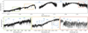 |
Fig. 1. X-shooter optical and near-infrared spectra of VHS 1256-1257 b (black). Zooms are provided in order to show the atomic and molecular absorptions that are detected in our data. |
To explore the spectral diversity of the photometric and spectroscopic observations, we used ForMoSA, a tool based on a forward-modeling approach that compares observations with grids of precomputed synthetic atmospheric models using Bayesian inference methods. This code is presented in Petrus et al. (2020) and Petrus et al. (2021), but it has been updated for this study1. The grids of synthetic spectra used as input are now provided in the standardized NetCDF4 format through the use of the xarray2 module, created and maintained by the community of meteorologists and geophysicists, which allows N-dimensional grids to be labeled, as well as parallel computations on these grids (interpolations, extrapolations, and arithmetic).
We used the grids of synthetic spectra produced by the last generation of the ATMO (Tremblin et al. 2015) models. Its specificities and the parameter space that it explores are described in Appendix C. To limit the impact of a possible bias on our estimates of the atmospheric parameters, we applied the strategy described by Petrus et al. (2020), which consists in defining different optimal wavelength ranges for different adjustments according to the specific parameter studied. Thus, to estimate the effective temperature Teff and the radius, we performed a fit between 1.10 and 2.48 μm, masking out the optical part of the spectrum that is not well reproduced by the models (panel E of Fig. 2). The lack of molecules such as CrH in the model participate in this nonreproducibility, which needs to be investigated more. The radius was estimated using the dilution factor Ck = (R/d)2, with R being the target’s radius and d the distance. To estimate the surface gravity, the metallicity, the radial velocity, and the rotational velocity, we chose to take advantage of the absorption doublet K I with the higher S/N which is sensitive to these parameters. We therefore fit our data between 1.225 and 1.275 μm, without the continuum, to avoid the contribution of the pseudo-continuum and molecular absorption to the fit. We also fit our data between 2.28 and 2.41 μm to exploit the CO overtones, which are particularly sensitive to C/O. For these last two configurations, the dilution factor Ck was calculated analytically using the relation of Cushing et al. (2008). These different fits are shown in Fig. 2. We also performed independent fits on the J, H, and K band, in addition to the LP spectrum of VHS 1256−12257 b from Miles et al. 2018. The adopted parameters from each run is given in the Table D.1.
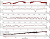 |
Fig. 2. X-shooter spectra of VHS 1256−1257 b (black) compared to the best-fit ATMO model (red). Residuals from the best fit are shown at the bottom of each panel. The fit is provided between (A) 1.10 and 2.48 μm; (B) 1.225 and 1.275 μm, a zoom around the K I doublet is shown here; (C) 2.28 and 2.41 μm, a zoom around the CO overtones is shown here; and (D) 2.90 and 4.14 μm. (E) 0.65–2.48 μm is the fit evidencing the model departure at optical wavelengths which are only shown here. |
4. Discussion
In the context of the discovery of VHS 1256−1257 b, Gauza et al. (2015) led a first empirical characterization to derive the spectral type, but also the bulk properties of the companion. Comparing the luminosity of VHS 1256−1257 b, derived from the near-infrared photometry, bolometric correction and first parallax estimate (π = 78.8 ± 6.4 mas, 12.7 ± 1.0 pc), to the predictions of the BT-SETTL evolutionary models, they derived the following physical values for the luminosity, effective temperature, surface gravity, and mass: L = −5.05 ± 0.22 dex,  K, log(g) =
  , and
, and  , respectively. Their solutions led to a rather cool atmosphere and unusually under-luminous object given its spectral type. The parallax measurement was recently revised by Dupuy et al. (2020) based on CFHT and Pan-STARRS observations placing this system at larger distances: 51.6 ± 3.0 mas (
 pc). This new estimate implies higher values for the mass (19 ± 5 MJup), surface gravity (log(g) =
  ), radius (
 RJup), and a warmer temperature (1240 ± 50 K) from the Saumon & Marley (2008) hybrid evolutionary models. It brings the absolute magnitudes of all three components in better agreement with known young objects. From a first atmospheric model analysis using near-infared spectra (NTT/SofI, 0.95–2.52 μm, Rλ = 600) and L spectra (Keck/NIRSPEC at LP band, Rλ = 1300), Miles et al. (2018) had already derived a warmer temperature of 1240 K with photospheric clouds for VHS 1256−1257 b although surface gravity and radius estimates were still affected by the early, distance determination. From their LP band spectra, Miles et al. (2018) have also reported the detection of low abundances of CH4, suggesting that nonequilibrium chemistry processes are at play between CO and CH4. The upper atmospheres of their best-fit models depart from equilibrium abundances of CH4 by factors of 10–100. Lastly, Hoch et al. (2022) estimate Teff ∼ 1200-1300 K, log(g) ∼ 3.25–3.75 dex, and C/O ∼ 0.59 with the inversion of their Keck/OSIRIS spectrum with a custom version of the model of atmosphere PHOENIX.
Our atmospheric forward-modeling analysis of the X-shooter spectra confirms the temperature of 1326 ± 2 K with ATMO models for a full fitting applied between 1.10 and 2.48 μm. Nevertheless, this estimate varies significantly with the choice of the wavelength ranges used for the fit from 1145 ± 13 K for the LP band to 1417 ± 17 K for the K band. For the surface gravity determination, we focused on the fitting of the gravity-sensitive K I lines between 1.225 and 1.275 μm. The resulting solution indicates a surface gravity of log(g) = 4.25 ± 0.20 dex, but this estimate tends to be lower (< 4.0 dex) when the fit is performed on a larger wavelength range (J, H, and K bands). Although the effective temperature and surface gravity are relatively consistent at 2σ with the evolutionary model, the radius estimate (R between 0.71 and 0.91 RJup) given by the ATMO models is not, and definitively needs to be further investigated for this family of models. At the moment, the pressure levels that are impacted by the reduced temperature gradient is assumed to be a function of the surface gravity (see Appendix C for details); an adjustment of the size of the layer impacted by the reduced temperature gradient might be needed to get a radius in better agreement with evolutionary models. We also notice that the radius estimated from the LP band is consistent with the evolutionary model, but the surface gravity is inconsistent with that obtained on the other band and too low with respect to evolutionary model predictions. This conflict between the physical properties’ estimate from models of atmosphere and from evolutionary models are well known and constitutes one of the current main challenges in the characterization of planetary atmospheres.
Finally, accessing spectral resolution up to 8100 for the K band, for which water and carbon monoxide are detected, enabled us to constrain the C/O ratio between solar and super-solar values with C/O ≥ 0.63. The metallicity appears to be solar to super-solar for all of the fits (except for the K band and H band). In the context of the cloudless ATMO models, the adiabatic index value of γ = 1.02 ± 0.01 is consistent with a decrease in the adiabatic index in the lower part of the atmospheres, as well as processes of nonequilibrium chemistry and quench CO/CH4 (i.e., they prevent the formation of CH4), as is expected for young, late L dwarfs subject to a CO/CH4 thermo-chemical instability in this scenario (Tremblin et al. 2016). Finally, we also derived the radial velocity (RV) between −4.58 and 8.77 km s−1 and the projected rotational velocities (v sin(i)) < 37 km s−1 (limited by the spectral resolution of X-shooter), compatible with the NIRSPEC data (RV =  km s−1 and
  km s−1, Bryan et al. 2018.
The [M/H] and the C/O that we measured are very similar to those measured for HR8799 b (C/O =  , Barman et al. 2015), HR8799 c (C/O =
  , Konopacky et al. 2013), and HR8799 e ([M/H] =
  and C/O =
  , Mollière et al. 2020). The solar to super-solar composition of VHS 1256−1257 b could indicate a specific atmospheric metal enrichment of solids and gas during its phases of formation and evolution if it formed within a disk by core accretion or even gravitational instability (Mollière et al. 2022). However, the existence of such a massive planet-forming disk, as well as the presence of giant planets, is not expected given the very low mass of the central binary (Burn et al. 2021). In addition, the hierarchical architecture of the whole system, a tight equal-mass binary with a planetary-mass companion orbiting at wide orbit, strongly supports a stellar-like formation by gravo-turbulent fragmentation (Padoan & Nordlund 2004). Further spectroscopic observations to directly measure of the atmospheric composition of the central binary will be important. More extended atmosphere modeling will be crucial to confirm the composition of VHS 1256−1257 b, but also its photometric temporal variability.
VHS 1256−1257 b has been identified as one of the most variable substellar objects (19.3% spectroscopic variations between 1.1 and 1.7 μm) by Bowler et al. (2020), thanks to a sequence of 11 observations (8.5 h) performed with HST. The presence of inhomogeneous cloud covers has been proposed and explored for this companion by Zhou et al. (2020), but the existence of temperature fluctuations arising in a convective atmosphere could be an alternative explanation (Tremblin et al. 2020). To explore the impact of this spectroscopic variability, we applied ForMoSA using the ATMO models on the faintest and brightest state of this spectroscopic sequence to estimate Teff and we compared them with the Teff estimated from our X-shooter data. For these fits, we calculated the dilution factor Ck analytically to avoid any possible difference in flux calibration, and we calculated the likelihood using the same wavelength range. Figure 3 illustrates the X-shooter data, over-plotted with the fits of the HST data (left panel) and the corresponding Teff posteriors (right panel). The difference in temperatures between the faintest and brightest states could be indicative of a temperature fluctuation in the atmosphere of VHS 1256−1257 b. Modulations of the temperature gradient in the region around one bar could also explain the possible CH4 variability detection observed by Bowler et al. (2020). Finally, we also note that the Teff estimate from our X-Shooter data, using the same wavelength range as the HST data (gray posterior), is coherent with the Teff estimate with the brightest state of the HST spectra.
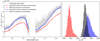 |
Fig. 3. Comparison with HST data. Left: ForMoSA fits (dash lines) of HST G141 data (solid lines). We used the maximum (blue) and minimum (red) amplitude data from the sequence of Bowler et al. (2020). We also compared these HST data with our X-shooter data. Right: comparison between Teff posteriors from the HST’s fits (red and blue) and the fit of our X-shooter data (gray). |
VHS 1256−1257 AB and b was a prime target of the JWST Early Release Science (ERS) program (Hinkley et al. 2022, PI: S. Hinkey) that acquired high-fidelity spectra with NIRSpec and MIRI at medium spectral resolution over a broad wavelength range from 1 to 28 μm (Rλ ∼ 1500–3000), respectively. The characterization of these spectra using the forward modeling approach will be treated in a future paper. This will be particularly interesting to accurately constrain the effective temperature of VHS1256 b, the abundances of important secondary gases (CO, H2O, and CH4), the importance of thermo-chemical instability, patchy cloud decks, and nonequilibrium chemistry processes at play. As proposed by Tremblin et al. (2020), the detection of direct cloud spectral signatures such as the silicate absorption feature at 10 μm, as detected for ultracool dwarfs observed with Spitzer (Suárez & Metchev 2022), will help to confirm the presence of clouds and their contribution to the spectral energy distribution and modulation of VHS 1256−1257 b. Such a signature has been detected in the spectrum provided by JWST and will be studied thoroughly in the future (Miles et al. 2022). The ERS program will serve as a benchmark for future characterization studies of young brown dwarfs and exoplanetary atmospheres.
Acknowledgments
We would like to thank the staff of ESO VLT for their support at the telescope at Paranal and La Silla, and the preparation of the observation at Garching. This publication made use of the SIMBAD and VizieR database operated at the CDS, Strasbourg, France. This work has made use of data from the European Space Agency (ESA) mission Gaia (https://www.cosmos.esa.int/gaia), processed by the Gaia Data Processing and Analysis Consortium (DPAC, https://www.cosmos.esa.int/web/gaia/dpac/consor576u tium). Funding for the DPAC has been provided by national institutions, in particular the institutions participating in the Gaia Multilateral Agreement. We acknowledge support in France from the French National Research Agency (ANR) through project grants ANR-14-CE33-0018 and ANR-20-CE31-0012. S.-P. acknowledges the support of ANID, – Millennium Science Initiative Program – NCN19_171. G-DM acknowledges the support of the DFG priority program SPP 1992 “Exploring the Diversity of Extrasolar Planets” (MA 9185/1) and from the Swiss National Science Foundation under grant 200021_204847 “PlanetsInTime”. Parts of this work have been carried out within the framework of the NCCR PlanetS supported by the Swiss National Science Foundation.
References
- Allers, K. N., & Liu, M. C. 2013, ApJ, 772, 79 [NASA ADS] [CrossRef] [Google Scholar]
- Artigau, É., Gagné, J., Faherty, J., et al. 2015, ApJ, 806, 254 [NASA ADS] [CrossRef] [Google Scholar]
- Baraffe, I., Chabrier, G., Barman, T. S., Allard, F., & Hauschildt, P. H. 2003, A&A, 402, 701 [NASA ADS] [CrossRef] [EDP Sciences] [Google Scholar]
- Barman, T. S., Konopacky, Q. M., Macintosh, B., & Marois, C. 2015, ApJ, 804, 61 [Google Scholar]
- Béjar, V. J. S., Zapatero Osorio, M. R., Pérez-Garrido, A., et al. 2008, ApJ, 673, L185 [CrossRef] [Google Scholar]
- Biller, B. A., & Bonnefoy, M. 2018, in Handbook of Exoplanets (Springer International Publishing AG), 101 [Google Scholar]
- Bonnefoy, M., Chauvin, G., Rojo, P., et al. 2010, A&A, 512, A52 [NASA ADS] [CrossRef] [EDP Sciences] [Google Scholar]
- Bonnefoy, M., Chauvin, G., Lagrange, A. M., et al. 2014, A&A, 562, A127 [NASA ADS] [CrossRef] [EDP Sciences] [Google Scholar]
- Bonnefoy, M., Zurlo, A., Baudino, J. L., et al. 2016, A&A, 587, A58 [NASA ADS] [CrossRef] [EDP Sciences] [Google Scholar]
- Bowler, B. P., Zhou, Y., Morley, C. V., et al. 2020, ApJ, 893, L30 [NASA ADS] [CrossRef] [Google Scholar]
- Bryan, M. L., Benneke, B., Knutson, H. A., Batygin, K., & Bowler, B. P. 2018, Nat. Astron., 2, 138 [Google Scholar]
- Burn, R., Schlecker, M., Mordasini, C., et al. 2021, A&A, 656, A72 [NASA ADS] [CrossRef] [EDP Sciences] [Google Scholar]
- Chauvin, G., Desidera, S., Lagrange, A. M., et al. 2017, A&A, 605, L9 [NASA ADS] [CrossRef] [EDP Sciences] [Google Scholar]
- Chilcote, J., Pueyo, L., De Rosa, R. J., et al. 2017, AJ, 153, 182 [Google Scholar]
- Cushing, M. C., Rayner, J. T., & Vacca, W. D. 2005, ApJ, 623, 1115 [Google Scholar]
- Cushing, M. C., Marley, M. S., Saumon, D., et al. 2008, ApJ, 678, 1372 [NASA ADS] [CrossRef] [Google Scholar]
- Cutri, R. M., Skrutskie, M. F., van Dyk, S., et al. 2003, VizieR Online Data Catalog: II/246 [Google Scholar]
- Dupuy, T. J., Liu, M. C., Magnier, E. A., et al. 2020, Res. Notes Am. Astron. Soc., 4, 54 [Google Scholar]
- Faherty, J. K., Riedel, A. R., Cruz, K. L., et al. 2016, ApJS, 225, 10 [Google Scholar]
- Filippazzo, J. C., Rice, E. L., Faherty, J., et al. 2015, ApJ, 810, 158 [Google Scholar]
- Freudling, W., Romaniello, M., Bramich, D. M., et al. 2013, A&A, 559, A96 [NASA ADS] [CrossRef] [EDP Sciences] [Google Scholar]
- Gauza, B., Béjar, V. J. S., Pérez-Garrido, A., et al. 2015, ApJ, 804, 96 [NASA ADS] [CrossRef] [Google Scholar]
- Hinkley, S., Carter, A. L., Ray, S., et al. 2022, PASP, 134, 095003 [CrossRef] [Google Scholar]
- Hoch, K. K. W., Konopacky, Q. M., Barman, T. S., et al. 2022, AJ, 164, 155 [NASA ADS] [CrossRef] [Google Scholar]
- Kausch, W., Noll, S., Smette, A., et al. 2015, A&A, 576, A78 [NASA ADS] [CrossRef] [EDP Sciences] [Google Scholar]
- Konopacky, Q. M., Barman, T. S., Macintosh, B. A., & Marois, C. 2013, Science, 339, 1398 [Google Scholar]
- Lucas, P. W., Roche, P. F., Allard, F., & Hauschildt, P. H. 2001, MNRAS, 326, 695 [NASA ADS] [CrossRef] [Google Scholar]
- Manjavacas, E., Apai, D., Zhou, Y., et al. 2018, AJ, 155, 11 [Google Scholar]
- Manjavacas, E., Lodieu, N., Béjar, V. J. S., et al. 2020, MNRAS, 491, 5925 [NASA ADS] [CrossRef] [Google Scholar]
- Martin, E. C., Mace, G. N., McLean, I. S., et al. 2017, ApJ, 838, 73 [NASA ADS] [CrossRef] [Google Scholar]
- Metchev, S. A., Heinze, A., Apai, D., et al. 2015, ApJ, 799, 154 [NASA ADS] [CrossRef] [Google Scholar]
- Miles, B. E., Skemer, A. J., Barman, T. S., Allers, K. N., & Stone, J. M. 2018, ApJ, 869, 18 [Google Scholar]
- Miles, B. E., Biller, B. A., Patapis, P., et al. 2022, AAS J., submitted [arXiv:2209.00620] [Google Scholar]
- Modigliani, A., Goldoni, P., Royer, F., et al. 2010, in Observatory Operations: Strategies, Processes, and Systems III, eds. D. R. Silva, A. B. Peck,&B. T. Soifer, SPIE Conf. Ser., 7737, 773728 [NASA ADS] [CrossRef] [Google Scholar]
- Mollière, P., Stolker, T., Lacour, S., et al. 2020, A&A, 640, A131 [Google Scholar]
- Mollière, P., Molyarova, T., Bitsch, B., et al. 2022, ApJ, 934, 74 [CrossRef] [Google Scholar]
- Naud, M.-E., Artigau, É., Malo, L., et al. 2014, ApJ, 787, 5 [Google Scholar]
- Padoan, P., & Nordlund, Å. 2004, ApJ, 617, 559 [NASA ADS] [CrossRef] [Google Scholar]
- Petrus, S., Bonnefoy, M., Chauvin, G., et al. 2020, A&A, 633, A124 [NASA ADS] [CrossRef] [EDP Sciences] [Google Scholar]
- Petrus, S., Bonnefoy, M., Chauvin, G., et al. 2021, A&A, 648, A59 [EDP Sciences] [Google Scholar]
- Saumon, D., & Marley, M. S. 2008, ApJ, 689, 1327 [Google Scholar]
- Skemer, A. J., Marley, M. S., Hinz, P. M., et al. 2014, ApJ, 792, 17 [Google Scholar]
- Smette, A., Sana, H., Noll, S., et al. 2015, A&A, 576, A77 [NASA ADS] [CrossRef] [EDP Sciences] [Google Scholar]
- Stone, J. M., Skemer, A. J., Kratter, K. M., et al. 2016, ApJ, 818, L12 [NASA ADS] [CrossRef] [Google Scholar]
- Suárez, G., & Metchev, S. 2022, MNRAS, 513, 5701 [CrossRef] [Google Scholar]
- Tremblin, P., Amundsen, D. S., Mourier, P., et al. 2015, ApJ, 804, L17 [CrossRef] [Google Scholar]
- Tremblin, P., Amundsen, D. S., Chabrier, G., et al. 2016, ApJ, 817, L19 [NASA ADS] [CrossRef] [Google Scholar]
- Tremblin, P., Padioleau, T., Phillips, M. W., et al. 2019, ApJ, 876, 144 [Google Scholar]
- Tremblin, P., Phillips, M. W., Emery, A., et al. 2020, A&A, 643, A23 [NASA ADS] [CrossRef] [EDP Sciences] [Google Scholar]
- Venot, O., Hébrard, E., Agúndez, M., et al. 2012, A&A, 546, A43 [NASA ADS] [CrossRef] [EDP Sciences] [Google Scholar]
- Vernet, J., Dekker, H., D’Odorico, S., et al. 2011, A&A, 536, A105 [NASA ADS] [CrossRef] [EDP Sciences] [Google Scholar]
- Zhou, Y., Bowler, B. P., Morley, C. V., et al. 2020, AJ, 160, 77 [NASA ADS] [CrossRef] [Google Scholar]
Appendix A: X-Shooter observing log
Table A.1 reports the observing conditions during our data acquirement.
Observing log
Appendix B: Empirical analysis
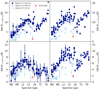 |
Fig. B.1. Equivalent widths of the detected K I lines of VHS 1256 b compared to the values of the sample of old (FLD-G) and young, low gravity (VL-G) and intermediate gravity (INT-G), brown dwarfs of Martin et al. (2017). |
The medium spectral resolution of our data allowed us to identify several strong absorption lines between 0.8 and 1.3 μm, such as neutral cesium (Cs, 0.852 μm), as well as neutral potassium (K I) doublets (1.168, 1.177 μm and 1.243, 1.254 μm). The sodium (Na I) doublet (1.138 and 1.141 μm) is also detected. These lines were not resolved in the early study of Gauza et al. (2015) given the lower spectral resolution of the GTC/OSIRIS optical and NTT/SofI nIR spectra. We therefore derived the equivalent width (EW) of the KI lines and compared them with the ones obtained by Martin et al. (2017) for a sample of old and young (low gravity and intermediate gravity) brown dwarfs as shown in Fig. B.1.
The EW of alkaline lines in the NIR has been shown to correlate with surface gravity (Cushing et al. 2005; Allers & Liu 2013; Bonnefoy et al. 2014; Manjavacas et al. 2020). The strength of these lines increases with the surface gravity due to a higher pressure in the photosphere. Therefore, they are great tracers of age. To calculate these EWs, we have exploited the resolution of X-Shooter by applying the following procedure. We constructed 100 spectra whose flux at each wavelength was randomly generated with a Gaussian law with a mean as the initial data value and a standard deviation as the data error. For each spectrum, we subtracted a Lorentzian law fitted on the line to the spectrum, which was then degraded to a resolution Rλ = 250 to accurately estimate the pseudo-continuum at the position of the line. The EW was calculated with the following:
![$$ \begin{aligned} EW\ =\ \sum _{i=1}^{n}\ \biggr [ 1 - \frac{f(\lambda _{i})}{f_{c}(\lambda _{i})} \biggl ]\Delta \lambda _{i}, \end{aligned} $$](/articles/aa/full_html/2023/02/aa44494-22/aa44494-22-eq20.gif)
with f(λi) and fc(λi) being the flux of the line and the pseudo-continuum, respectively, for each wavelength λi. Furthermore, Δλi is the wavelength step. We estimated the final EW from the mean of the series of these 100 EWs and the final error from its standard deviation.
The Figure B.1 compares the EW of each K I line calculated for VHS1256 b and the EWs calculated by Martin et al. (2017) who used the method from Allers & Liu (2013), who estimated the pseudo-continuum with a linear fit to the flux in two continuum windows defined at each side of the line (more appropriate for their data Rλ∼ 2000). For each K I line, the EW calculated for VHS1256 b is substantially weaker than the one of field and intermediate-gravity (INT-G), which confirms the VL-G classification and young age determined by Gauza et al. (2015) based on the H2OD and H-continuum spectral indices.
Appendix C: Grid description
Parameters’ space of the grid of synthetic spectra ATMO. We note that Teff is the effective temperature, log(g) is the surface gravity, [M/H] is the metallicity, C/O is the carbon-oxygen ratio, and γ is the reduced adiabatic index.
In this appendix we briefly describe the main properties of the ATMO (Tremblin et al. 2015) models and the grids that they generated and that have been used in our study (see the Table C.1). These grids are publicly available at https://opendata.erc-atmo.eu. The ATMO models assume that clouds are not needed to reproduce the shape of the SED of brown dwarfs (apart from the 10-μm silicate feature). Tremblin et al. (2016) have proposed that diabatic convective processes (Tremblin et al. 2019) induced by out-of-equilibrium chemistry of CO/CH4 and N2/NH3 can reduce the temperature gradient in the atmosphere and reproduce the reddening previously thought to occur by clouds. The grids assume a modification of the temperature gradient with an effective adiabatic index. The levels modified are in between two and 200 bar at log(g) = 5.0 and are scaled by ×10log(g) − 5 at other surface gravities. Out-of-equilirium chemistry is used with kzz = 105 cm2/s at log(g) = 5.0 and are scaled by ×102(5 − log(g)) at other surface gravities. The mixing length is assumed to be 2 scale height at 20 bar and higher pressures at log(g) = 5.0 and is scaled down by the ratio between the local pressure and the pressure at 20 bars for lower pressures. The 20 bars limit is scaled by ×10log(g) − 5 at other surface gravities. The chemistry includes 277 species and out-of-equilibrium chemistry has been performed using the model of Venot et al. (2012), and rainout is assumed to occur for species that are not included in the out-of-equilibrium model. Opacity sources include H2-H2, H2-He, H2O, CO2, CO, CH4, NH3, Na, K, Li, Rb, Cs, TiO, VO, FeH, PH3, H2S, HCN, C2H2, SO2, Fe, and H−, and the Rayleigh scattering opacities for H2, He, CO, N2, CH4, NH3, H2O, CO2, H2S, and SO2. The grids explore the following parameters: effective temperatures between 500 and 3000K (step 100K); log(g) between 2.5 and 5.5 (step 0.5); an effective adiabatic index with three values of 1.05, 1.03, and 1.01; metallicity with five values of -0.6, -0.3, 0, +0.3, and +0.6; a C/O ratio with three values of 0.3, solar, and 0.7. The last version has been used to generate a grid of synthetic spectra at medium resolution (Rλ∼10000) from 0.83 to 2.5 μm as well as lower resolution synthetic spectra (Rλ∼1000) between 0.8 and 20 μm.
Appendix D: Estimates of atmospheric and dynamic parameters
As illustrated in the Table D.1, the estimate of each parameter is strongly dependent on the wavelength range used for the fit. To take these variations into account and propose a conservative estimate of the atmospheric parameters of VHS1256 b, we followed the method described in Petrus et al. (2020):
-
The final Teff is mainly constrained by the low-resolution spectral information. It is defined by the extreme estimates from the fits that used the JHK, J, H, and K bands.
-
The final log(g) is constrained by the low-resolution spectral information, but also by the molecular and atomic absorption. It is defined by the extreme estimates from the fits that used the [1.225-1.275] μm wavelength range, as well as the JHK, J, H, and K bands.
-
Two modes seem to be observed for the metallicity, one solar (∼0.0) and one super-solar (∼0.5) mode. That is why we have chosen to leave it unconstrained by defining its final value based on the extreme estimates from all of the fits.
-
For most of the fits, the C/O converges to the upper edge of the grid. We defined its adopted values as the most conservative lower limit.
-
For most of the fits, the γ converges to the lower edge of the grid. We defined its adopted values as the most conservative upper limit.
-
Because the fit between 0.670 and 1.100 μm does not seem to reproduce the data, it has been excluded to estimate the radius. Its adopted value is based on the extreme estimates from all of the other fits.
-
The adopted value of the radial velocity is defined as the extreme estimates from all of the fits.
-
For the same reason as for the radius, we excluded the fit on the RI band to estimate the bolometric luminosity. Its adopted value is defined as the extreme estimates from all of the other fits.
Atmospheric parameters of VHS 1256-1257 b inferred from different wavelength ranges, using ForMoSA and the ATMO model grid. We use NC for "no constraint". The error bars given here are purely statistical and derived from the propagation of the small error bars of our data through the Bayesian inversion. The method used to estimate the final values is described in Appendix D.
All Tables
Parameters’ space of the grid of synthetic spectra ATMO. We note that Teff is the effective temperature, log(g) is the surface gravity, [M/H] is the metallicity, C/O is the carbon-oxygen ratio, and γ is the reduced adiabatic index.
Atmospheric parameters of VHS 1256-1257 b inferred from different wavelength ranges, using ForMoSA and the ATMO model grid. We use NC for "no constraint". The error bars given here are purely statistical and derived from the propagation of the small error bars of our data through the Bayesian inversion. The method used to estimate the final values is described in Appendix D.
All Figures
|
Fig. 1. X-shooter optical and near-infrared spectra of VHS 1256-1257 b (black). Zooms are provided in order to show the atomic and molecular absorptions that are detected in our data. |
| In the text | |
|
Fig. 2. X-shooter spectra of VHS 1256−1257 b (black) compared to the best-fit ATMO model (red). Residuals from the best fit are shown at the bottom of each panel. The fit is provided between (A) 1.10 and 2.48 μm; (B) 1.225 and 1.275 μm, a zoom around the K I doublet is shown here; (C) 2.28 and 2.41 μm, a zoom around the CO overtones is shown here; and (D) 2.90 and 4.14 μm. (E) 0.65–2.48 μm is the fit evidencing the model departure at optical wavelengths which are only shown here. |
| In the text | |
|
Fig. 3. Comparison with HST data. Left: ForMoSA fits (dash lines) of HST G141 data (solid lines). We used the maximum (blue) and minimum (red) amplitude data from the sequence of Bowler et al. (2020). We also compared these HST data with our X-shooter data. Right: comparison between Teff posteriors from the HST’s fits (red and blue) and the fit of our X-shooter data (gray). |
| In the text | |
|
Fig. B.1. Equivalent widths of the detected K I lines of VHS 1256 b compared to the values of the sample of old (FLD-G) and young, low gravity (VL-G) and intermediate gravity (INT-G), brown dwarfs of Martin et al. (2017). |
| In the text | |
Current usage metrics show cumulative count of Article Views (full-text article views including HTML views, PDF and ePub downloads, according to the available data) and Abstracts Views on Vision4Press platform.
Data correspond to usage on the plateform after 2015. The current usage metrics is available 48-96 hours after online publication and is updated daily on week days.
Initial download of the metrics may take a while.