| Issue |
A&A
Volume 670, February 2023
|
|
|---|---|---|
| Article Number | A78 | |
| Number of page(s) | 12 | |
| Section | Astronomical instrumentation | |
| DOI | https://doi.org/10.1051/0004-6361/202244421 | |
| Published online | 08 February 2023 | |
Analysis of minimum ionising particles and soft protons using XMM-Newton EPIC pn-CCD as a particle detector
1
Institute for Physics, Humboldt University of Berlin,
Newtonstrasse 15,
12489
Berlin, Germany
e-mail: vbender@physik.hu-berlin.de
2
European Space Operations Centre, European Space Agency,
Robert-Bosch-Strasse 5,
64293
Darmstadt, Germany
3
Max Planck Institute for Extraterrestrial Physics,
Giessenbachstrasse 1,
85748
Garching, Germany
Received:
5
July
2022
Accepted:
26
October
2022
Context. Spacecrafts with imaging telescopes often carry a charge-coupled device (CCD) in their focal plane to detect electromagnetic radiation. Charged particles such as electrons, protons, and heavy ions can reach the CCD and deposit their energy in the detector material. To counteract this undesirable effect, algorithms are usually implemented to reject them. On the other hand, CCDs can also be seen as particle detectors.
Aims. Even though rejection algorithms are often active to immediately discard undesired radiation, data including charged particles of ESA's XMM-Newton and Gaia were stored over the whole mission lifetime. In this article we primarily analyse and characterise the charged particles that were detected by XMM-Newton. A comparison to data from Gaia's CCDs is also presented.
Methods. To characterise the particle flux in the spacecraft orbits we used all publicly available observations where no rejection algorithm was used in combination with observations where the rejection algorithm was used. The particle flux is analysed over time and space of the XMM-Newton orbit. Comparisons to external data are shown as well.
Results. Our analysis shows that the rate of charged particle events has a modulation of about 11 yr and that particle flux and solar activity are anti-correlated. Moreover, we also show that often more than one charged particle hits the CCD simultaneously.
Conclusions. Rejection algorithms are typically used to remove charged particle detection and preserve the scientific data missions. In this article, using XMM-Newton and Gaia data, we show that by neglecting rejection algorithms, charged particles detected on CCDs can be analysed and characterised over the spacecraft orbit.
Key words: cosmic rays / Sun: activity / sunspots / methods: data analysis
© The Authors 2023
 Open Access article, published by EDP Sciences, under the terms of the Creative Commons Attribution License (https://creativecommons.org/licenses/by/4.0), which permits unrestricted use, distribution, and reproduction in any medium, provided the original work is properly cited.
This article is published in open access under the Subscribe to Open model. Subscribe to A&A to support open access publication.
1 Introduction
Space weather in the near-and far-Earth environment has negative effects on spacecraft and their scientific instruments. Onboard electronics are sensitive towards charged particles like electrons, protons, alpha-particles, and heavy ions. These particles can penetrate the spacecraft hull, trigger a single event upset (SEU), and cause deep dielectric charging or surface charging, which would cause severe damage to the spacecraft. This is just an example of possible negative effects and anomalies in spacecraft connected to charged particles (Robinson 1989; Baker 2000).
Many scientific missions carry telescopes with a charge-coupled device (CCD) in their focal plane to detect electromagnetic radiation. Charged particles entering the spacecraft can then leave characteristic tracks, as depicted in Fig. 1, by depositing a part of their energy or, at times, all of it in the detector material, much like what occurs in a semiconductor particle detector. This can change CCD properties, lead to degradation, or, if the deposited energy lies close to the energy band of the electromagnetic radiation of interest, superimpose the scientific data. For X-ray missions particles have to be very energetic in order to reach the CCD because they have to traverse the spacecraft and camera housing, which in most cases consists of an additional particle shield. The energy deposition of charged particles in the detector material through ionisation is, in most cases, large compared to that of X-ray photons. Therefore, it is rather easy to identify and reject the majority of them already on board. Nevertheless, they can affect the performance of the CCD during the specific readout cycle and have potential memory effects for subsequent cycles, as was shown by Kendziorra et al. (1999, 2000) and Meidinger et al. (1998). Minimum ionising particles (MIPs) and low-energy or ‘soft’ protons with energies between 100 keV and up to a few MeV are especially harmful to frontside illuminated CCDs as these protons can damage the sensitive structures. X-ray focusing telescopes work via grazing incidence reflections. Protons in the mentioned energy regime have similar reflection angles to X-rays and are therefore tunneled through to the CCD (Aschenbach 2007). For the NASA X-ray mission Chandra, a degradation of the front-side illuminated CCD charge transfer efficiency, and thus energy resolution, caused by soft protons was shown (Prigozhin et al. 2000; Lo & Srour 2003). For the ESA counterpart mission XMM-Newton a similar interference could be seen for the front-side illuminated European Photon Imaging Camera (EPIC) metal oxide semiconductor (MOS) instruments (Kendziorra et al. 2000), while the back-side illuminated EPIC-pn camera (Strüder et al. 2001) did not suffer from such soft-proton induced damages.
Since CCD cameras on board X-ray missions are inherently capable of operating as charged particle detectors, their observation data can be analysed. Especially regarding the described negative effects for both operational and scientific instruments, a characterisation of the detected charged particles and a detailed analysis would allow us to identify appropriate countermeasures for future space missions and to provide valuable information on the charged particle environment in the near-and far-Earth environment.
In this paper we analyse charged particles detected by the CCDs on board ESA’s XMM-Newton to seek correlations with its orbit and solar activity. XMM-Newton is well-suited to perform such an analysis. This observatory has been launched into a highly elliptical orbit of approximately 48 h, with an apogee of about 115 000 km and a perigee of ca. 6000 km (detailed numbers have changed during the mission due to orbital evolution (XMM-Newton Community Support Team 2019). Since the switch-on of the scientific payload in January 2000, it has been continuously collecting data, which also allows long-term effects to be identified. Additionally, one of its CCDs, the EPIC pn-CCD, has a comparably large pixel volume with Vpix ≈ 150 μm × 150 μm × 280 μm. It is operated in different readout modes, where for some modes, an onboard MIP rejection algorithm is activated, which identifies and discards signals above a given threshold. For details on these modes see Table 1 and Sects. 2.3 and 3.4 in Strüder et al. (2001), and Appendix A. The in-flight EPIC-pn MIP rejection algorithm is described in Freyberg et al. (2002) and in Appendix C.
Corresponding information is stored in the housekeeping data of the spacecraft and can be used for analysis. For faster modes the rejection algorithm is turned off, and it is possible to make direct use of the data. A clear record of this fact is that in these cases, the energy spectra of observations in any filter position show a distinct peak above 15 keV, which results from the Analog Digital Converter (ADC) overflow caused by charged particles, as shown for the two Small Window (SW) mode observations in Fig. 2. These properties qualify the pn-CCD for the intended purpose of analysing charged particles.
Briel et al. (2000) and Kirsch (2003) discovered that the mean MIP flux is ΦMIP ≈ 2.5 cm−2 s−1, which is more than a factor of 2 higher than the initial estimate originating from the detector simulations performed by Meidinger (2003). A survey using XMM-Newton pn-CCD data between 2000 and 2010 showed that proton flares are more likely to occur when the spacecraft moves along closed magnetic field lines (Walsh et al. 2014). However, a detailed analysis of the particle background of the XMM-Newton orbit was missing. Our work aims to bridge this gap.
In Sect. 2 we present the time dependence of the charged particle flux using EPIC-pn SW mode observations and a derived control system parameter for a similar analysis. Correlations related to the spacecraft platform and its orbit environment complement the analysis. Section 3 presents the effects of charged particles on the spacecraft platform and instruments. In Sect. 4 a comparison with the non-XMM-Newton data is discussed, and final conclusions are presented in Sect. 5.
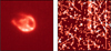 |
Fig. 1 Intensity plots, taken from an XMM-Newton EPIC-pn observation of the supernova remnant N132D located in the Large Magellanic Cloud in the 0.1–2.5 keV energy band with an integration time of T ≈ 8 h (left) and in the energy band between 15–17.915 keV with an integration time of T ≈ 10 s (right). The images were recorded on 12/02/2009 (revolution: 1681; observation ID: 0414180401; exposure ID: PNS001 in Small Window Mode). |
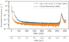 |
Fig. 2 Two XMM-Newton EPIC-pn spectra: in blue the astrophysical observation mentioned in Fig. 1; in orange the data taken with the filter wheel of the camera in closed position. The closed observation shows the intrinsic detector background mainly dominating the low-energy domain. The peak observed at higher energy is created by particle radiation entering the detector not via the telescope, but rather from all around the spacecraft. These are raw amplitude spectra (not corrected for charge-transfer efficiency) for an Open observation of N132D from 2009 (revolution: 1681; observation ID: 0414180401; exposure ID: PNS001) and a Closed observation from 2003 (revolution: 621; observation ID: 0150651101; exposure ID: PNS001 in Small Window Mode). The x-axis refers to the pulse height amplitude (PHA), which is the XMM-internal energy measure (in adu), with 1 adu ~5 eV. |
2 Charged particle analysis using EPIC-pn
There are two data sets that allow analysis of the particle flux in the area of the XMM-Newton orbit using the EPIC-pn camera. The first includes all publicly available observations where the onboard MIP rejection of particle background suppression was switched off. The second uses specially derived parameters from the mission control system that uses housekeeping data related to MIP rejection from the camera itself, called the FD131 parameter.
After the launch of XMM-Newton, it was discovered that the onboard radiation monitors were not accurately detecting all possible critical radiation for the instruments as they are not sensitive to these soft protons. In situ data of the instruments are used to calculate via the mission control system various radiation parameters that trigger the instruments to close the filter wheel in case the radiation becomes too high. One of these parameters is derived from the intrinsic MIP rejection parameter of the EPIC-pn (Kendziorra et al. 2000), the FD131 parameter (see Appendix C).
The information about the number of discarded columns from the MIP rejection algorithm is sent to ESA’s Mission Operations Centre (MOC) control system at the European Space Operations Centre (ESOC). The FD131 parameter is derived as an averaged value of discarded lines and is stored as a housekeeping parameter in the operational system and for fast data processing in an external database named MUST (Martínez-Heras et al. 2005). MUST is accessible from the ESOC network via an IDL interface. From there, we retrieved the parameter with a bin size of one minute starting in 2001 (when the FD131 parameter was introduced) until 2020.
The data were further filtered as sometimes FD131 contained values that were not taken during observations, and hence show no meaningful behaviour. The selection criteria for the file readout are summarised in Appendix E.
A concise description of all science modes of the pn-CCD including SW mode, and a description of the filter wheel positions, is given in the XMM-Newton Users Handbook (XMM-Newton Community Support Team 2019). In the remainder of this paper we refer to observations where the filter wheel is in position Open, Thin, Medium, Thick, and CalThick as ‘open’ (as soft X-rays and soft protons can reach the detector) and in position Closed and CalClosed as ‘closed’ (the 1 mm of aluminium efficiently blocks soft X-rays and soft protons).
2.1 Flux evolution over a time span of nearly 20 yr
The onboard MIP rejection algorithm is switched off for observations in small window (SW) mode of the EPIC pn-CCD. Hence, the corresponding data files qualify for a charged particle analysis. In total, 2062 pre-processed event files (dating from 18 January 2000 to 22 May 2019) for all filter wheel positions were analysed. Of these event files, 19 showed erroneous behaviour and were discarded from further calculations. They are listed in Appendix D.
Event files had to be processed from raw data (i.e. observation data files (ODFs)) by XMMSAS in a special set-up, as the default configuration removes residual MIP events in the data as if the onboard MIP rejection had already been perfectly working. Therefore, it had to be switched off in the pipeline processing software as well (see Appendix B). A similar data set of EPIC-pn SW mode observations had also been used by Bulbul et al. (2020); however, their analysis was focused on the effect of secondary particles in frames with MIP events that looked like valid X-ray events.
From the event files, we use the charge transfer efficiency (CTE) uncorrected event energies (stored in the variable PHA) because a reliable CTE correction is only available for energies below 12.5 keV, and we are also interested in analysing data above this threshold, for which there is no reliable calibration.
Inaccuracies emerge during readout and in the process that correlates the onboard time to the universal time. The influence of the time correlation uncertainty is comparably small; hence, the time accuracy is approximated to be given by the integration time for one frame. Nevertheless, respective readout parameters in SW mode are different for charged particles. Values originating from the calibration apply to photons and can be used without any further consideration only to estimate the order of magnitude of the inaccuracy, which for the time resolution is about 5.67 ms (Freyberg et al. 2005).
Low-gain observations have shown that the mean energy deposition per pixel of MIPs is approximately 50 keV (Strüder et al. 2000). Most overflow events in observational data therefore result from MIPs. The energy deposition of any relevant charged particle, except for electrons, in a directly hit pixel will lie above 50 keV. This includes soft protons mirrored by means of grazing incidence (Aschenbach 2007) during observations with open filter wheel positions, as well as alpha particles and heavy ions. These soft protons lose about 50 keV, for example, when passing through the ‘Thick’ optical light-blocking filter of EPIC. When hitting the CCD they look almost like normal valid X-ray events in terms of generated pixel pattern, and therefore cannot easily be distinguished from genuine X-rays. However, they can trigger the MIP rejection as well if they deposit the equivalent of more than 15 keV in a CCD pixel. This behaviour can be seen in observations with strong soft proton contamination as soft protons are vignetted by the telescope and the spatial distribution of rejected CCD columns also shows a vignetted pattern. Since the onboard MIP rejection algorithm for the other EPIC-pn imaging modes dismisses events and neighbouring columns with energies above 15 keV, in raw channels 3000 analog-digital units (adu), with 1 adu ~5 eV, it is very efficient in discarding charged particle events.
In our analysis, we developed a clustering algorithm to find the particle trails in the respective astrophysical data. We adopted the criterion above for our particle selection algorithm for SW observations. We selected any primary MIP and soft proton, but also secondary products such as Compton-electrons and particle showers. Figure 3 shows an example of labelling performed by the selection algorithm in frames with one, two, and three observed charged particle events. It associates connected pixels with event energies above 15 keV with a single particle event. We note that the charge carrier overflow originates from the excessive energy deposition along the tracks in Fig. 3b.
Our first approach for the SW mode data used the time frame of the readout cycle for the time-stepping. Though gaining valuable information for the subsequent analysis, we observed an undersampling of the data, and therefore turned towards the study of particle events that occurred over the duration of a full observation. To obtain a physically meaningful quantity that would be comparable for each observation, we computed respective particle rates ![${\rm{\bar \Phi }}\left[ {{\rm{c}}{{\rm{m}}^{ - 2}}{{\rm{s}}^{ - 1}}} \right]$](/articles/aa/full_html/2023/02/aa44421-22/aa44421-22-eq1.png) defined as
defined as
 (1)
(1)
where  is the mean number of charged particle events per frame, FTSW = 5.67 ms the frame time, and ASW the sensitive area of the CCD. The statistical uncertainties can be estimated as usual from the standard error of the mean. Figure 4 plots the values over the whole mission lifetime. Using all applicable SW mode data, we observe a modulation of about 11 years, where the lower bound varies between 2 and 4.5 cm−2 s−1. At times we can see high deviations from the lower bound.
For the housekeeping parameter FD131, we first consider the distribution of values in one example. Figure 5 shows the normalised frequencies of FD131 values in a full frame (FF) mode observation on 12 March 2001. We can see the outlines of a Gaussian-shaped peak between the values 100 and 150, and a tail for values greater than 150. Time-resolved measurements show that both features are constantly present. This suggests a minimum of two components of charged particles that contributed during the observation.
To study the overall behaviour of the FD131 count in all available modes, i.e. extended full frame(eFF), FF and large window (LW) mode, over the full mission, we calculated expectation values over all observations. Additionally, to analyse the FD131 distributions, we also considered respective standard deviations. The referring values are plotted in Fig. 6. The expectation values show in all modes the same large-scale behaviour, namely an 11-yr modulation. This coincides with what we highlighted in the previous section (see Fig. 4). Thus, the periodic fluctuation of the charged particle flux has been shown in two separate ways: directly, over the number of charged particle events and indirectly, over the derived parameter FD131, which represents a lower bound to the number of charged particle events. The different offset values for the various modes in Fig. 6 originate from different normalisation factors that are connected to the mode area, and the calculation procedure of the parameter1. We note that the gap in 2011 arises from an error that occurred during the parameter retrieval from the MUST archive, where no values were written to the file.
The standard deviations are large with respect to the expectation values, which emphasises our guess from Fig. 5 that the upper tail results from randomly occurring events with bursts of charged particles. To estimate the time dependence of the component connected to the Gaussian-shaped peak, integrated counts over singles months have been calculated, and a Gaussian fit curve was applied to the data in FF mode. Figure 7 shows a typical plot for May 2003. We observe the same characteristics as in Fig. 5, but now the features in the curve are smoothed out.
We can use the fit parameters and in particular, the mean values and standard deviations to analyse the progression flux of the seemingly constant charged particle component over time. Figure 8 shows all calculated mean values and standard deviations over the full mission. The above-mentioned modulation effect is even more visible in this plot. The progression is smoothed out, and it is possible to identify detailed features. This supports our overall assumption that the peaks in Figs. 5 and 7 result from equal particle components.
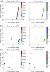 |
Fig. 3 Demonstration of the clustering algorithm for distinguishing (a) one, (b) two, and (c) three particle tracks in a single readout cycle in SW mode. Energy values below 3000 adu are assigned cluster number 0. Pixels have a size of 150 × 150 μm2 and SW mode covers an area of 63 × 64 pixels. |
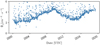 |
Fig. 4 Rates of charged particle events averaged over individual small window mode observations for the whole mission lifetime until 2020. A modulation of about 11 yr can be seen. |
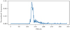 |
Fig. 5 Normalised frequencies of FD131 values that occurred during a full frame mode observation on 12 March 2001 (observation ID: 0086360301). The outlines of at least two particle components can be identified. They can be characterised by a Gaussian-shaped peak and a tail at high rates. |
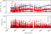 |
Fig. 6 Expectation values of the FD131 parameters (top) and respective standard deviations (bottom) calculated over signal observations in eFF, FF, and LW camera modes. The different offsets are caused by individual mode normalisation of the parameter. The same 11-yr modulation as in the prior analysis can be seen. The gap for 2011 results from a readout error that occurred during the data retrieval from the MUST archive. One data point represents one observation. |
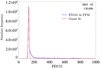 |
Fig. 7 Integrated frequencies of FD131 parameter values (blue line) for May 2003 in FF mode. To estimate the parameter position generated by the charged particle component referring to the Gaussian-shaped peak, a Gaussian function was fitted to the data (red line). The peak position of the fit was later used to estimate the averaged monthly value of FD131. |
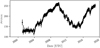 |
Fig. 8 Expectation values μFD131 with standard deviations (as error bars) from Gaussian fits for monthly integrated FD131 values in FF mode. The curve shows a smoothly outlined 11-year modulation without the occurrence of local peaks. |
2.2 Correlations to Earth distances
Orbit parameters can be obtained for any point in time of the mission. We are therefore not restricted to charged particle parameters for SW mode but can also use FD131 data sets for eFF, FF, and LW modes to look for possible dependences to the orbit. The distance of the spacecraft to Earth poses a promising orbit parameter for closer analysis. It can be derived directly from the spacecraft’s state vector through the calculation of the euclidean norm.
To look for a possible dependence of the charged particle flux with respect to the spacecraft’s distance to Earth, we consider the FD131 count rates defined in Eq. (2), which we already calculated for the LCL trip correlation analysis in the previous section. The following steps were performed for all available camera modes and integration times and lead to similar results. As an example, we consider all calculated rates with an integration time of T = 60 s and increment time Δt = 60 s in eFF mode. We calculated the distance to Earth for every time step and store the resulting tuples in an array. From this array we derived a two-dimensional histogram with an increment for the distance to Earth of about 1400 km and an increment for the FD131 rate of about 0.05 s−1. Since it is not ensured that within every distance interval we have the same total number of data points, we needed to find a normalisation that leads to statistically comparable values. We considered data points within equal distance intervals and different FD131 rate intervals as separate one-dimensional histograms and normalised the bins such that their values would equal the respective probability density function.
From this procedure we obtained the plot depicted in Fig. 9. The colour scale refers to the calculated probability density values, which are normalised to an integral value equal to one along each column. According to Fig. 9, the majority of data points lie within an interval of about 5 to 10 s−1. For distances larger than 80 000 km, we observe a fine structure for global maximum probability values, which fades out gradually as we go to smaller distances. Probabilities for rates above 10 s−1 become significant below 65 000 km, which leads to an overall flattening of the distributions in this regime. At very short distances, we can see an apparent undersampling of the histograms. To highlight the increase in data points with high count rates at close spacecraft distances, we reassign the colour mapping and set probability values above 0.2 equal to zero. This plot is shown in Fig. 10. As we can see, an increase in data points with count rates above 10 s−1 can be observed already at 80 000 km from Earth. From this point, it rises gradually with increasing probabilities at higher count rates as we go to closer distances.
By using data from SW observations, we can make an additional comparison between observations that were performed in open and in closed filter wheel position. We considered the SW charged particle event rates from Sect. 3.2 with an integration time of T = 60 s and an increment time of Δt = 60 s. Rates of each time step are plotted against their respective distances for open in Fig. 11 (top) and for closed in Fig. 12 (top).
For values that were taken during open observations, we find an increasing number of high count rates as we go towards smaller distances to Earth. In Fig. 11 (bottom) we plot the distribution of the respective column-wise probability distributions, as derived before. These reflect our observations for the FD131 count rates that low rates are more likely to be found at large distances. On the other hand, high rates do not simply occur as single values, but pose a true statistical weight when the spacecraft is close to Earth.
The corresponding plots for closed observations show a different picture. Data points are almost equally distributed within a band of 2–4 s−1. Though we observe the highest count rates at distances between 50 000 and 60 000 km, we can see from the probability distributions that these values have little weight, and therefore they could also result simply from higher statistics.
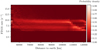 |
Fig. 9 Distributions of probability density functions along each column for given spacecraft distances to Earth with a bin width of 1400 km are plotted with respect to FD131 rates in FF mode with a bin width of 0.05 s−1 that were calculated for the full mission. At large distances the outlines of a fine structure are visible, and at close distances the probability of finding high count rates rises. |
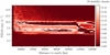 |
Fig. 10 Distributions of probability density functions along each column for given spacecraft distances to Earth with a bin width of 1400 km are plotted with respect to FD131 rates in FF mode with a bin width of 0.05 s−1 that were calculated for the full mission. Probability values above 0.2 are cut off and set to zero. A rescaling of the colour map highlights the effect of increasing probabilities for high count rates at small distances. |
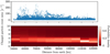 |
Fig. 11 Point clouds of calculated actual charged particle event rates (top) and referring to probability distributions with a bin width of 0.1 s−1 (bottom) with respect to the spacecraft’s distance to Earth with a bin width of 7664 km for open SW mode observations. |
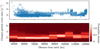 |
Fig. 12 Point clouds of calculated actual charged particle event rates (top) and referring to probability distributions with a bin width of 0.1 s−1 (bottom) with respect to the spacecraft’s distance to Earth with a bin width of 7816 km depicted for closed SW mode observations. |
2.3 Correlations to spacecraft attitude
The spacecraft’s reference frame has been coaligned with the basis vectors of the J2000 equatorial coordinate system. Thanks to ESOC flight dynamics, the spacecraft attitude was obtained for all eFF, FF, LW, and SW mode observations. Figure 13 shows the calculated directions for all SW pointing observations in right ascension and declination. Prominent features such as the Large and Small Magellanic Clouds (LMC and SMC) and the inner Galactic plane (GP) are clearly visible.
A detailed discussion on attitude determination with quaternions can be found in Chap. 12 of Wertz (1978). We can use this data to investigate whether there are preferred directions or areas in the sky for charged particle events. Figure 14 shows directions of FF observations; the colour-coding is proportional to the mean FD131 value during a given observation. We see several occurrences of peak values, equally distributed over the equatorial coordinates, but no apparent clusters. To treat problems connected to undersampling and to obtain a better areal statement, the full plane can be divided into quadrants, which we choose to be of 30° × 30°. We calculate the mean integral values from observations that are contained within each quadrant. The plot is given in Fig. 15. We find areas of increased integral value in the upper parts of the plane at declination between 30° and 90° with a maximum value for right ascension between 240° and 300°. The lower parts of the sky also show lower values.
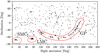 |
Fig. 13 XMM-Newton attitude for SW mode pointing observations in right ascension and declination. Prominent features such as the SMC, LMC, and the inner GP are emphasised by red dashed lines. |
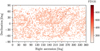 |
Fig. 14 XMM-Newton attitude map for pointing observations in FF mode given in right ascension and declination. The colour-coding is proportional to mean FD 131 values. |
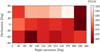 |
Fig. 15 Averaged FD131 values from FF mode observations within windows of 30° × 30°. The upper part of the sky shows slightly elevated values. |
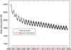 |
Fig. 16 Power generated from the XMM-Newton solar arrays. The sinusoidal variation is a seasonal effect where more power is generated in winter since the spacecraft is closer to the Sun. The red line shows the peak power consumption. The power margin in 2022 is of the order of 450 W. |
3 Effects of charged particles on the spacecraft platform and instruments
Particles approaching the spacecraft and its instruments can have various effects on their performance and lifetime. Over the 20 yr of operating XMM-Newton in orbit, we see minor degradation effects on silicon devices like the instrument’s CCDs (Kirsch et al. 2005) and the solar panels that generate the energy for the spacecraft (Kirsch et al. 2014). In addition, so-called single event upsets (SEUs) created by a high-energy particle can upset the onboard software and the subcomponents of the spacecraft as well, especially the latching current limiters (LCLs). These are electronic switches with current limiting properties; in other words, if the switch is closed and the current flowing through it is higher than the specified limit, the switch will open automatically. LCLs are used to connect all electrical consumers to the main bus, and through their current limiting property they ensure that a possible broken consumer is not damaging its surrounding by draining too much current or causing a main bus under-voltage.
3.1 Solar array degradation
XMM-Newton has two fixed solar array wings, with three sections each. At the beginning of the mission in 1999 they generated a power of approx 2400 watt, which has degraded over time due to radiation effects (see Fig. 16). The consumption is between 450 and 1300 watt driven mainly by the mirror heaters. The power production shows a sinusoidal variation, which is a seasonal effect where more power is generated in winter since the spacecraft is closer to the Sun.
3.2 LCL trips
A LCL can switch from on to off, or the other way around, without any direct command; this is referred to as a LCL trip.
LCL trips can lead to complications for the spacecraft, potentially endangering it, for example if a reaction wheel’s electronics or an important heater is switched off. This is mostly counteracted by automated software on board or on the ground, but a combination of this effect with a ground station outage or other complications on board is still a critical moment for the spacecraft in terms of attitude and orbit control or thermal control. Although it is a well-known phenomenon that also affects other spacecraft, why they occur is still unclear; knowing their causes would facilitate spacecraft operations. We investigated the possibility that LCL trips are correlated to charged particles. We looked at 56 trips that occurred from the start of the mission of XMM-Newton until 30 October 2019. The LCL history data are kept by the mission operations team on a dedicated website. As measures of particle flux, we used the number of charged particle events that we calculated for SW mode and the FD131 parameter that is available for EPIC-pn eFF, FF, and LW modes. Correlations can be established only for LCL trips that occurred while the camera was in one of these modes. Out of 56 registered trips considered, there were two occurrences during eFF, 21 during FF, one during LW, and five during SW mode observations. All others occurred during either Timing or Burst modes or inside the radiation belts while the camera was not operational.
If LCL trips are caused by electric charging effects such as deep dielectric charging or surface charging, we should be able to see a correlation to either charged particle rates or the integrated amount of deposited charge. For the ith increment step in the jth observation, rates Rij and integrated count Iij are defined as
 (2)
(2)
 (3)
(3)
where T is the integration time, Δt the increment time, and nj (tk) the number of charged particle events or the FD131 value in the kth frame at time tk of the jth observation. For our calculation an increment time of Δt = 60 s and an integration time of T ∈ {60 s, 600 s, 3600 s} was chosen and applied to the respective data sets in SW, eFF, FF, and LW. For all modes and integration times the same results were obtained. Therefore, we consider as an example the integrated count of FD131 values in FF mode with an integration time of T = 3600 s. Figure 17 shows the averaged values over each observation and values of increment steps during which LCL trips occurred. We can see that only one trip occurred during a high integration count. This does not necessarily mean that these two parameters are independent since the population of high integration counts is small compared to that of lower integration counts. We calculated the histogram over all increment steps to obtain a statistically meaningful test and normalised to a probability density function.
A plot of the function is shown in Fig. 18. In addition, we marked the integrated count values that were recorded while LCL trips occurred. We note that the plot includes only values up to 20000, and therefore cuts off one of the LCL values depicted in Fig. 17. For an even distribution, we would expect to see, in the case of correlation, marks for LCL trips with increasing density as the integrated count rises. Here we find several peaks that originate from the outlines of the lower boundary in Fig. 17, and therefore, as we show in the previous section, from the solar cycle. In the case of correlation, marks for LCL trips would be clustered around the peaks and occur with increasing density as the integrated count rises. We can identify several clusters, but none of them coincides with local peaks. Equal results were obtained for different integration times and also when replacing the integrated count by rates. Therefore, no statistical correlation can be substantiated between measures of charged particle flux as we have derived them and the occurrence of LCL trips.
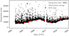 |
Fig. 17 Averaged FD131 values Ij over each observation in FF mode with an integration time of T = 3600 s (black dots) and respective values that were observed during times where LCL trips occurred (red crosses). |
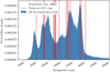 |
Fig. 18 Probability density for the occurrence of integrated FD131 values during an increment step with integration time T = 3600 s for the whole mission. Red lines indicate values that were recorded during LCL trips. In the case of parameter dependence the red lines would be clustered around peak probability values. |
4 Comparison with non-XMM-Newton data
In the remainder of this paper we compare the detections using XMM-Newton CCDs with other external data, such as sunspot number (SSN) and the data from another ESA mission, Gaia. From its observing position near the second Sun-Earth Lagrange point (L2) the Gaia focal plane is able to measure the galactic cosmic ray and solar energetic particle flux at a distance of 1 AU from the Sun. The Gaia orbit around L2 is large enough that there is little or no effect from the Earth’s magnetic field on the measured flux.
4.1 Comparison between sunspot number and XMM-Newton EPIC-pn
There is a known solar-cycle modulation of the Galactic cosmic ray (GCR) component (Gleeson & Axford 1968). If charged particle events from XMM-Newton, as described in Sects. 2 and 2.1, result from GCR particles, it should be possible to experimentally substantiate a correlation to the solar-cycle modulation.
In order to obtain a measure of solar activity, data for the sunspot number was retrieved from the SILSO website (WDC-SILSO, Royal Observatory of Belgium, Brussels 2020). In these files, the daily values Nd were calculated from the formula
 (4)
(4)
where Ns is the number of sunspots and Ng the number of groups counted over the entire disc. Daily error values result from the respective standard deviation
 (5)
(5)
of raw numbers  provided by all n stations. The standard error
  of Nd can be estimated as usual via
 (6)
(6)
The respective information is provided in the data files.
Furthermore, monthly and yearly values Nm,y are provided as simple arithmetic means of the daily total sunspot number over all days of each calendar month and year. The standard deviation can be computed from the weighted mean of daily standard deviations via
 (7)
(7)
and the standard error  can be estimated again in analogy to Eq. (6).
Figure 19 summarises the mean charged particle event rates per SW mode observation, the mean sunspot number per day and month, and the expectation values for the FD131 parameter resulting from a Gaussian fit of the respective peak within the spectrum (see Sect. 2.1).
As we can see, the measures of particle flux and solar activity are in anti-phase. It is likely that solar activity drives two concurrent effects. On the one hand, it suppresses the GCR component that reaches the spacecraft with increasing solar activity. On the other hand, additional particles that are generated through solar flares could potentially reach XMM-Newton and cause additional charged particle events through secondary particle showers or directly as soft protons. Since the FD131-related values in Fig. 19 presumably only include particles that originate from the GCR component (in particular for closed observations), they are suitable to be compared to monthly averaged sunspot number values between 2001 (when the FD131 parameter was introduced) and 2020. The charged particle rates, on the other hand, include all types of events, and will therefore show local peaks if solar flares contribute directly to the charged particle background. Hence, we compare this data to the sunspot number that was observed during that day between 2000 (when the scientific payload was switched on) and 2020. Figure 20 plots the respective measures against each other. Both point clouds show an anti-correlating behaviour of the measure of charged particle flux to the number of sunspots. To quantify the anti-correlations, we can calculate the respective covariance matrices and correlation coefficients as in the previous section. The estimators for the two cases result in
 (8)
(8)
 (9)
(9)
where ρCP represents the correlation coefficient for the comparison to the charged particle event rates and ρFD131 to FD131 values. The result for ρFD131 indicates a clear anti-correlation. Furthermore, we note that peak values in the mean charged particle rates (see Fig. 20, top) do not occur for large numbers of sunspots, but are rather randomly scattered. The value for ρCP also indicates an anti-correlation, though the effect is not as pronounced as for the FD131 case, which implies that the observed local peaks are uncorrelated to the sunspot number. This hypothesis can be further substantiated if we reevaluate ρCP, taking into account only values below 5 cm−2 s−1. Then we find ρCP = −0.66. It is therefore unlikely that the solar activity contributes directly to the number of observed charged particle events. SRG/eROSITA at L2 found a weak correlation of a few per cent in the 27-day modulation of the MIP rates, which was assigned to solar rotation and the indirect effect of GCR shielding (Freyberg et al. 2020). Even so, this does not include an indirect influence through trapped radiation, as shown by Walsh et al. (2014). A similar correlation of rejected background events with the solar cycle has recently been presented by Grant et al. (2022) in a long-term analysis of Chandra ACIS and Alpha Magnetic Spectrometer (AMS) data. The relation of cosmic ray modulation and solar cycle activity variations has been found and analysed in various studies (e.g. Shen & Qin 2018), also at Mars and beyond using Mars Express and Rosetta (e.g. Knutsen et al. 2021).
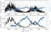 |
Fig. 19 Comparison between solar activity and the flux of charged particles as observed by XMM-Newton. Top: mean charged particle events rate |


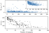 |
Fig. 20 Mean charged particle event rates |

4.2 Comparison between Gaia and XMM-Newton EPIC-pn
Gaia has a billion pixel focal plane. As presented by Gaia Collaboration (2023) the data quantities potentially generated by this system are much too large to be either stored on board or sent to the ground in their raw format. For this reason Gaia is performing real-time analysis of the acquired data in order to identify the stellar point source objects that are of interest to the mission. The first stage of this object identification process is performed on the data acquired by the 14 CCDs dedicated as ‘sky mapper’. In addition to the signals from stellar point sources there are other potential causes of more or less pointlike signals, one of which is ionising particle tracks referred to as prompt particle events (PPEs). The important difference between stellar sources and ionising particles is that the optical sources are focused by the optics of the telescope, while the ionising particles are not. Onboard differentiation between these signals is therefore based on their point spread functions (PSF). Although the PPE signals are considered to be noise and are rejected from further processing on board, the accumulated number of detected PPEs is routinely transmitted to the ground for each of the 14 sky-mapper CCDs allowing a Gaia PPE rate to be calculated.
Gaia imaging CCDs are operated in time-delayed integration mode where the pixel lines are read out at a constant rate. There is a concept of a gate in the Gaia CCDs, which is normally used in the presence of bright sources to prevent saturation of the images of these sources. When activated, all signal integrated before the pixel line with the gate is flushed so that the images are integrated over a shorter distance and there is consequently a reduced integration time. In each CCD there are a number of gates that can be activated depending on the brightness of the source being imaged, where the selection of which gate to activate is made in real time by the onboard video-processing units. The sky-mapper CCDs are a little different because they are located at the edge of the Gaia telescope fields of view. They are operated with the gate number 12 permanently activated in order to exclude the possibility of optically distorted signals from the periphery of the field of view being imaged. Operation of the sky-mappers in this way reduces the number of pixel lines that are integrated to 2900, reducing the effective area to 17.1 cm2 and the integration time to 2.85 s. The Gaia focal plane is located inside the payload module where the surrounding spacecraft structure provides some high-pass energy filtering of the ionising particle flux. The protection is equivalent to a few millimetres of aluminium shielding, which is sufficient to stop most of the solar wind particles from a quiescent Sun, but is largely transparent to the majority of galactic cosmic rays. During periods of high solar activity the energy of solar energetic particles is often increased above the shielding threshold, causing these events to be visible in the PPE data. As the spacecraft rotates, any PPE signal from the Sun may vary with a six-hour signal due to a combination of two effects. Firstly, the orientation of the focal plane to the Sun changes the area exposed to the solar flux and secondly, the spacecraft structure is not isotropically arranged around the focal plane, which results in a varying thickness of shielding between the focal plane and the Sun (de Bruijne et al. 2015).
To compare modulation effects in the particle count rates between Gaia at Lagrange point 2 (L2) and XMM-Newton with its highly eccentric orbit, we sampled the data set to calendar months. We further computed the according fluxes using the sampling time and effective detection area AGaia = 17.1 cm2 and normalised the FF mode FD131 parameter values (see Sect. 2.1) and the Gaia data set to their values from December 2018. Both curves in Fig. 21 show the same large-scale modulations, which suggests that the leading contributions to the particle background are the same for both spacecraft. Exceptional points for the particle rates can be observed in September 2017, June 2015, and September 2014 for Gaia. These are related to solar energetic particle (SEP) events (see e.g. Cohen & Mewalt 2019 and references therein). XMM-Newton did not observe these events as the FD131 parameter was not recorded during these periods since the EPIC-pn camera was not actively observing due to high-radiation safety requirements. When comparing the sunspot numbers over the whole period, we note again an anti-correlation to solar activity (Fig. 22). Figure 22 depicts the mean flux values for XMM-Newton per observation in all filter modes and the respective derived averages per calendar month. Again, the exceptionally high values for Gaia in September 2017 are not captured by XMM-Newton for the reasons mentioned above.
Furthermore, we observe a constant mean offset between XMM-Newton EPIC-pn SW mode charged particle fluxes (see Sect. 2) and Gaia of 0.3 cm−2 s−1 with a standard deviation of 0.2 cm−2 s−1, if we do not take into account data points for the previously mentioned three exceptionally high particle rates. This offset could be due to uncertainties in the Gaia sensitivity for particle events but it could also reflect a real difference due to different orbital locations.
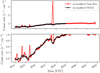 |
Fig. 21 Comparison between monthly averaged particle count rates measured by Gaia and FF mode FD131 values for XMM-Newton. Measures were normalised to their respective values on December 2018. Both curves show the same overall behaviour (top). Exceptional points can be observed in September 2017, June 2015, and September 2014 (bottom), which are related to SEP events (Cohen & Mewalt 2019). |
5 Discussion and conclusions
For the determined measures of charged particle flux (i.e. the FD131 parameter values and the number of charged particle events in SW mode) we find an 11-year modulation of the data (see Figs. 4 and 6).
From the analysis on FD131 values in Sect. 2.1 we identified at least two components in its behaviour over time (see Fig. 5):
a first component shows a particle flux that stays at a constant value over a period of approximately one month. The frequencies of the respective count rates appear in the shape of a Gaussian distribution and are the sole contribution to closed SW mode observations;
a second component contributes an irregular flux of particles and leads to a tail at high count rates.
Plotting expectation values of Gaussian fit curves (Fig. 7) to the first particle component over time results in a smooth curve with an 11-yr modulation (Fig. 8) that shows no occurrences of local high peak values. As a result, we believe that this first particle component consists primarily of MIPs that underlie the actual 11-yr modulation. The respective particle flux has an expected lower threshold that varies approximately between 2 counts cm−2 s−1 and 4.5 counts cm−2 s−1 and is given by the outlines in Fig. 4. These values represent a lower limit and have an upper inaccuracy of the order of 29% given by the detector lifetime. This result stands in agreement with the factor of 2 discrepancy between early observations and detector simulations reported by Kirsch (2003) and Briel et al. (2000).
Furthermore, in Sect. 4.1 we observed that the MIP component is anti-correlated with the sunspot number, and thus to solar activity. This observation confirms the expectation described by Gleeson & Axford (1968), thus indicating that MIPs detected by the pn-CCD originate from the GCR component. A further observation on this particle component is the apparent fine structure of the particle flux, which we observed during the LCL and distance to Earth analysis depicted in Figs. 17 and 9.
Since the second component is observed for open observations only, we can assume that it consists of large parts of soft protons that enter the spacecraft by means of grazing incidence (Aschenbach 2007). Again, it is likely that secondary particles from particle showers make a significant contribution.
We observed a dependence of the second particle flux component on the spacecraft’s distance to Earth (Fig. 11). The probability rises for higher particle bursts as the satellite draws closer and is also significant outside the Van Allen belts. Furthermore, no direct correlation could be established between the second component and the number of sunspots (i.e. high values for the number of charged particle events do not correlate directly with high solar activity).
In addition, we showed that LCL trips have no statistical dependence on measures of charged particle count rates or on measures of accumulated charge. Lastly, the analysis of dependences of the charged particle flux measures with respect to the attitude showed no clusters of observations with high rates. Nevertheless, mean values over areas in the sky revealed that areas with an inclination between 30° and 90° and in particular with a right ascension between 240° and 300° show elevated flux values for multiple different measures (Fig. 14).
When comparing XMM-Newton data to Gaia, we find a similar large timescale behaviour. This suggests that the particle background for both detectors is composed of the same components. The constant offset of (0.3 ± 0.2) cm−2 s−1 may both be detector and orbit dependant.
We speculate that the offset that we see between the predicted MIP values and the measured MIP values is due to the fact that primary MIPs generate secondary particles in the camera housing, which mimic a higher number of MIPs actually detected by the CCD. This, however, cannot be deconvolved by our analysis. In future studies it might be feasible to substantiate this difference via ground measurements and simulations. Possible expansions to this work can be the following:
performing computations to include the simultaneous correlation of attitude, orbit, and the number of charged particle events, to test for geomagnetic particle flares as observed by Walsh et al. (2014);
combining information on the orbit and the position of the Sun (which still needs to be obtained) to estimate particle fluxes at spacecraft positions that are close to the magnetotail of the Earth. These computations would be valuable for satellites at L2, such as eROSITA, and in the future for Athena;
separating the two mentioned particle flux components, as discussed above, for open observations, and therefore to study MIPs and soft protons separately. To acquire the respective separation, one would need to calculate histograms for the number of charged particle events over longer timescales at integration times much bigger than the frame time (e.g. 60 s). This would provide similar plots to those acquired for the FD131 parameter in Sect. 2.1. The position of the respective peak assigned to the first component could then be used as a criterion to choose between the first and second component frames retrospectively.
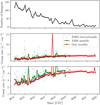 |
Fig. 22 Comparison between solar activity and charged particle rates as observed by XMM-Newton and Gaia. Top: monthly averaged sunspot number; middle: particle count rates measured by Gaia (red), average particle count rates per month (green), and observation measured by XMM-Newton (black); bottom: zoom-in on the low-level region of the middle panel (see Sect. 2). |
Acknowledgements
We would like to acknowledge the support from the ESOC XMM-Newton Flight Control and Flight Dynamics Team, especially D. Webert, A. McDonald, and C. Dietze and the MPE technical support (in particular H. Baumgartner) for providing the computational resources needed for the analyses. We also thank E. Serpell from the Gaia Flight Control team for the discussions and his support.
Appendix A EPIC-pn instrument submodes
The EPIC-pn camera can be operated in six different scientific submodes, depending on the scientific needs, such as pile-up limit or time resolution. Table A.1 lists the relevant information in the context of high-energy particles and their suppression. For more details, see Strüder et al. (2001).
EPIC-pn submodes and relevant parameters for particle background: status of onboard MIP rejection, number of active CCDs, the frame time in [ms], and the approximate accumulation time of the MIP rejection counters (20 frame times) in [s].
Appendix B Non-standard XMMSAS parameter settings
The EPIC-pn onboard MIP rejection sometimes works incompletely for the 12-CCD modes, and is switched off for the 1-CCD modes. The remaining MIPs in the data are removed completely with default set-up parameters on the ground using the standard XMMSAS pipeline tasks (in particular in epframes). To enable the analysis of the remaining MIPs, one has to choose non-standard parameter settings (without change to the programs otherwise), which we document in the following for reproducibility:
epchain runscreen=N screenlowthresh=0
	runbadpixfind=N getnewbadpix=N
	anmip=4095 anmaxmip=4095.
This does not screen invalid (non-X-ray) events, does not apply a low-energy filtering, does not perform a bad pixel search, sets the MIP trigger threshold to the maximum channel number 4095 (being equivalent to switching it off), and also disables the flagging of complete frames as contaminated by a large number of MIP events.
Appendix C Derivation of FD131 parameter from EPIC-pn housekeeping values
For a detailed description of the XMM-Newton EPIC-pn inflight MIP rejection algorithm, see Freyberg et al. (2002). The main parameters are the trigger threshold anmip (default 3000 adu, with 1 adu being about 5 eV this corresponds to about 15 keV for the charge in a single pixel) and the number of columns that are rejected in this CCD to either side in addition to the CCD column containing a trigger pixel in this readout cycle (default 1). Moreover, if more than anmaxmip (default 63) pixels above the MIP trigger threshold in a single readout frame of a CCD are found, then the whole frame gets rejected, no matter whether they are due to a complete CCD row or column being above the limit. The number of rejected columns DSLIN per time unit (default 20 readout cycles) is recorded and transmitted via science and camera housekeeping stream.
FD131 is the average of the averages of the four individual quadrant DSLIN values, Ax_DSLIN (x=0,1,2,3). The values are read from the main periodic housekeeping files (PNX00000PMH) from parameters F1330, F1375, F1420, F1465, respectively. The averages are taken over 16 data values, with a sampling cadence of 8s this gives an integration interval of 48s. ‘F’ stands for EPIC-pn housekeeping, ‘D’ for derived parameter, and ‘131’ is the 131st such defined parameter.
Appendix D Discarded Small Window mode event files
List of discarded SW mode event files
Appendix E Criteria for the FD131 file readout
For the FD131 file readout several criteria had to be applied to make the data processable for further analysis:
The data files contain FD131 values also for modes that cannot be identified as observations such as ‘IDLE’, ‘OFF-SET_NOISE’, and ‘SAFE_STDBY’. Only values that were flagged with
‘EXT_FULL_FRAME’,
‘FULL_FRAME’, or
‘LARGE_WINDOW’
In addition the data was filtered for obvious artefacts such as character strings with ‘*******’ instead of a numeric value.
References
- Aschenbach, B. 2007, Proc. SPIE, 6688, 157 [NASA ADS] [Google Scholar]
- Baker, D. 2000, IEEE Trans. Plasma Sci., 28, 2007 [CrossRef] [Google Scholar]
- Briel, U. G., Aschenbach, B., Balasini, M., et al. 2000, SPIE, 4012, 154 [NASA ADS] [Google Scholar]
- Bulbul, E., Kraft, R., Nulsen, P., et al. 2020, ApJ, 891, 13 [Google Scholar]
- Cohen, C., & Mewalt, R. A. 2019, in Solar Heliospheric and INterplanetary Environment (SHINE 2019), 140 [Google Scholar]
- de Bruijne, J. H. J., Allen, M., Azaz, S., et al. 2015, A&A, 576, A74 [NASA ADS] [CrossRef] [EDP Sciences] [Google Scholar]
- Freyberg, M. J., Briel, U. G., Dennerl, K., et al. 2002, The XMM-Newton EPIC-pn camera: spectral and temporal properties of the internal background, Technical report, available at https://xininweb.esac.esa.int/docs/documents/CAL-TN-0067-0-0.pdf [Google Scholar]
- Freyberg, M. J., Burkert, W., Hartner, G., Kirsch, M. G. F., & Kendziorra, E. 2005, Comparison of EPIC-pn ground-based and in-orbit calibration measurements, Technical report, available at https://xmmweb.esac.esa.int/docs/documents/CAL-TN-0081.pdf [Google Scholar]
- Freyberg, M., Perinati, E., Pacaud, F., et al. 2020, SPIE Conf. Ser., 11444, 114441O [Google Scholar]
- Gaia Collaboration (Vallenari, A., et al.) 2023, A&A, in press, https://doi.org/10.1051/0004-6361/202243940 [Google Scholar]
- Gleeson, L., & Axford, W. I. 1968, ApJ, 154, 1011 [NASA ADS] [CrossRef] [Google Scholar]
- Grant, C. E., Miller, E. D., Bautz, M. W., et al. 2022, SPIE, 12181, 121812E [NASA ADS] [Google Scholar]
- Kendziorra, E., Colli, M., Kuster, M., et al. 1999, Proc. SPIE, 3765, 12 [NASA ADS] [CrossRef] [Google Scholar]
- Kendziorra, E., Clauss, T., Meidinger, N., et al. 2000, SPIE, 4140, 32 [Google Scholar]
- Kirsch, M. 2003, PhD thesis, University of Tübingen, Germany [Google Scholar]
- Kirsch, M. G., Abbey, A., Altieri, B., et al. 2005, SPIE Conf. Ser., 5898, 224 [NASA ADS] [Google Scholar]
- Kirsch, M. G., Elfving, A., Kresken, R., et al. 2014, Extending the lifetime of ESA’s X-ray Observatory XMM-Newton (USA: American Institute of Aeronautics and Astronautics, AIAA), 2014 [Google Scholar]
- Knutsen, E. W., Witasse, O., Sanchez-Cano, B., et al. 2021, A&A, 650, A165 [NASA ADS] [CrossRef] [EDP Sciences] [Google Scholar]
- Lo, D., & Srour, J. 2003, IEEE Trans. Nucl. Sci., 50, 2018 [CrossRef] [Google Scholar]
- Martínez-Heras, J., Baumgartner, A., & Donati, A. 2005, in Proceedings DASIA 2005 conference, Edinburgh, UK [Google Scholar]
- Meidinger, N. 2003, PhD thesis, Technische Universität München, Germany [Google Scholar]
- Meidinger, N., Schmalhofer, B., & Struder, L. 1998, IEEE Trans. Nucl. Sci., 45, 2849 [CrossRef] [Google Scholar]
- Prigozhin, G. Y., Kissel, S. E., Bautz, M. W., et al. 2000, Proc. SPIE, 4140, 123 [NASA ADS] [CrossRef] [Google Scholar]
- Robinson, P. 1989, Spacecraft Environmental Anomalies Handbook (Pasadena CA: Jet Propulsion Lab) [CrossRef] [Google Scholar]
- Shen, Z. N., & Qin, G. 2018, ApJ, 854, 137 [NASA ADS] [CrossRef] [Google Scholar]
- Strüder, L., Meidinger, N., Pfeffermann, E., et al. 2000, SPIE, 4012, 342 [Google Scholar]
- Strüder, L., Briel, U., Dennerl, K., et al. 2001, A&A, 365, L18 [Google Scholar]
- Walsh, B. M., Kuntz, K. D., Collier, M. R., et al. 2014, Space Weather, 12, 387 [NASA ADS] [CrossRef] [Google Scholar]
- WDC-SILSO, Royal Observatory of Belgium, Brussels 2020, Weblink: http://www.sidc.be/silso/datafiles, accessed: 2019-06-14 [Google Scholar]
- Wertz, J. R., ed. 1978, Astrophys. Space Sci. Lib., 73 [Google Scholar]
- XMM-Newton Community Support Team 2019, XMM-Newton Users Handbook, ESA [Google Scholar]
The different normalisation is also a feature of the way the parameter is used from in situ radiation data to trigger the ground algorithms to close the camera in high-radiation situations, and of no further importance for this analysis. To illustrate the different modes, the data have not been re-normalised.
All Tables
EPIC-pn submodes and relevant parameters for particle background: status of onboard MIP rejection, number of active CCDs, the frame time in [ms], and the approximate accumulation time of the MIP rejection counters (20 frame times) in [s].
All Figures
|
Fig. 1 Intensity plots, taken from an XMM-Newton EPIC-pn observation of the supernova remnant N132D located in the Large Magellanic Cloud in the 0.1–2.5 keV energy band with an integration time of T ≈ 8 h (left) and in the energy band between 15–17.915 keV with an integration time of T ≈ 10 s (right). The images were recorded on 12/02/2009 (revolution: 1681; observation ID: 0414180401; exposure ID: PNS001 in Small Window Mode). |
| In the text | |
|
Fig. 2 Two XMM-Newton EPIC-pn spectra: in blue the astrophysical observation mentioned in Fig. 1; in orange the data taken with the filter wheel of the camera in closed position. The closed observation shows the intrinsic detector background mainly dominating the low-energy domain. The peak observed at higher energy is created by particle radiation entering the detector not via the telescope, but rather from all around the spacecraft. These are raw amplitude spectra (not corrected for charge-transfer efficiency) for an Open observation of N132D from 2009 (revolution: 1681; observation ID: 0414180401; exposure ID: PNS001) and a Closed observation from 2003 (revolution: 621; observation ID: 0150651101; exposure ID: PNS001 in Small Window Mode). The x-axis refers to the pulse height amplitude (PHA), which is the XMM-internal energy measure (in adu), with 1 adu ~5 eV. |
| In the text | |
|
Fig. 3 Demonstration of the clustering algorithm for distinguishing (a) one, (b) two, and (c) three particle tracks in a single readout cycle in SW mode. Energy values below 3000 adu are assigned cluster number 0. Pixels have a size of 150 × 150 μm2 and SW mode covers an area of 63 × 64 pixels. |
| In the text | |
|
Fig. 4 Rates of charged particle events averaged over individual small window mode observations for the whole mission lifetime until 2020. A modulation of about 11 yr can be seen. |
| In the text | |
|
Fig. 5 Normalised frequencies of FD131 values that occurred during a full frame mode observation on 12 March 2001 (observation ID: 0086360301). The outlines of at least two particle components can be identified. They can be characterised by a Gaussian-shaped peak and a tail at high rates. |
| In the text | |
|
Fig. 6 Expectation values of the FD131 parameters (top) and respective standard deviations (bottom) calculated over signal observations in eFF, FF, and LW camera modes. The different offsets are caused by individual mode normalisation of the parameter. The same 11-yr modulation as in the prior analysis can be seen. The gap for 2011 results from a readout error that occurred during the data retrieval from the MUST archive. One data point represents one observation. |
| In the text | |
|
Fig. 7 Integrated frequencies of FD131 parameter values (blue line) for May 2003 in FF mode. To estimate the parameter position generated by the charged particle component referring to the Gaussian-shaped peak, a Gaussian function was fitted to the data (red line). The peak position of the fit was later used to estimate the averaged monthly value of FD131. |
| In the text | |
|
Fig. 8 Expectation values μFD131 with standard deviations (as error bars) from Gaussian fits for monthly integrated FD131 values in FF mode. The curve shows a smoothly outlined 11-year modulation without the occurrence of local peaks. |
| In the text | |
|
Fig. 9 Distributions of probability density functions along each column for given spacecraft distances to Earth with a bin width of 1400 km are plotted with respect to FD131 rates in FF mode with a bin width of 0.05 s−1 that were calculated for the full mission. At large distances the outlines of a fine structure are visible, and at close distances the probability of finding high count rates rises. |
| In the text | |
|
Fig. 10 Distributions of probability density functions along each column for given spacecraft distances to Earth with a bin width of 1400 km are plotted with respect to FD131 rates in FF mode with a bin width of 0.05 s−1 that were calculated for the full mission. Probability values above 0.2 are cut off and set to zero. A rescaling of the colour map highlights the effect of increasing probabilities for high count rates at small distances. |
| In the text | |
|
Fig. 11 Point clouds of calculated actual charged particle event rates (top) and referring to probability distributions with a bin width of 0.1 s−1 (bottom) with respect to the spacecraft’s distance to Earth with a bin width of 7664 km for open SW mode observations. |
| In the text | |
|
Fig. 12 Point clouds of calculated actual charged particle event rates (top) and referring to probability distributions with a bin width of 0.1 s−1 (bottom) with respect to the spacecraft’s distance to Earth with a bin width of 7816 km depicted for closed SW mode observations. |
| In the text | |
|
Fig. 13 XMM-Newton attitude for SW mode pointing observations in right ascension and declination. Prominent features such as the SMC, LMC, and the inner GP are emphasised by red dashed lines. |
| In the text | |
|
Fig. 14 XMM-Newton attitude map for pointing observations in FF mode given in right ascension and declination. The colour-coding is proportional to mean FD 131 values. |
| In the text | |
|
Fig. 15 Averaged FD131 values from FF mode observations within windows of 30° × 30°. The upper part of the sky shows slightly elevated values. |
| In the text | |
|
Fig. 16 Power generated from the XMM-Newton solar arrays. The sinusoidal variation is a seasonal effect where more power is generated in winter since the spacecraft is closer to the Sun. The red line shows the peak power consumption. The power margin in 2022 is of the order of 450 W. |
| In the text | |
|
Fig. 17 Averaged FD131 values Ij over each observation in FF mode with an integration time of T = 3600 s (black dots) and respective values that were observed during times where LCL trips occurred (red crosses). |
| In the text | |
|
Fig. 18 Probability density for the occurrence of integrated FD131 values during an increment step with integration time T = 3600 s for the whole mission. Red lines indicate values that were recorded during LCL trips. In the case of parameter dependence the red lines would be clustered around peak probability values. |
| In the text | |
|
Fig. 19 Comparison between solar activity and the flux of charged particles as observed by XMM-Newton. Top: mean charged particle events rate |
| In the text | |
|
Fig. 20 Mean charged particle event rates |
| In the text | |
|
Fig. 21 Comparison between monthly averaged particle count rates measured by Gaia and FF mode FD131 values for XMM-Newton. Measures were normalised to their respective values on December 2018. Both curves show the same overall behaviour (top). Exceptional points can be observed in September 2017, June 2015, and September 2014 (bottom), which are related to SEP events (Cohen & Mewalt 2019). |
| In the text | |
|
Fig. 22 Comparison between solar activity and charged particle rates as observed by XMM-Newton and Gaia. Top: monthly averaged sunspot number; middle: particle count rates measured by Gaia (red), average particle count rates per month (green), and observation measured by XMM-Newton (black); bottom: zoom-in on the low-level region of the middle panel (see Sect. 2). |
| In the text | |
Current usage metrics show cumulative count of Article Views (full-text article views including HTML views, PDF and ePub downloads, according to the available data) and Abstracts Views on Vision4Press platform.
Data correspond to usage on the plateform after 2015. The current usage metrics is available 48-96 hours after online publication and is updated daily on week days.
Initial download of the metrics may take a while.