| Issue |
A&A
Volume 670, February 2023
|
|
|---|---|---|
| Article Number | A45 | |
| Number of page(s) | 7 | |
| Section | Stellar structure and evolution | |
| DOI | https://doi.org/10.1051/0004-6361/202244409 | |
| Published online | 02 February 2023 | |
Impact of tides on non-coplanar orbits of progenitors of high-mass X-ray binaries
1
Instituto Argentino de Radioastronomía (CCT La Plata, CONICET, CICPBA, UNLP), C.C.5, (1894) Villa Elisa, Buenos Aires, Argentina
e-mail: This email address is being protected from spambots. You need JavaScript enabled to view it.
2
Facultad de Ciencias Astronómicas y Geofísicas, Universidad Nacional de La Plata, Paseo del Bosque, B1900FWA La Plata, Argentina
3
Departamento de Ingeniería Mecánica y Minera (EPSJ), Universidad de Jaén, Campus Las Lagunillas s/n Ed. A3, 23071 Jaén, Spain
4
Université Paris Cité, CNRS, Astroparticule et Cosmologie, 75013 Paris, France
Received:
4
July
2022
Accepted:
16
November
2022
Abstract
Context. An important stage in the evolution of massive binaries is the formation of a compact object in the system. It is believed that in some cases a momentum kick is imparted to the newly born object, changing the orbital parameters of the binary, such as eccentricity and orbital period, and even acquiring an asynchronous orbit between its components. In this situation, tides play a central role in the evolution of these binaries.
Aims. In this work we aim to study how the orbital parameters of a massive binary change after the formation of a compact object when the stellar spin of the non-degenerate companion is not aligned with the orbital angular momentum.
Methods. We used MESA, which we modified to be able to evolve binaries with different values of the inclination between the orbital planes before and just after the formation of the compact object. These modifications to the equations solved by the MESA code are extended to the case of non-solid body rotation.
Results. We find that the impact of having different initial inclinations is mostly present in the evolution towards an equilibrium state that is independent of the inclination. If the binary separation is small enough such that the interaction happens when the star is burning hydrogen in its core, this state is reached before the beginning of a mass-transfer phase, while for a wider binary not all conditions characterizing the equilibrium are met. We also explore the effect of having different initial rotation rates in the stars and how the Spruit-Tayler dynamo mechanism affects the angular momentum transport for a non-coplanar binary.
Conclusions. These findings show that including the inclination in the equations of tidal evolution to a binary after a kick is imparted onto a newly born compact object changes the evolution of some parameters, such as the eccentricity and the spin period of the star, depending on how large this inclination is. Moreover, these results can be used to match the properties of observed X-ray binaries to estimate the strength of the momentum kick.
Key words: binaries: close / stars: evolution / X-rays: binaries
Fellow of CONICET.
© The Authors 2023
 Open Access article, published by EDP Sciences, under the terms of the Creative Commons Attribution License (https://creativecommons.org/licenses/by/4.0), which permits unrestricted use, distribution, and reproduction in any medium, provided the original work is properly cited.
This article is published in open access under the Subscribe-to-Open model. This email address is being protected from spambots. You need JavaScript enabled to view it. to support open access publication.
1. Introduction
Tidal evolution operates in a binary system by changing both orbital and rotational parameters of its components. In a closed binary system, the conservation of angular momentum (AM) leads to an exchange of AM between the orbit and the stars, which tends to an equilibrium state characterized by a circular orbit (circularization), with stars rotating at a rate equal to the orbital motion (synchronous orbit), and with their spin axes parallel to the orbital AM (coplanarity). Moreover, tides are tightly correlated to the separation in the binary such that the closer the components of a binary are, the stronger the tides acting on it will be, thus causing faster evolution to the equilibrium state. Furthermore, the strength of the tidal interaction depends on the physical process responsible for the dissipation of kinetic energy (Zahn 2008). In reality, binaries are not closed systems and a sink of AM is present in the form of stellar winds, gravitational radiation, and even inefficient mass-transfer (Landau & Lifshitz 1975; Soberman et al. 1997), so that binaries can only attain equilibrium conditions for a brief period of time.
In particular, the evolution of tides is of great importance for the progenitors of X-ray binaries (XRBs), composed by a non-degenerate star interacting with a compact object, and for double compact object (DCO) systems. The compact object, which can either be neutron star (NS) or a black hole (BH), is formed at the end of the evolution of a massive star due to the unavoidable collapse of its outer layers onto its central regions, driven by the overwhelming gravitational attraction (Hoyle & Fowler 1960; Janka 2012). During this stage some ejection of mass can naturally impart a momentum kick to the newly formed compact object obtained from linear momentum conservation (Blaauw 1961). Furthermore, an asymmetry present during the collapse phase can also lead to a change in the orbital parameters (Kalogera 1996). The origin of these asymmetries may be related to either neutrino emission (Scheck et al. 2006, and references therein) or to mass ejection during the supernova (SN) caused by rotation in the collapsing core (Kotake et al. 2003), hydrodynamic instabilities, magnetic fields, or convective motions (Herant et al. 1994; Burrows et al. 1995; Janka & Mueller 1996; Keil et al. 1996). The necessity of this asymmetry lies in observations of young isolated pulsars with space velocities as high as 400 km s−1 (Hobbs et al. 2005), too high to have been born from the breakup of a binary system in a SN explosion. After these changes take place in a binary, the new configuration will be out of equilibrium and the orbit will become eccentric in addition to having some degree of asynchronous orbit between the components. It is in these cases that tides will operate to find a new equilibrium condition.
On the one hand, tides are believed to replenish the AM of a star, spinning it up and potentially becoming able to produce rapidly rotating compact objects (Qin et al. 2019; Belczynski et al. 2020; Fishbach & Kalogera 2022). There is a hint that this mechanism operates on the observed population of high-mass XRBs (HMXBs) containing a BH, as measurements of BH spins show high values (Miller & Miller 2015), although these measurements relay on model-dependent fits (Belczynski et al. 2021). It is worth mentioning that Qin et al. (2022a) have recently found that allowing for a regime of hypercritical accretion can explain at least one case of a rapidly rotating BH in a HMXB. On the other hand, most of the spins of BHs measured by the LIGO and Virgo Collaboration (Abbott et al. 2021) are small. It is believed that in these cases the tides are not strong enough to cause a spin up of the stars and an efficient AM transport leads to slowly rotating compact objects (Qin et al. 2018, 2022b; Olejak & Belczynski 2021). Moreover, some models for long gamma-ray bursts require rapidly rotating massive stars at the end of their evolution (Woosley 1993; Paczyński 1998), which could be achieved thanks to the spin up of the progenitor stars due to the action of tides. Thus, it is clear that the interplay between tides and AM transport takes a fundamental role in shaping the different outcomes of the evolution of massive binaries containing compact objects.
Most of the works in which tidal evolution is implicitly considered assume that coplanarity is instantly achieved, and only follow numerically the evolution towards a circular and synchronous orbit. This approach is based on the fact that the timescales for each equilibrium condition are different to each other, with coplanarity being reached faster than the rest. However, a difference might still be present when considering the effect of non-zero inclinations in the equations of tidal evolution. In this work, our aim is to understand the role that non-coplanarity plays in the evolution of different binary parameters of the immediate progenitors of HMXBs. In order to do so, we consider the set of differential equations of tidal evolution derived by Repetto & Nelemans (2014), which we incorporate in the publicly available stellar evolution code MESA. Before using it to analyse the evolution of HMXBs, we compare our code with the outcome of other codes in the literature. The paper is organized as follows: in Sect. 2 we describe the model used together with the additions included in the stellar evolution code. In Sect. 3 we present the results of some exemplary cases of study. We present a summary of our findings and concluding remarks in Sect. 4.
2. Methods
2.1. Tidal modelling
Orbital parameters can be modified as a consequence of tides operating in a binary. These tidal forces, which are present in the surface of a stellar component, will not be aligned with a line joining the centre of the components of the binary, due to different mechanisms of energy dissipation, thus producing a torque in the system. Then, thanks to the spin-orbit coupling, tidal interactions can modify the orbital AM as well as the spin of the components of the binary. Hence, to understand how these tides operate in a binary, it is important to have a model to account for their evolution.
In order to model the effect of tides acting on a non-coplanar progenitor of a HMXB, we consider the equations presented in Repetto & Nelemans (2014) which are valid for arbitrary inclinations between the stellar spin and the orbital AM. That work was an extension of the tidal-interaction study presented in Hut (1981), where only small-angle deviations were considered. In this work we combine those equations with the adjustments described in Paxton et al. (2015) to include the case of differentially rotating stars, in which the AM is distributed throughout the entire stellar interior and envelope.
This particular model of tidal evolution, where only tides with a small deviation from the equilibrium shape are considered, is called the weak friction model (see e.g. Darwin 1879; Alexander 1973). Here it is assumed that the deviation of tides in magnitude and direction are parametrized by a constant time lag, thus allowing for slow variations of orbital parameters within an orbital period. Dynamical effects, in which stars can oscillate, are not considered. For a review of these dynamical effects, see Zahn (1977).
Coupled with the stellar evolution of the binary, the tidal equations to solve are
![Mathematical equation: $$ \begin{aligned} \dfrac{\mathrm{d}a}{\mathrm{d}t} =&-6 \, \left(\dfrac{K}{T}\right)_1 \, q (1 + q) \, \left(\dfrac{R_1}{a}\right)^8 \, \dfrac{a}{(1 - e^2)^{15/2}} \, \Bigg [f_1(e^2)\nonumber \\&- (1 - e^2)^{3/2} \, f_2(e^2) \, \dfrac{\Omega _1 \, \cos i}{\Omega _{\rm orb}} \Bigg ], \end{aligned} $$](/articles/aa/full_html/2023/02/aa44409-22/aa44409-22-eq1.gif) (1)
(1)
![Mathematical equation: $$ \begin{aligned} \dfrac{\mathrm{d}e}{\mathrm{d}t} =&-27 \, \left(\dfrac{K}{T} \right)_1 \, q (1 + q) \, \left(\dfrac{R_1}{a} \right)^8 \, \dfrac{e}{(1 - e^2)^{13/2}} \, \Bigg [f_3(e^2)\nonumber \\&- \dfrac{11}{8} \, (1 - e^2)^{3/2} \, f_4(e^2) \, \dfrac{\Omega _1 \, \cos i}{\Omega _{\rm orb}}\Bigg ], \end{aligned} $$](/articles/aa/full_html/2023/02/aa44409-22/aa44409-22-eq2.gif) (2)
(2)
![Mathematical equation: $$ \begin{aligned} \dfrac{\mathrm{d}\Omega _1}{\mathrm{d}t} =&-3 \, \left(\dfrac{K}{T}\right)_1 \, \dfrac{q^2}{k^2} \, \left(\dfrac{R_1}{a}\right)^6 \, \dfrac{\Omega _{\rm orb}}{(1 - e^2)^{6}} \, \Bigg [f_2(e^2) \, \cos i - \dfrac{\Omega _1}{4 \, \Omega _{\rm orb}}\nonumber \\&\times (1 - e^2)^{3/2} \, (3 + 2 \cos 2i) \, f_5(e^2) \, \dfrac{\Omega _1 \, \cos i}{\Omega _{\rm orb}}\Bigg ], \end{aligned} $$](/articles/aa/full_html/2023/02/aa44409-22/aa44409-22-eq3.gif) (3)
(3)
![Mathematical equation: $$ \begin{aligned} \dfrac{\mathrm{d}i}{\mathrm{d}t} =&-3 \, \left( \dfrac{K}{T}\right)_1 \, \dfrac{q^2}{k^2} \, \left(\dfrac{R_1}{a}\right)^6 \, \dfrac{\Omega _{\rm orb} \sin i}{\Omega _1 \, (1 - e^2)^{6}} \, \Bigg [f_2(e^2) - \dfrac{f_5(e^2)}{2}\nonumber \\&\times \, \left(\dfrac{\Omega _1 \, \cos i \, (1-e^2)^{3/2}}{\Omega _{\rm orb}} + \dfrac{R_1^2 \, a \, \Omega _1^2 \, k_1^2 \, (1-e^2)}{M_2 \, G}\right)\Bigg ]. \end{aligned} $$](/articles/aa/full_html/2023/02/aa44409-22/aa44409-22-eq4.gif) (4)
(4)
Here the sub-indices 1 and 2 refer to the non-degenerate star and the compact companion, respectively. The term (K/T)1 is a measure of the strength of the tidal dissipation, with K being the apsidal motion constant and T the timescale at which changes in the orbit occur due to tides. The mass ratio (q) is defined as q = M2/M1; k is the radius of gyration of the star, equal to k = I/(M R)2 with I being the moment of inertia of the star; and fi(e2) are the polynomials of the eccentricity, e, as presented in Hut (1981); and Ω1 is the rotational velocity of the star, while Ωorb is the orbital angular velocity. The equations show the strong dependence with the orbital separation (a), coupled with the radius of the star (R1), as well as the role of the inclination (i) between the orbital and the star angular momenta.
The term K/T depends on the source of dissipation of kinetic energy, in which T is a characteristic timescale for that source of dissipation. For stars with a convective envelope, this source is the turbulent convection, so that T is the eddy turnover timescale. For this type of stars we consider a calibration factor of
 (5)
(5)
where fconv is the fraction of convective cells that contribute to the damping, for which we assume a quadratic dependence with the tidal-forcing frequency (Goldreich & Nicholson 1977), increased by a factor of 50 (Belczynski et al. 2008).
In the case of a star with a radiative envelope, dissipation is assumed to be produced by radiative damping. We use the calibration factor as in Hurley et al. (2002)
 (6)
(6)
where E2 measures the coupling between the tidal potential and gravity mode as given by Zahn (1975).
Although the agreement between the observations and the theoretical predictions of tidal torques is quite satisfactory, the complex physical mechanisms that are at the origin of the tidal torques are not completely understood so that the evaluation of K/T require some calibration factors, as mentioned before. Naturally, given the physical origins of the convective turbulence and the radiative damping, their efficiencies are different with convective envelope stars presenting more tidal friction than those with radiative envelopes.
Then we integrate the set of equations for tidal evolution described above and couple them with the evolution of the orbital AM. Once the value of i is known at a given timestep from solving Eq. (4), we use the hooks provided by the MESA code for the following: the other_edot_tidal subroutine is used to solve the evolution of e, while the other_sync_spin_to_orbit subroutine computes the tidal torque acting on the non-degenerate companion1.
2.2. Stellar modelling
The detailed evolution of binary systems is computed using the stellar evolution code MESA (version 15140, Paxton et al. 2011, 2013, 2015; Paxton et al. 2018, 2019). All computed stars are assumed to have a solar metallicity content, Z = Z⊙ = 0.017 (Grevesse & Sauval 1998). We use the default nuclear reactions networks present in MESA, basic.net, co_burn.net and approx21.net, which are switched dynamically as later stages in the evolution are reached. Convective regions, which are defined according to the Ledoux criterion (Ledoux 1947), are modelled using the standard mixing-length theory (Böhm-Vitense 1958) with a mixing-length parameter αMLT = 1.5. Semi-convection is modelled following Langer et al. (1983) with an efficient parameter αSC = 1. We include convective core overshooting during core hydrogen burning following Brott et al. (2011). In order to avoid some numerical problems during the evolution of massive stars until the Wolf-Rayet (WR) stage, we use the MLT++ formalism, as presented in Paxton et al. (2013), which reduces the super-adiabaticity in regions where the convective velocities approach the speed of sound. Additionally, the effect of thermohaline mixing, which accounts for the unstable situation arising when material accreted by the accretor has a mean molecular weight higher than its outer layers, follows Kippenhahn et al. (1980) with an efficiency parameter of αth = 1. The modelling of stellar winds follows that of Brott et al. (2011), as described in Marchant et al. (2017). Stellar rotation is modelled following the description of Heger et al. (2000), with composition and angular momentum transport mechanisms including the Eddington-Sweet circulation, secular and dynamical shear instabilities, and the Goldreich-Schubert-Fricke (GSF) instability. Moreover, the impact of magnetic fields on the transport of AM follows the Petrovic et al. (2005) implementation, where the Spruit-Tayler (ST) dynamo is taken into account (Spruit 2002). Whether this dynamo effect should be considered in the transport of AM is the object of a current debate: Qin et al. (2019) have shown that without it models of BHs in HMXBs can reach near critical rotation (spin parameter a ∼ 1), while models considering its impact in the AM transport leads to BHs with near zero spin values, in contradiction to spin measurements of BHs in HMXBs. In this work we consider models with and without this mechanism operating in the AM transport.
In our models a star is initially assumed to be rotating as a solid body. We explore two different cases for the initial rotation rate: one where the star is rotating at 90% of its critical value, and the other where the star is rotating at 10% of this value. The difference between these two conditions lies in how AM is exchanged between the orbit and the star during the evolution. Moreover, we consider AM losses in the orbit from gravitational wave radiation, mass loss, and spin-orbit coupling, as described in Paxton et al. (2015).
At the start of the calculations, binaries are initially assumed to have already gone through the formation of the compact object, such that some eccentricity is present. In addition, we also consider the binary to be non-coplanar and with asynchronous orbit between the star and the compact object. We also neglect the evolution prior to this point of the interior of the companion star to the compact object, considering that it is represented by a zero age main sequence (ZAMS) star. Binary interaction is computed with the MESAbinary module of MESA. When the star in the binary overflows its Roche lobe, the mass transfer (MT) rate is implicitly computed following the prescription of Kolb & Ritter (1990). A key factor in the Roche model is the assumption of synchronous orbit, which in our case is not imposed. As we show, in some of our simulations there are cases where the binary is close to a MT stage, but have not yet achieved a synchronous state. Moreover, the model of Hut (1981) considers only quadrupolar terms as a perturbation to a central force field, which for a star nearly filling its Roche lobe might not be the best representation. In this case the tidal coupling should be stronger than predicted. For simplicity, we extend the conditions of the Roche model to asynchronous orbit binaries. However, we caution that this is formally not correct.
In all the cases explored, our simulations are followed until the non-degenerate star reaches the end of the core helium burning phase.
2.3. Validation of the method
Before presenting the results for the progenitors of HMXBs, we computed similar cases to other results present in the modern literature concerning the effect of tides on the evolution of non-coplanar binaries with the aim of verifying and validating our implementation. To this end, we computed a set of evolutionary models as in Rodríguez et al. (2021) as a comparison. In order to do so, we modified the method described in Sect. 2.1 to consider the change over time of each of the components of the binary, including both the rotational angular velocity and the inclination of the spin with respect to the orbital AM.
The chosen binary is composed of a 17.9 M⊙ secondary star orbiting around a 33.8 M⊙ primary star, in eccentric orbits with different initial periods, Porb. We computed three models, as Rodríguez et al. (2021) did. These evolutionary tracks were followed until the end of the main sequence (MS) phase.
In Fig. 1 the evolution of Porb and e are presented. For each individual case covering different initial conditions, we are able to find similar behaviours in the overall evolution of the orbital parameters. The main differences are found in the evolution of Porb in the range 1 − 4 Myr, which could be associated with the different mechanisms of AM losses considered in our model. Around 4 Myr the evolutionary tracks for cases I and III seem to behave in the same manner; during this phase the stars are close to each other, with tides playing an important role in the evolution.
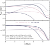 |
Fig. 1. Comparison of the evolution of the orbital parameters for the different scenarios explored by Rodríguez et al. (2021). Shown in dark blue are the results found with our modifications to the MESA source code, while in grey the results from Rodríguez et al. (2021). In the top (bottom) panel the evolution of Porb (e) is represented for different initial conditions (see legend). All three cases are described in more detail in Rodríguez et al. (2021). |
In contrast, for case II we obtain a faster declining Porb evolution. Compared to that work, this deviation starts at around 2 Myr and grows over time. Close to 2.5 Myr the binary achieves coplanarity, while synchronous orbit is reached at 3.8 Myr. Finally, at about 4 Myr the orbit becomes circular. However, our value of Porb is lower than that found by Rodríguez et al. (2021), likely due to differences in how AM is computed in our code with respect to theirs.
In addition, in the bottom panel of Fig. 1 we show that the evolution of e closely resembles the results of Rodríguez et al. (2021) in all the cases. Once again, in case II we find that our simulation evolves towards a circular orbit faster than theirs.
3. Results
In this section, we show the results on the evolution of different binary parameters subject to non-coplanar tides.
3.1. Mass transfer during core hydrogen burning
First, we model the evolution of a progenitor of a HMXB in which the MT between the star and the compact object occurs when the non-degenerate star is in the MS, called case A of MT (Kippenhahn & Weigert 1967). For this, we model a binary consisting of a 15 M⊙ BH in an eccentric orbit with e = 0.25 and Porb = 3 days, around a 20 M⊙ companion star. The star is assumed to be rotating at 0.9 of its critical rotation rate (Ω1/Ωcrit = 0.9). To understand the role of non-coplanarity, we explore several different inclinations between the spin of the star and the orbital AM, as well as the coplanar case of (i = 0).
The impact of different initial inclinations on Porb and e is shown in Fig. 2. It is clear that there is little change in Porb due to the inclination evolution. The most important changes occur at the beginning of the MS evolution of the star, where Porb increases faster for the smaller values of i. However, after half of the MS evolutionary timescale, the differences in Porb disappear. On the other hand, when studying the change in e, we see a clear difference before reaching a MT phase. In this case, inclinations higher than 90° are able to change the slope of the eccentricity derivative, leading to the different shapes shown in the bottom panel of Fig. 2. However, in all cases the binary tends to reach the equilibrium state characterized by a circular orbit in less than 70% of the MS evolutionary timescale.
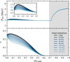 |
Fig. 2. Main sequence evolution of Porb (top panel) and e (bottom panel). Each shade of blue represents a detailed evolution assuming an initial inclination (see legend, bottom panel). The coplanar case (i = 0) is shown in black. The zoomed-in region in the top panel presents a clear picture of the different orbital periods around the first half of the MS evolution of the binaries. The grey region indicates the MT phase. |
We show the evolution of the inclination between the spin of the star and the orbital AM in Fig. 3, which reflects that the slope of i in function of time (t) varies according to its initial value. For all cases, we find that in less than 20% of the MS lifetime of the star the binary reaches coplanarity (i = 0), after which the equations derived by Hut (1981) are recovered. In addition, in Fig. 3 we present the evolution towards a synchronous orbit, by showing the ratio of the rotational period of the star, Prot, to Porb. Before reaching the equilibrium state, the rotational rate differs for different values of i, acquiring faster rotations for the smallest inclinations. Here it is clearly seen how this equilibrium condition is achieved at around half of the MS lifetime, thus safely allowing the use of the Roche formalism for the MT stage, which happens at around 70% of the MS lifetime.
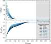 |
Fig. 3. Evolution during main sequence of i (top panel) and Prot/Porb (bottom panel). Each shade of blue represents a detailed evolution assuming an initial inclination (see legend, bottom panel). The coplanar case (i = 0) is shown in black. The case Prot/Porb = 1, which represents a synchronous orbit, is shown as a black dashed line. The grey region indicates the MT phase. |
From Figs. 2 and 3 we conclude that the non-coplanar tides acting on a tight binary in which its components interact during core-H burning push the binary to reach the equilibrium state before the start of the MT phase that characterizes an accreting HMXB.
3.2. Mass transfer after core hydrogen depletion
In order to study the impact of tides over a broad range of conditions, we also explore cases with a wider binary configuration. Here we present the results for the evolution of a binary with the same component masses, eccentricities, and rotational rates as in Sect. 3.1, but with a higher Porb of 50 days. For these cases the beginning of the MT phase occurs after the end of MS evolution, when the star crosses the Hertzsprung gap (HG), such that the MT is commonly referred to as case B of MT (Kippenhahn & Weigert 1967).
The evolution of Porb and e for different values of i are shown in Fig. 4. Similar to case A of MT, Porb behaves in an analogous manner for the different i values. There is, however, a small difference just before the start of the MT phase, as highlighted in the inset of the figure. For the evolution of e, shown in the bottom panel of Fig. 4, we see that its progress over time depends on the inclination, with smaller values of i favouring smaller changes towards a circular orbit. Hence, for this case of MT a circular orbit is reached a few hundred years after the start of the MT phase, around 9500 yr after the end of the MS evolution.
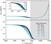 |
Fig. 4. Same parameter evolutions as in Fig. 2, but the time axis starts just after the end of the MS. The evolution of these parameters before ∼6000 yr after reaching the end of the MS is the same in all the different inclination cases. In the zoomed-in region the small differences present in Porb just before the beginning of the MT phase are shown. The grey region indicates the MT phase. |
Regarding the inclination evolution shown in Fig. 5, we see that it starts to change some thousands of years before the beginning of the MT phase, with the more abrupt changes related to the higher initial i values. This behaviour is a consequence of the increase in the radius of the star such that the ratio R1/a becomes more important in the equations presented in Sect. 2.1. All these cases tend to a coplanar state that is reached just after the start of the MT phase.
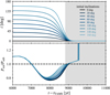 |
Fig. 5. Same parameter evolutions as in Fig. 3, but with a time axis as described in Fig. 4. The black dashed line represents the synchronous orbit. |
An important result found for this MT case is connected to the evolution of Prot/Porb (see bottom panel of Fig. 5). On the one hand, we find that ∼7000 yr after the end of the MS the star begins to rotate at a faster rate than Porb, but this tendency is reverted during the last thousand years before the start of the MT phase. On the other hand, during the first hundred years of the MT phase, the star does not have a totally synchronous orbit. This equilibrium state is briefly achieved until the clear slow down of the spin of the star occurring around ∼9500 yr after the MS.
Thus, we can conclude that the different initial values of i reach equilibrium conditions on a similar timescale, but the evolution towards those conditions can be very different, as in the cases of e and Prot/Porb.
3.3. Different physical assumptions
To explore a wider range of conditions that could modify the evolution of the binaries, we computed a set of models in which the initial binary conditions are fixed, with masses MBH = 15 M⊙ and M1 = 20 M⊙, in an eccentric orbit of e = 0.25 and Porb = 3 days and an inclination of i = 80 deg. We explore two different initial rotation velocities Ω1/Ωcrit = 0.1, 0.9, and for each of these cases we turn on and off the contribution of the ST dynamo to the AM transport (respectively labelled in Fig. 6 as ‘with ST’ and ‘without ST’).
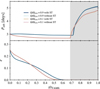 |
Fig. 6. Same evolution as in Fig. 2, but for different conditions in the spin of the star and the AM transport (see legend, top panel). |
The different results for the evolution of Porb and e are presented in Fig. 6. We see that the main difference arises when the initial spins are changed. This behaviour is maintained even after the MT starts as Porb is shorter for the initially less rapidly rotating star. The impact of using the ST dynamo seems to be negligible for these two orbital parameters. In the bottom panel of Fig. 6 we show that the condition of circularity is reached first for the slowly rotating case.
However, whether the ST dynamo is considered or not can be seen when studying the evolution of the spin of the star. In Fig. 7 we can see this difference in the AM transport becoming important during the MT phase, as the ratio Prot/Porb shows a clear change in its value when this contribution is turned on and off.
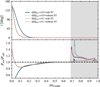 |
Fig. 7. Same evolution as in Fig. 3, but for different conditions in the spin of the star and the AM transport (see legend, top panel). The black dashed line represents a synchronous orbit. |
Overall, the impact of the spin of the star is much more important during the evolution prior to the start of the MT phase, as is expected, due to the explicit dependence in the tidal equations (Sect. 2.1). Instead, the AM transport becomes relevant once the MT has started, and the binary has reached the equilibrium state.
4. Summary and conclusions
At the end of their evolution, most massive stars go through a core collapse to form a compact object, which could be a NS or a BH. This formation is often associated with very powerful astrophysical transients such as supernovae and gamma-ray bursts. Many physical processes operating during this short-lived stage still remain unknown, one important process being whether this core collapse is symmetric or not. This dichotomy can be seen in the momentum kick imparted to the newly born object, although the presence of this kick may depend on the nature of the compact object, with NSs having well-constrained kick magnitudes (Hobbs et al. 2005), while kicks in BHs are more uncertain (Brandt et al. 1995; Willems et al. 2005; Wong et al. 2012, 2014; Vanbeveren et al. 2020; Callister et al. 2021; Stevenson 2022). In addition, if these stars are members of binary systems, the momentum kick imparted to the remnant will, through linear momentum conservation, modify the orbital parameters of the binary: Porb, e, and i. After that, the orbital and internal AM evolution will be dominated by the effect of tides operating on the binary system.
In this work we address the topic of how these tides operate on the progenitors of HMXBs in which, after such an asymmetric kick is imparted, the spin of the star is not aligned with the orbital AM. For this purpose, we include the formulation of Repetto & Nelemans (2014) for arbitrary inclinations in the stellar evolution code MESA. With this tool, we study the evolution of the binary parameters considering different initial values of the inclination between the AM of the star and the orbital plane i for cases A and B of MT (Kippenhahn & Weigert 1967).
For the evolution through both cases of MT, we note that the most noticeable differences arise in the evolution of e, i, and Prot. The changes in these parameters are driven by tidal coupling, which forces the system to evolve towards an equilibrium state characterized by circularization, coplanarity, and synchronous orbit. This state is achieved faster for the more compact binary (i.e. the conditions of case A of MT) as a consequence of the strong dependence of tides with the separation between the binary members (see Sect. 2.1).
Furthermore, in this work we explored the role of the initial spin on the subsequent binary evolution. We find the spin to be an important variable that regulates the timescale for each of the different conditions of the equilibrium state. We also study an important yet debated mechanism of AM transport: the ST dynamo. As already shown by other authors (Qin et al. 2019) its absence could help to explain the high spin measured in the BHs of HMXBs, although this might not be consistent with the population of BHs detected by the LIGO and Virgo collaboration (Abbott et al. 2021). In this work we find that the role of this mechanism is secondary when analysing the change on the binary parameters due to tidal evolution, although it becomes important once a binary reaches the onset of a MT phase. However, the ST dynamo might play an important role in scenarios where a rapidly rotating core of a star is needed at the end of the evolution to reproduce energetic transient events (Fuller & Lu 2022).
Many physical uncertainties could affect our results across this modelling. Understanding the impact of such limitations is a key factor. On the one hand, the set of non-linear differential equations that describe the evolution of the semi-major axis, eccentricity, rotation rate, and inclination of the rotation axis with respect to the orbital plane, as presented by Repetto & Nelemans (2014), is considered until the onset of a MT phase. Once a star is near to filling its Roche lobe, the quadrupolar terms in the perturbation theory of tides of Hut (1981) might stop being a good approximation, with tides becoming stronger than predicted. Moreover, the Roche formalism requires synchronous orbit between the components of the binary and Porb; in our case B of MT, we find small deviations of the synchronous orbit state at the beginning of the MT phase which is rapidly achieved during the first years of MT. Lastly, the transport of AM is also uncertain and will certainly have an impact on the results during the MT phase. There is observational evidence that this transport is highly efficient such that most stars end their evolution with a smaller content of AM than predicted (Cantiello et al. 2014; Fuller et al. 2014, 2019; Spada et al. 2016; Aerts et al. 2019; Eggenberger et al. 2019; den Hartogh et al. 2019). Although this is particularly true for measurements of BHs with low spin values (Abbott et al. 2021), there seem to be HMXBs containing BHs with high spin values (Miller & Miller 2015). This issue is currently under debate (Qin et al. 2019; Bavera et al. 2020; Fishbach & Kalogera 2022; Belczynski et al. 2021).
The results of this study show that prior to the X-ray binary phase, the evolution of the orbital parameters differ according to the value of the inclination of the rotational axis with respect to the orbital plane. Thus, for some binaries, matching observed quantities with those coming from stellar evolution simulations might help constrain the conditions at core collapse, as well as the momentum kick imparted to the newly born compact object.
The modified version of the code can be found in the following GitHub repository: https://github.com/asimazbunzel/non-coplanar-tides
Acknowledgments
A.S.B. is a fellow of CONICET. F.G. and J.A.C. are CONICET researchers. F.G. and J.A.C. acknowledge support by PIP 0113 (CONICET). J.A.C. is a María Zambrano researcher fellow funded by the European Union -NextGenerationEU- (UJAR02MZ). This work received financial support from PICT-2017-2865 (ANPCyT). J.A.C. was also supported by grant PID2019-105510GB-C32/AEI/10.13039/501100011033 from the Agencia Estatal de Investigación of the Spanish Ministerio de Ciencia, Innovación y Universidades, and by Consejería de Economía, Innovación, Ciencia y Empleo of Junta de Andalucía as research group FQM- 322, as well as FEDER funds. S.C. acknowledges the CNES (Centre National d’Etudes Spatiales) for the funding of MINE (Multi-wavelength INTEGRAL Network). A.S.B., F.G., F.F. and S.C. are grateful to the LabEx UnivEarthS for the funding of Interface project I10 “From binary evolution towards merging of compact objects”. Software: MESA (http://mesa.sourceforge.net/) (Paxton et al. 2011, 2013, 2015; Paxton et al. 2018, 2019), ipython/jupyter (Kluyver et al. 2016), matplotlib (Hunter 2007), numpy (Harris et al. 2020).
References
- Abbott, R., Abbott, T. D., Abraham, S., et al. 2021, Phys. Rev. X, 11, 021053 [Google Scholar]
- Aerts, C., Mathis, S., & Rogers, T. M. 2019, ARA&A, 57, 35 [Google Scholar]
- Alexander, M. E. 1973, Ap&SS, 23, 459 [NASA ADS] [CrossRef] [Google Scholar]
- Bavera, S. S., Fragos, T., Qin, Y., et al. 2020, A&A, 635, A97 [NASA ADS] [CrossRef] [EDP Sciences] [Google Scholar]
- Belczynski, K., Kalogera, V., Rasio, F. A., et al. 2008, ApJS, 174, 223 [Google Scholar]
- Belczynski, K., Klencki, J., Fields, C. E., et al. 2020, A&A, 636, A104 [NASA ADS] [CrossRef] [EDP Sciences] [Google Scholar]
- Belczynski, K., Done, C., & Lasota, J. P. 2021, ArXiv e-prints [arXiv:2111.09401] [Google Scholar]
- Blaauw, A. 1961, Bull. Astron. Inst. Neth., 15, 265 [NASA ADS] [Google Scholar]
- Böhm-Vitense, E. 1958, ZAp, 46, 108 [NASA ADS] [Google Scholar]
- Brandt, W. N., Podsiadlowski, P., & Sigurdsson, S. 1995, MNRAS, 277, L35 [NASA ADS] [Google Scholar]
- Brott, I., de Mink, S. E., Cantiello, M., et al. 2011, A&A, 530, A115 [NASA ADS] [CrossRef] [EDP Sciences] [Google Scholar]
- Burrows, A., Hayes, J., & Fryxell, B. A. 1995, ApJ, 450, 830 [NASA ADS] [CrossRef] [Google Scholar]
- Callister, T. A., Farr, W. M., & Renzo, M. 2021, ApJ, 920, 157 [NASA ADS] [CrossRef] [Google Scholar]
- Cantiello, M., Mankovich, C., Bildsten, L., Christensen-Dalsgaard, J., & Paxton, B. 2014, ApJ, 788, 93 [Google Scholar]
- Darwin, G. H. 1879, Philos. Trans. R. Soc. London Ser. I, 170, 1 [NASA ADS] [Google Scholar]
- den Hartogh, J. W., Eggenberger, P., & Hirschi, R. 2019, A&A, 622, A187 [NASA ADS] [CrossRef] [EDP Sciences] [Google Scholar]
- Eggenberger, P., Deheuvels, S., Miglio, A., et al. 2019, A&A, 621, A66 [NASA ADS] [CrossRef] [EDP Sciences] [Google Scholar]
- Fishbach, M., & Kalogera, V. 2022, ApJ, 929, L26 [NASA ADS] [CrossRef] [Google Scholar]
- Fuller, J., & Lu, W. 2022, MNRAS, 511, 3951 [NASA ADS] [CrossRef] [Google Scholar]
- Fuller, J., Lecoanet, D., Cantiello, M., & Brown, B. 2014, ApJ, 796, 17 [Google Scholar]
- Fuller, J., Piro, A. L., & Jermyn, A. S. 2019, MNRAS, 485, 3661 [NASA ADS] [Google Scholar]
- Goldreich, P., & Nicholson, P. D. 1977, Icarus, 30, 301 [NASA ADS] [CrossRef] [Google Scholar]
- Grevesse, N., & Sauval, A. J. 1998, Space Sci. Rev., 85, 161 [Google Scholar]
- Harris, C. R., Millman, K. J., van der Walt, S. J., et al. 2020, Nature, 585, 357 [NASA ADS] [CrossRef] [Google Scholar]
- Heger, A., Langer, N., & Woosley, S. E. 2000, ApJ, 528, 368 [NASA ADS] [CrossRef] [Google Scholar]
- Herant, M., Benz, W., Hix, W. R., Fryer, C. L., & Colgate, S. A. 1994, ApJ, 435, 339 [NASA ADS] [CrossRef] [Google Scholar]
- Hobbs, G., Lorimer, D. R., Lyne, A. G., & Kramer, M. 2005, MNRAS, 360, 974 [Google Scholar]
- Hoyle, F., & Fowler, W. A. 1960, ApJ, 132, 565 [NASA ADS] [CrossRef] [Google Scholar]
- Hunter, J. D. 2007, Comput. Sci. Eng., 9, 90 [NASA ADS] [CrossRef] [Google Scholar]
- Hurley, J. R., Tout, C. A., & Pols, O. R. 2002, MNRAS, 329, 897 [Google Scholar]
- Hut, P. 1981, A&A, 99, 126 [NASA ADS] [Google Scholar]
- Janka, H.-T. 2012, Annu. Rev. Nucl. Part. Sci., 62, 407 [NASA ADS] [CrossRef] [Google Scholar]
- Janka, H. T., & Mueller, E. 1996, A&A, 306, 167 [NASA ADS] [Google Scholar]
- Kalogera, V. 1996, ApJ, 471, 352 [Google Scholar]
- Keil, W., Janka, H. T., & Mueller, E. 1996, ApJ, 473, L111 [NASA ADS] [CrossRef] [Google Scholar]
- Kippenhahn, R., & Weigert, A. 1967, ZAp, 65, 251 [Google Scholar]
- Kippenhahn, R., Ruschenplatt, G., & Thomas, H. C. 1980, A&A, 91, 175 [Google Scholar]
- Kluyver, T., Ragan-Kelley, B., Pérez, F., et al. 2016, in Positioning and Power in Academic Publishing: Players, Agents and Agendas, eds. F. Loizides, & B. Schmidt (IOS Press), 87 [Google Scholar]
- Kolb, U., & Ritter, H. 1990, A&A, 236, 385 [NASA ADS] [Google Scholar]
- Kotake, K., Yamada, S., & Sato, K. 2003, ApJ, 595, 304 [NASA ADS] [CrossRef] [Google Scholar]
- Landau, L. D., & Lifshitz, E. M. 1975, The Classical Theory of Fields (Oxford: Pergamon Press) [Google Scholar]
- Langer, N., Fricke, K. J., & Sugimoto, D. 1983, A&A, 126, 207 [NASA ADS] [Google Scholar]
- Ledoux, P. 1947, ApJ, 105, 305 [NASA ADS] [CrossRef] [Google Scholar]
- Marchant, P., Langer, N., Podsiadlowski, P., et al. 2017, A&A, 604, A55 [NASA ADS] [CrossRef] [EDP Sciences] [Google Scholar]
- Miller, M. C., & Miller, J. M. 2015, Phys. Rep., 548, 1 [NASA ADS] [CrossRef] [Google Scholar]
- Olejak, A., & Belczynski, K. 2021, ApJ, 921, L2 [NASA ADS] [CrossRef] [Google Scholar]
- Paczyński, B. 1998, ApJ, 494, L45 [Google Scholar]
- Paxton, B., Bildsten, L., Dotter, A., et al. 2011, ApJS, 192, 3 [Google Scholar]
- Paxton, B., Cantiello, M., Arras, P., et al. 2013, ApJS, 208, 4 [Google Scholar]
- Paxton, B., Marchant, P., Schwab, J., et al. 2015, ApJS, 220, 15 [Google Scholar]
- Paxton, B., Schwab, J., Bauer, E. B., et al. 2018, ApJS, 234, 34 [NASA ADS] [CrossRef] [Google Scholar]
- Paxton, B., Smolec, R., Schwab, J., et al. 2019, ApJS, 243, 10 [Google Scholar]
- Petrovic, J., Langer, N., Yoon, S. C., & Heger, A. 2005, A&A, 435, 247 [NASA ADS] [CrossRef] [EDP Sciences] [Google Scholar]
- Qin, Y., Fragos, T., Meynet, G., et al. 2018, A&A, 616, A28 [NASA ADS] [CrossRef] [EDP Sciences] [Google Scholar]
- Qin, Y., Marchant, P., Fragos, T., Meynet, G., & Kalogera, V. 2019, ApJ, 870, L18 [Google Scholar]
- Qin, Y., Shu, X., Yi, S., & Wang, Y. Z. 2022a, RAA, 22, 3 [Google Scholar]
- Qin, Y., Wang, Y.-Z., Wu, D.-H., Meynet, G., & Song, H. 2022b, ApJ, 924, 129 [NASA ADS] [CrossRef] [Google Scholar]
- Repetto, S., & Nelemans, G. 2014, MNRAS, 444, 542 [NASA ADS] [CrossRef] [Google Scholar]
- Rodríguez, C. N., Ferrero, G. A., Benvenuto, O. G., et al. 2021, MNRAS, 508, 2179 [CrossRef] [Google Scholar]
- Scheck, L., Kifonidis, K., Janka, H. T., & Müller, E. 2006, A&A, 457, 963 [NASA ADS] [CrossRef] [EDP Sciences] [Google Scholar]
- Soberman, G. E., Phinney, E. S., & van den Heuvel, E. P. J. 1997, A&A, 327, 620 [NASA ADS] [Google Scholar]
- Spada, F., Gellert, M., Arlt, R., & Deheuvels, S. 2016, A&A, 589, A23 [NASA ADS] [CrossRef] [EDP Sciences] [Google Scholar]
- Spruit, H. C. 2002, A&A, 381, 923 [CrossRef] [EDP Sciences] [Google Scholar]
- Stevenson, S. 2022, ApJ, 926, L32 [NASA ADS] [CrossRef] [Google Scholar]
- Vanbeveren, D., Mennekens, N., van den Heuvel, E. P. J., & Van Bever, J. 2020, A&A, 636, A99 [NASA ADS] [CrossRef] [EDP Sciences] [Google Scholar]
- Willems, B., Henninger, M., Levin, T., et al. 2005, ApJ, 625, 324 [NASA ADS] [CrossRef] [Google Scholar]
- Wong, T.-W., Valsecchi, F., Fragos, T., & Kalogera, V. 2012, ApJ, 747, 111 [NASA ADS] [CrossRef] [Google Scholar]
- Wong, T.-W., Valsecchi, F., Ansari, A., et al. 2014, ApJ, 790, 119 [NASA ADS] [CrossRef] [Google Scholar]
- Woosley, S. E. 1993, ApJ, 405, 273 [Google Scholar]
- Zahn, J. P. 1975, A&A, 41, 329 [NASA ADS] [Google Scholar]
- Zahn, J. P. 1977, A&A, 57, 383 [Google Scholar]
- Zahn, J. P. 2008, in EAS Publications Series, eds. M. J. Goupil, & J. P. Zahn, 29, 67 [NASA ADS] [CrossRef] [EDP Sciences] [Google Scholar]
All Figures
|
Fig. 1. Comparison of the evolution of the orbital parameters for the different scenarios explored by Rodríguez et al. (2021). Shown in dark blue are the results found with our modifications to the MESA source code, while in grey the results from Rodríguez et al. (2021). In the top (bottom) panel the evolution of Porb (e) is represented for different initial conditions (see legend). All three cases are described in more detail in Rodríguez et al. (2021). |
| In the text | |
|
Fig. 2. Main sequence evolution of Porb (top panel) and e (bottom panel). Each shade of blue represents a detailed evolution assuming an initial inclination (see legend, bottom panel). The coplanar case (i = 0) is shown in black. The zoomed-in region in the top panel presents a clear picture of the different orbital periods around the first half of the MS evolution of the binaries. The grey region indicates the MT phase. |
| In the text | |
|
Fig. 3. Evolution during main sequence of i (top panel) and Prot/Porb (bottom panel). Each shade of blue represents a detailed evolution assuming an initial inclination (see legend, bottom panel). The coplanar case (i = 0) is shown in black. The case Prot/Porb = 1, which represents a synchronous orbit, is shown as a black dashed line. The grey region indicates the MT phase. |
| In the text | |
|
Fig. 4. Same parameter evolutions as in Fig. 2, but the time axis starts just after the end of the MS. The evolution of these parameters before ∼6000 yr after reaching the end of the MS is the same in all the different inclination cases. In the zoomed-in region the small differences present in Porb just before the beginning of the MT phase are shown. The grey region indicates the MT phase. |
| In the text | |
|
Fig. 5. Same parameter evolutions as in Fig. 3, but with a time axis as described in Fig. 4. The black dashed line represents the synchronous orbit. |
| In the text | |
|
Fig. 6. Same evolution as in Fig. 2, but for different conditions in the spin of the star and the AM transport (see legend, top panel). |
| In the text | |
|
Fig. 7. Same evolution as in Fig. 3, but for different conditions in the spin of the star and the AM transport (see legend, top panel). The black dashed line represents a synchronous orbit. |
| In the text | |
Current usage metrics show cumulative count of Article Views (full-text article views including HTML views, PDF and ePub downloads, according to the available data) and Abstracts Views on Vision4Press platform.
Data correspond to usage on the plateform after 2015. The current usage metrics is available 48-96 hours after online publication and is updated daily on week days.
Initial download of the metrics may take a while.