| Issue |
A&A
Volume 669, January 2023
|
|
|---|---|---|
| Article Number | A157 | |
| Number of page(s) | 13 | |
| Section | Stellar atmospheres | |
| DOI | https://doi.org/10.1051/0004-6361/202244771 | |
| Published online | 27 January 2023 | |
Small-scale dynamo in cool stars
II. The effect of metallicity
Max Planck Institute for Solar System Research,
Justus-von-Liebig-Weg 3,
37077
Göttingen, Germany
e-mail: This email address is being protected from spambots. You need JavaScript enabled to view it.
Received:
18
August
2022
Accepted:
17
November
2022
Abstract
Context. All cool main sequence stars including our Sun are thought to have magnetic fields. Observations of the Sun revealed that small-scale turbulent magnetic fields are present even in quiet regions. Simulations further showed that such magnetic fields affect the subsurface and photospheric structure, and thus the radiative transfer and emergent flux. Since small-scale turbulent magnetic fields on other stars cannot be directly observed, it is imperative to numerically study their effects on the near surface layers.
Aims. Until recently comprehensive three-dimensional simulations capturing the effect of small-scale turbulent magnetic fields only exist for the solar case. A series of investigations extending small-scale dynamo simulations for other stars has been started. Here we aim to examine small-scale turbulent magnetic fields in stars of solar effective temperature but different metallicity.
Methods. We investigate the properties of three-dimensional simulations of the magneto-convection in boxes covering the upper convection zone and photosphere carried out with the MURaM code for metallicity values of M/H = {–1.0,0.0,0.5} with and without a small-scale dynamo.
Results. We find that small-scale turbulent magnetic fields enhanced by a small-scale turbulent dynamo noticeably affect the subsurface dynamics and significantly change the flow velocities in the photosphere. Moreover, significantly stronger magnetic field strengths are present in the convection zone for low metallicity. Instead, at the optical surface the averaged vertical magnetic field ranges from 64G for M/H = 0.5 to 85G for M/H = –1.0.
Key words: methods: numerical / magnetohydrodynamics (MHD) / convection / stars: magnetic field / stars: atmospheres / stars: interiors
© The Authors 2023
 Open Access article, published by EDP Sciences, under the terms of the Creative Commons Attribution License (https://creativecommons.org/licenses/by/4.0), which permits unrestricted use, distribution, and reproduction in any medium, provided the original work is properly cited.
This article is published in open access under the Subscribe-to-Open model.
Open access funding provided by Max Planck Society.
1 Introduction
Atmospheres of cool stars, which are stars with convective envelopes like the Sun, are filled with magnetic fields. Some of these fields emerge from below the stellar surface and affect the structure of the stellar atmosphere, changing the radiative emission from the star. The various manifestations of such atmospheric changes, for example spectroscopic and brightness variations and Ca II and X-ray emission and their variations (see e.g. Schrijver & Zwaan 2000, and references therein), are usually referred to as stellar magnetic activity.
The interest in stellar activity is not at all limited to solar and stellar physics. Stellar brightness variability is also a limiting factor in the detection and characterisation of exoplanets by transit-photometry missions (Aigrain et al. 2004; Johnson et al. 2021). The magnetic jitter in radial velocity affects the spectroscopic detection of planets (Fischer et al. 2016; Meunier & Lagrange 2019), while the magnetic jitter in position of the stellar brightness centre impedes the astrometric detection of planets (Meunier et al. 2020; Sowmya et al. 2021; Kaplan-Lipkin et al. 2021). Recent studies have also shown that magnetic features on stellar surfaces can substantially interfere with identifying the chemical composition of exoplanetary atmospheres by transmission spectroscopy (Rackham et al. 2018, 2019).
The star whose surface magnetic field has been most extensively studied is the Sun (see e.g. the review by Solanki et al. 2006, and references therein). Observations show that the most salient manifestations of solar surface magnetism, such as spots, faculae, and magnetic networks, are modulated by the activity cycle produced by the action of the global dynamo in the interior of the Sun (Charbonneau 2020). Surprisingly, it was also revealed that even the solar regions free from any apparent manifestation of magnetic activity (i.e. the quiet Sun) are interspersed with small-scale magnetic fields of mixed polarity (often also referred as ‘internetwork’ magnetic fields; see Livingston & Harvey 1975), which appear to be largely uncorrelated with the solar cycle (see reviews by Buehler et al. 2013; Lites et al. 2014; Borrero et al. 2017; Bellot Rubio & Orozco Suárez 2019).
These fields lead to considerable small-scale turbulent magnetic flux that is always present at the solar surface (Trujillo Bueno et al. 2004). Simulations can successfully explain their existence by the action of a small-scale dynamo (SSD), which describes the amplification of the magnetic flux by the near-surface turbulent convection (see Rempel 2018, and references therein). Interestingly, it was recently shown that small-scale internetwork magnetic fields amplified by a turbulent dynamo have a significant effect on the radiation emanating from the Sun (Rempel 2020; Yeo et al. 2020). This raises a compelling question of whether small-scale fields can also affect photometric and spectral stellar data. There is presently no answer to this question since nothing is currently known about the properties of the small-scale turbulent magnetic fields on stars others than the Sun. In particular, their effect on stellar atmospheres was not considered in the widely used 1D (e.g. Castelli & Kurucz 2003; Gustafsson et al. 2008; Husser et al. 2013) and 3D (e.g. Ludwig et al. 2009; Beeck et al. 2013; Magic et al. 2013) grids of stellar atmospheric models.
This is the second study in a series of papers where we correct this omission and investigate the properties and effects of magnetic fields generated by small-scale turbulent dynamos in stars with outer convection zones. In a parallel study we investigate the SSD as a function of the stellar effective temperature (Bhatia et al. 2022), where we focused on stars of spectral types F3V, G2V, K0V, and M0V with solar metallicity. In this paper we utilised the MURaM code (Vögler et al. 2005) to simulate the action of SSD and small-scale fields in metal-rich (M/H = 0.5) and metal-poor (M/H = –1.0) stars with solar temperature and surface gravity. We further investigated the backreaction of the SSD on the near-surface convection and structure of stellar atmosphere. For comparison we also perform simulations for the Sun (M/H = 0.0). In the forthcoming papers we will consider the effects of SSD on stellar measurements.
The paper is structured as follows. The numerical model is described in Sect. 2, where we give the governing equations and the simulation set-up. Subsequently, we present our results in Sect. 3 and discuss their implications in Sect. 4.
2 Model
In this study we follow the ‘box-in-a-star’ approach. We consider a Cartesian box filled with plasma that represents a small part of a star around the optical surface, such that the upper convection zone and the photosphere are included.
2.1 Governing equations and implementation
To solve for the dynamics and energy transport in such a region we employ the radiative 3D magnetohydrodynamic (MHD) code MURaM (Vögler et al. 2005; Rempel 2014, 2016), which uses a fourth-order accurate conservative, centred finite scheme for the discretisation. For the radiative transfer a multi-group scheme with short characteristics is implemented (Nordlund 1982). A pre-tabulated equation of state is used, which we generated with the FreeEOS code (Irwin 2012).
MURaM solves the conservative MHD equations for a compressible partially ionised plasma in the following form:
 (1)
(1)
 (2)
(2)
 (3)
(3)
 (4)
(4)
 (5)
(5)
Here, ρ is the density, p the pressure, u the velocity, B the magnetic field, Qrad and Qres the radiative heating term and the resistive heating term, and g the gravitational acceleration, which in this study is set to log ɡ = 4.4378. The force term FL is the Lorentz force and FSR denotes the semi-relativistic (Boris) correction (Boris 1970; Gombosi et al. 2002), which is negligible for our set-up. The hydrodynamic energy, EHD, is the sum of the internal energy (Eint) and the kinetic energy (EHD) = Eint + 1/2ρu2). In order to achieve numerical stability it is necessary to implement an additional diffusion scheme. The implementation in MURaM is based on a slope-limited diffusion scheme, where the diffusive terms are implemented in terms of fluxes of the conserved quantities across the grid-cell boundaries (for a detailed description, see Rempel 2014, 2016).
2.2 Boundary conditions
The simulation domain is periodic in both the horizontal (x and y) directions and has boundaries at the top and bottom (ztop, zbottom). In addition to the cells within the domain, two ghost cells at the top and bottom boundaries are introduced. These are needed for the implementation of the vertical derivatives and the boundary conditions. For most variables a closed or open boundary is achieved using symmetric and antisymmetric neighbouring ghost cells at the boundary. For any variable υ in a symmetric implementation, the two ghost cells  (the tilde denotes the ghost cells), where
  is the one next to the boundary, are set to corresponding values in the domain
  . Instead, for an anti-symmetric case the condition reads
  .
.
The top boundary permits outflows (symmetric), but inflows (anti-symmetric) are not allowed. In addition, ztop is open to vertical magnetic fields. The formulation of the bottom boundary condition affects the magnetic field generation. In the past, different conditions were tested, ranging from boundary conditions that ensure a self-contained dynamo problem to various settings to mimic the deep convection zone (Rempel 2014). Based on equipartition arguments it was shown that some boundary conditions mimic the structure of magnetic field deeper in the convection zone more consistently (Rempel 2014; Hotta et al. 2015). Consequently, we consider boundary conditions similar to those in Rempel (2014), where zbottom is open to mass flux (ρuz) and magnetic fields. We note that an open boundary condition for magnetic fields might lead to violation of the divergence-free constraint. To generally counter the build up of deviations from ∇ B = 0, MURaM uses a hyperbolic divergence cleaning approach (Dedner et al. 2002).
To maintain an average constant effective temperature of the simulation, the entropy inflow is specified at the bottom boundary, sbc, while the entropy down-flows are symmetric. The pressure at the boundary and at the ghost cells is treated as described for the HD2 condition in Rempel (2016), where the gas pressure is split into a mean pressure plus fluctuations,  . However, we use a slightly different damping factor Cdmp = 0.8 and add additional damping proportional to magnetic pressure. Then, our extrapolation to ghost cells reads
 (6)
(6)
 (7)
(7)
where pbc is the fixed pressure value that we aim to maintain at the bottom and  is the vertical magnetic field at the first ghost cell (i.e. due to the symmetric condition
  ). A list of the boundary conditions is given in Table 1.
2.3 Simulation set-up
The horizontal extent of our simulation box is 9 Mm × 9 Mm and it is chosen to contain at least a dozen granulation cells. The vertical extent is 5 Mm so that the box covers the photosphere (roughly up to the temperature minimum) and reaches down to the upper convection zone (~4 Mm below the optical surface, τ500 = 1 ). While the box has an extent of 1 Mm above the surface the top layers are affected by the top boundary condition, which is open to vertical magnetic fields. We estimate that the dynamics in roughly 0.5 Mm from the top might be influenced by this choice of boundary condition, and we indicate this by a grey shaded area in all plots. The numerical grid has 500 points in the vertical and 512 × 512 points in the horizontal direction. The element composition of the plasma is taken from Asplund et al. (2009). In this study we restrict the analysis to three different metallicity values (M/H = –1.0, 0.0, and 0.5), where compared to the Sun M/H = –1.0 corresponds to ten times lower metallicity and M/H = 0.5 to approximately three times higher.
We used a 1D mean atmospheric structures generated by the Modules for Experiments in Stellar Astrophysics (MESA) code (Paxton et al. 2011) to initialise all three metallicity runs. After a simulation is initialised, it is run until it reaches a saturated state. For the SSD run, we inserted a small, random, and flux free magnetic field. Subsequently, the calculation was run until the root mean square (rms) magnetic field strength of the entire cube saturated. At the early stage, during the relaxation of the simulation, we used grey radiative transfer. Finally, we switched to a four-bin non-grey opacity table (for a more detailed discussion, see Vögler et al. 2004), where we updated the pre-tabulated opacity table according to the mean time averaged atmospheric structure several times.
Subsequently, the entropy and pressure values at the bottom boundary were adjusted iteratively. The pressure at the bottom was chosen such that the mean optical surface was roughly four Mm above the bottom of the box. Furthermore, the entropy inflow at the bottom was adjusted such that a time averaged mean effective temperature in the non-grey SSD run was maintained around 5777 K ± 15 K. The pressure and entropy conditions at the bottom, found to satisfy the above condition in the SSD run, were kept for the pure hydrodynamic run of the same metallicity value. Finally, we let the simulation evolve for ten hours of solar time.
Top and bottom boundary conditions.
3 Results
The 1D structures we show in this section were obtained by first averaging the 3D cubes in both horizontal directions. Subsequently, we took a time average over a series of snapshots over an interval of ten hours of solar simulation time (the typical number of snapshots is of order 103).
3.1 Effect of metallicity on stratification of SSD and hydro runs
In the following we consider the effect of metallicity on the stratification in the SSD simulations as well as the differences between SSD and pure hydrodynamic simulations. Overall, higher metallicity corresponds to greater opacity and leads to less efficient radiative transport of energy.
We now focus on changes in temperature and density stratification. Figure 1 shows the averaged 1D temperature with height, where we shifted the mean optical surface (τ500 = 1) to z = 0 for each of the metallicity runs. In addition, one standard deviation, σ, over the temporal variation is plotted as a shaded area. If not otherwise stated, shifts of the mean optical surface and the one standard deviation are present in all figures of 1D structures. Since the mean effective temperature for the three metallicity runs is almost the same (see Table 2), the temperature values in the vicinity of τ500 = 1 are similar. The low metallicity run (M/H = −1.0) shows a flatter temperature gradient just below the surface compared to the solar and the M/H = 0.5 run, but towards the deep layers in the convection zone the temperature shows a steeper increase compared to other metallicities. This can be explained by a somewhat lower pressure scale height for the M/H = −1.0 run (see Appendix A).
For the low metallicity run the photospheric temperature averaged over the horizontal extent of the box and time decreases more strongly just above the surface, but then it flattens out while higher metallicity runs produce a slightly steeper temperature gradient. For a more detailed illustration of the changes in the temperature gradient see Fig. A.1. The differences in the temperature gradients around the optical surface and the significantly different temperature profiles in the photosphere with different metallicity are expected to noticeably change the emerging spectra. In particular, H− is sensitive to small temperature changes, and thus is expected to result in differences in the continuum opacities. These differences will affect the energy distribution in the emergent intensities. In addition, temperature changes in the higher layers of the photosphere are expected to affect centre-to-limb variations.
We note that while the dependencies of the atmospheric structures on M/H discussed above have already been investigated in pure hydrodynamic simulations (see e.g. Ludwig et al. 2009; Magic et al. 2013) our calculations are the first to include SSD for stars with non-solar M/H. Along the same lines, previous studies (see e.g. Magic et al. 2013, 2015) of spectra and limb darkening dependencies on metallicity were performed without accounting for the effects of small-scale turbulent magnetic fields. We will perform a detailed analysis of these effects on emergent radiation for different metallicity values in a separate paper; here we focus on changes in the atmospheric structure and dynamics introduced by the action of SSD and the resulting small-scale turbulent magnetic field.
To pinpoint the effects of SSD, we calculated the temperature deviations in the averaged structures obtained from the SSD run to the hydro run. Figure 2 shows that SSD heats the gas both below and above the optical surface. Keeping in mind that the bottom boundary conditions are the same for the HD and the SSD runs for each metallicity, this implies a greater energy flux in the SSD calculations that leads to a slight increase in the effective temperature, but mainly to excess heating in the upper photosphere, typical of magnetic flux concentrations. This can be seen in Table 2 from the effective temperature averaged over time together with one standard deviation. We note that while the difference between the effective temperatures for the HD and the SSD runs are within a standard deviation (i.e. fluctuations in effective temperature from one time step to another due to convection are stronger than the permanent changes in Teff due to a SSD), the values are significantly different: the error of the mean is much smaller than the standard deviation. At the surface, the increased heat flux in the SSD simulations can be explained by the magnetic regions being evacuated, which results in a density drop. The lower density in such magnetic regions allows for a more efficient radiative transport because the opacity decreases. This in turn results in extra heating from hotter non-magnetic surroundings (see Solanki et al. 2013, and references therein). Basically, the solar surface area is increased, and so more radiation can escape.
Below the optical surface, changes in pressure and density in the SSD run (Fig. 2) compared to the pure hydrodynamic simulation are rather insensitive to the metallicity and can be explained by the magnetic pressure and change in the turbulent pressure (see Bhatia et al. 2022, for a more detailed discussion). Higher up in the photosphere the changes in density and pressure depend significantly on the metallicity of the star.
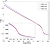 |
Fig. 1 Horizontally and time averaged temperature structure of the SSD runs with height for different metallicity values. The grey shaded area shows the region that might be affected by the top boundary conditions (see detailed discussion in Sect. 2.3). |
Mean effective temperature and analysis of the entropy profiles.
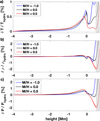 |
Fig. 2 Deviations in stratification from a pure hydro run to a SSD run: (a) temperature deviations; (b) density deviations; (c) pressure deviations. The grey shaded area is as defined in Fig. 1. |
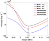 |
Fig. 3 Horizontally and time averaged entropy with height for the SSD simulations. The mean optical surface for all three runs is at z = 0. The vertical dash-dotted lines indicate the position of the local entropy minima. |
3.2 Entropy and convection efficiency
To quantify the effect of metallicity on convection we first calculated the entropy profiles with height using the averaged density and internal energy profiles. Figure 3 shows the entropy minima and their positions for different metallicity values. The entropy minima are associated with the height at which the convection zone ends. It becomes evident that with decreasing metallicity the convective region extends further above the mean optical surface.
The entropy change, ΔS, also called entropy jump, between the lower boundary (which corresponds to the constant entropy value present in the adiabatic convection zone) and the entropy minima can be used as an indicator of the convection efficiency (Magic et al. 2013). Table 2 shows that the effect of metallicity on the ΔS is significant, resulting in a greater entropy jump for greater metallicities. At the same time the difference between a pure hydrodynamic set-up and one including SSD action is very small. A strong dependence of the entropy jump on metallicity seen in our simulations agrees with previous pure hydrodynamic studies, where it was shown that with decreasing metallicity the convection efficiency increases (Magic et al. 2013). A more efficient convection is expected to lead to stronger magnetic field generation, which we discuss further below.
3.3 Velocities, vertical momentum, and turbulence
To investigate how metallicity and SSD affects the dynamics we plot various quantities. We start by showing the horizontally and time averaged vertical velocity, 〈uz〉, in Fig. 4. Below the optical surface, 〈uz〉 increases for all metallicities and peaks close to the surface, but at different heights and reaching different values with metallicity: the highest peak for the highest metal-licity value. For all metallicities a steep drop in 〈uz〉 occurs at the surface followed by very distinct behaviour above the surface. Moreover, above the surface the 〈uz〉 is significantly affected by the SSD.
In Fig. 5 we show the averaged rms vertical velocity, uz,rms, and its deviation in the SSD compared to a pure hydro simulation. The rms vertical velocities can inform us more about the turbulent motion. The rms vertical velocity gradually increases with height in the convection zone and reaches a peak just below the optical surface (see Fig. 5a). Higher metallicity values lead to higher rms vertical velocities at almost all heights. In addition, the SSD significantly affects uz,rms both above and below the surface (see Fig. 5b). Below the surface a decreased rms vertical velocity (up to 10%) in the SSD run compared to the hydro run is observed. While the deviations are insensitive to metallicity below the optical surface, above the surface they significantly differ for the three metallicities. For M/H = −1.0 the vertical rms velocity is also suppressed in the photosphere, while for the higher metallicity values it is enhanced. We note that difference in vertical velocity profiles will show itself in profiles of spectral lines. We will perform the line synthesis and discuss this effect in detail in a forthcoming publication.
Another important characteristic of convection is the vertical momentum transport. First, it is useful to calculate the mean absolute vertical velocity, |uz|, weighted with density, 〈ρ|uz|〉, as shown in Fig. 6a. This quantity is proportional to the vertical momentum transport. With decreasing metallicity, 〈ρ|uz|〉 increases significantly, which indicates that the vertical momentum transport for lower metallicity stars is stronger at the optical surface and below it.
Comparing the SSD run to the pure hydrodynamic run, the momentum transport is suppressed by the small-scale turbulent magnetic fields. Figure 6b shows that throughout the convection zone the vertical momentum transport is decreased by about 5% on average for the solar metallicity; in contrast, in the low metal-licity run the decrease is slightly smaller. A similar decrease up to 10% was also observed for the rms vertical velocity in Fig. 5b. This indicates that the observed decrease in the vertical momentum transport below the surface is mainly due to suppression of convection and thus vertical motion by magnetic fields.
Second, to investigate the dynamics of the mixing that occurs, we calculated histograms of the vertical momentum density and vertical velocity for three layers around and at the optical surface as indicated by the vertical lines in Fig. 5a. The top layer was chosen, because the rms vertical velocity shows a local minima there, while the layer below the surface is just below the inflection point. The distribution of the vertical momentum density (shown in Figs. 7a–c) above the surface is symmetric and peaks at zero, whereas at the surface and below it shows clearly the asymmetry of the up- and down-flows. For all three layers the distribution widens with decreasing metallicity (most prominent at the optical surface). At the surface a decrease in metallicity results in a more pronounced shoulder corresponding to the down-flows.
When comparing the vertical velocity distributions at these three layers (Figs. 7d–f), the distributions are asymmetric below the surface and symmetric above. On the contrary, there is no significant broadening with different metallicity, even more above the surface the distributions become wider with increasing metallicity. The change in the down-flow shoulder is also clearly visible in the vertical velocity distributions (see Fig. 7e). Consequently, one can expect that such changes in velocity distribution manifest themselves in the profiles of spectral lines.
The anisotropy of the velocity is plotted in Fig. 8a for the SSD simulations. It shows that velocities in the convective zone are predominantly vertical (i.e. the ratio of rms horizontal to rms vertical velocity is below  . Interestingly, below and at the optical surface this ratio does not significantly deviate for different metallicity values. This indicates that the morphology of the convection cells and granulation is only weakly affected by metallicity. On the contrary, in the photosphere the velocity becomes predominantly horizontal, with vertical velocity decreasing just above the surface (see Fig. 4). In the mid photosphere the anisotropy of rms velocities shows a rather complex behaviour with metallicity. When comparing the anisotropy of the velocities in the SSD simulation to the hydro simulation (see Fig. 8b) the anisotropy is significantly stronger for the SSD run below and above the optical surface. In addition, the change from hydro to SSD is strongly affected by metallicity above the optical surface, while below the surface only a weak dependence on metallicity can be observed. Overall, the difference in velocities introduced by metallicity and SSD is expected to affect the profiles of spectral lines.
To get a more detailed picture of the characteristics of the turbulent motion we looked at the kinetic energy power spectra at different heights. We considered a layer at the optical surface (τ500 = 1) and further layers in 1 Mm steps below the surface layer. The calculated power spectra are averaged in these four layers over 10 h of stellar time (approximately 30 cubes were used for the averages).
Figure 9 shows the kinetic energy power spectra for the SSD run and the pure hydrodynamic run. One can see that the overall energy decreases with height (compare the various panels of Fig. 9), which is expected as the density changes by several orders of magnitude between the bottom and surface of the simulated region. Moreover, the distribution of energy over length scales changes with height, which is clearly visible by comparing the gradient of the power spectra. For the SSD simulation, in the two deeper layers the kinetic energy power spectra instead shows an agreement with the theoretical Kolmogorov scaling. However, in the upper layers, in particular at the optical surface, for wavenumbers k greater than 1.0 × 10⁻⁷ cm−1 an agreement with the Bolgiano-Obukhov scale is present. Interestingly, in the pure hydrodynamic run, there is clearly more kinetic energy for wavenumbers k greater than 1.5 × 10⁻⁷ cm−1, which corresponds to length scales of about 450 km, compared to the SSD run. Two effects play a role: on the one hand, kinetic energy is converted to magnetic energy and on the other hand, magnetic fields back-react and suppress motion. Since the difference increases with depth, it indicates that both effects become stronger in the lower layers. Metallicity does not lead to a significant effect on the shape of the kinetic energy power spectra at any of the heights (see Fig. B.2 and more detailed discussion in Appendix B). Only the overall energy is affected by metallicity, whereby in low metallicity runs the kinetic energy is greater. Thus, we expect greater magnetic field strengths in the low metallicity simulation, which is discussed in the next section.
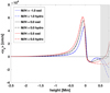 |
Fig. 4 Horizontally and time averaged vertical velocity for different metallicity values. The grey shaded area is as defined in Fig. 1. |
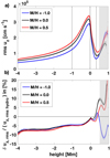 |
Fig. 5 Root mean square vertical velocities for different metallicity values. a) Root mean square vertical velocities, uz,rms, for the SSD run and b) the deviation between the SSD and the hydro run for different metallicity values. The grey shaded area is as defined in Fig. 1. The vertical lines denote heights at which the velocity distribution is obtained. |
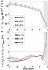 |
Fig. 6 Vertical momentum (top panel) for different M/H and ratio of vertical momentum in the SSD to the hydro simulation (bottom panel). The grey shaded area is as defined in Fig. 1. |
3.4 Magnetic fields from SSD
Small-scale turbulent magnetic fields are observed in the vicinity of the optical surface on the Sun. These magnetic fields could be explained by SSD action in the upper convection zone (Schüssler & Vögler 2008; Rempel 2014). While the small-scale turbulent magnetic fields generated by a SSD were studied for the solar case, here our aim is to investigate how these magnetic fields are affected by the metallicity of a star.
We first focus on analysing the mean absolute vertical magnetic field strength as a function of geometrical height, shown in Fig. 10. It becomes evident that in the upper convection zone, the vertical magnetic field strength is on average significantly higher in the M/H = −1.0 run than in the solar and the M/H = 0.5 run. This is expected since the magnetic field generation occurs due to the turbulent motion in the convective layers. Thus, stronger magnetic fields for the M/H = −1 metallicity are expected due to the increase in kinetic energy with decreasing metallicity (see Fig. B.1 and a discussion on the efficiency in Appendix C).
Magnetic fields generated in the convective zone emerge at the surface and are transported upwards. Therefore, closer to the optical surface there is a steep drop in the averaged magnetic field strength leading to similar mean absolute vertical magnetic field strength values at the optical surface for all three metallicities that we consider. For the solar metallicity, the mean value of the absolute vertical magnetic field at the optical surface of 71G agrees very well with previous theoretical work (Rempel 2014, 2018; Khomenko et al. 2017) and with observations (Trujillo Bueno et al. 2004; Danilovic et al. 2010; Sánchez Almeida & Martínez González 2011; Shapiro et al. 2011). A slightly higher mean absolute magnetic field of 85G is present for M/H = −1.0 and a slightly lower one of 64G for M/H = 0.5. Interestingly, a strong gradient of the field in the photosphere might be an important factor contributing to the large spread of magnetic field values determined using the Hanle effect analysis of different spectral lines (see e.g. Kleint et al. 2011; Milic & Faurobert 2012, and references therein).
Focusing on the anisotropy of magnetic fields, shown in Fig. 10b, we find that below the surface the magnetic fields are almost isotropic (independently of the metallicity). On the contrary, above the optical surface predominant horizontal magnetic fields are present and the anisotropy of the magnetic fields shows a dependence on the metallicity. Our findings for solar metallicity are consistent with those of Schüssler & Vögler (2008), who also showed that an SSD leads to predominantly horizontal fields in the solar middle photosphere.
The layers above and at the optical surface are of particular interest as most observational techniques measure the magnetic field strength at different heights above the optical surface. Thus, we show the distribution of the vertical magnetic field strength in three layers, where two of them are above the optical surface and the third is at the optical surface.
At the optical surface not only does the mean value of the absolute vertical magnetic field decrease with metallicity (see Fig. 10), but also the area covered by the concentrations of relatively strong field (see the tails of distributions plotted in Fig. 11a). Furthermore, at the surface the maximum values reached are significantly different for the three metallicities ranging from roughly 1800 G for M/H = 0.5 to roughly 2500 G for M/H = −1.0.
At about 170 km above the surface, shown in Fig. 11b, the distribution of the vertical magnetic field shows a weaker metallicity dependence compared to the optical surface (the mean absolute vertical field is roughly the same for all three metallicities). In general a flatter and wider distribution occurs with decreasing metallicity. Except for M/H = −1.0 further up at 340 km above the optical surface (see Fig. 11c), where a significantly different distribution is present.
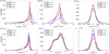 |
Fig. 7 Histograms of vertical momentum density (top panels) and vertical velocity (bottom panels) obtained in SSD simulations. The left column is at 1 Mm below the optical surface, the middle column shows the distributions at the optical surface, and the right column at about 300 km above the optical surface. |
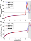 |
Fig. 8 Ratio of horizontally averaged rms horizontal to rms vertical velocity with different metallicity in (a). The grey dotted line indicates the ratio for an isotropic case. (b) The deviation of this ratio in the SSD run compared to the hydro run. The grey shaded area is as defined in Fig. 1. |
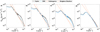 |
Fig. 9 Kinetic energy power spectra for four layers at different heights for the SSD and hydro runs with metallicity M/H = 0.0. The Kolmogorov and the Bolgiano-Obukhov scaling is also plotted, (a) At −2.5 Mm below the optical surface, (b) at −1.5 Mm below the optical surface, (c) at −0.5 Mm below the optical surface, (d) at the optical surface. |
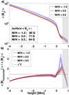 |
Fig. 10 Vertical magnetic field (a) and ratio of horizontal to vertical magnetic field (b) for the SSD simulation. The grey shaded area is as defined in Fig. 1. |
3.5 Effect of metallicity on surface structure
To illustrate the effect of metallicity on the surface structure, Fig. 12 shows example 2D plots of the vertical magnetic field, the vertical velocity at the optical surface, and the bolometric intensity at disc centre. The structure of the vertical magnetic fields look very similar for the three metallicities. This is not surprising, as Fig. 10 shows that the strengths of the vertical fields on average are very close to each other for the three metallicities around the optical surface. For the vertical velocities stronger up- and down-flows occur for the solar metallicity, but no clear trend can be identified from the snapshots. Finally, the bolometric intensity clearly shows that the intensity contrasts between inter granule lanes and granules are different. More small-scale structures become visible for M/H = −1.0. Moreover, the most prominent bright points are present in the M/H = 0.5 run. This shows that the effect of metallicity on the radiative transfer is complex and requires detailed calculations.
4 Summary and discussion
The solar surface, even in its quietest state, is covered by small-scale turbulent magnetic fields of mixed polarity (Khomenko et al. 2003; Berdyugina & Fluri 2004; Trujillo Bueno et al. 2004; Lites & Socas-Navarro 2004; Stenflo 2013), which could be explained by a SSD driven by near-surface convection (Vögler & Schüssler 2007; Schüssler & Vögler 2008; Rempel 2014). To date, SSD simulations have focused on the Sun and have achieved good agreement with observations (Danilovic et al. 2010, 2016). However, SSD simulations are lacking for other cool stars. Here we simulated for the first time the action of SSD in stars with non-solar metallicity values and investigated the effect of metallicity on the stratification, convection, and magnetic field generation and distribution in SSD simulations.
Our findings for the stratification and convection characteristics for purely hydrodynamic calculations are in agreement with previous studies (e.g. by Magic et al. 2013). The SSD calculations show similar trends with metallicity, but at the same time differ noticeably from the pure hydrodynamic calculations. In particular, momentum transport significantly changes for the SSD run in comparison with pure hydrodynamic simulations and furthermore depend on metallicity throughout the convection zone and in the lower photosphere. Moreover, the vertical velocities differ noticeably in the lower photosphere with metallicity.
Moreover, we showed that the magnetic fields generated by a SSD operating in stars of different metallicity have different properties. Generally, low metallicity stars show vertical magnetic fields of greater strength compared to stars with higher metallicity. In addition, the ratio of vertical to horizontal magnetic field strength in the photosphere changes with metallicity. The differences found in stratification and velocities are expected to affect observable quantities, such as overall spectral emission, contrasts of granules, the centre-to-limb variations, and line profiles.
So far we have analysed the intrinsic properties of the 3D simulations, where this study focused on different metallicities for solar effective temperature. A separate study investigated different spectral types (F3V, G2V, K0V, and M0V Bhatia et al. 2022). However, most of the quantities calculated in 3D simulations cannot be observed directly, even on the Sun. To understand how metallicity and small-scale turbulent magnetic fields affect observable quantities, comprehensive radiative transfer calculations are needed. Such calculations, using the MPS-ATLAS code (Witzke et al. 2021), are currently on the way and will be presented in the forthcoming publication.
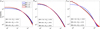 |
Fig. 11 Histogram of vertical magnetic field strength, |Bz|, distribution for three layers: (a) at the optical surface, (b) at 170 km above the optical surface, and (c) 340 km above the optical surface. |
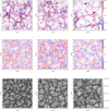 |
Fig. 12 Vertical magnetic field, Bz, vertical velocity, uz, at τ500 = 1, and bolometric intensity at disc centre for different metallicity values (from left to right M/H = −1.0, M/H = 0.0, M/H = 0.5). Top panels: Bz in units of [G]. Middle panels: uz in units of [km s−1]. Bottom panel: bolometric intensity in units of [erg cm−2 s−1]. |
Acknowledgements
This work has received funding from the European Research Council (ERC) under the European Union’s Horizon 2020 research and innovation programme (grant agreement No. 715947 and grant agreement No. 695075). We gratefully acknowledge the computational resources provided by the Cobra and Raven supercomputer systems of the Max Planck Computing and Data Facility (MPCDF) in Garching, Germany. We would like to thank A. Irwin (Free-EoS) for the open-source software used in this work.
Appendix A Stratification
Metallicity directly affects the density, and thus the pressure of the simulated plasma. Thus, another useful scale to illustrate the change in stratification is the pressure. For that we calculate the horizontally and time averaged pressure, p(z), and normalise it by the pressure value at the optical surface p(z = 0). The averages are taken at the same geometrical heights (not on iso-pressure surfaces). Figure A.1 shows the temperature structures and the temperature gradients with respect to pressure for different metallicity values.
The temperature gradient, shown in Fig. A.1 b, is smaller (at almost all heights) for lower metallicities so that lower metal-licity allows for more efficient radiative transfer, and thus for a more efficient energy transport. A local maximum in the temperature gradient close to the optical surface occurs for all three metallicities. This maximum indicates the threshold where radiative transfer becomes more efficient compared to the convective transport of energy. We note that the significantly different temperature gradients affect the radiative transfer differently for different frequency ranges of the spectra, leading to different spectral distributions of emitted radiation.
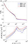 |
Fig. A.1 Horizontally and time averaged temperature structure and gradient for the SSD simulations vs pressure for different metallicity values: a) temperature, b) gradient of temperature with respect to pressure. |
Appendix B Energy spectra and typical length scale
The kinetic energy power spectra are obtained by calculating
 (B.1)
(B.1)
where  , the indicates a Fourier transform, the* indicates a complex conjugation, u is the 3D velocity field, and z denotes the vertical height of the layer.
Figure B.1 shows the kinetic energy power spectra for different layers in the SSD run with solar metallicity. The calculated power spectra are averaged in these five layers with time over at least 30 cubes, which corresponds to at least ten hours of stellar time. The overall kinetic energy in the layers decreases with height, which is expected as the density changes by several orders of magnitude between the bottom and surface of the simulated region. Moreover, the slope of the power spectra changes. It becomes steeper for wavenumbers smaller than 5 × 10⁻⁷cm−2 (which corresponds to a length scale larger than 1250 km).
In Fig. B.2 for each of the first four layers the kinetic energy spectra are shown with different metallicity. It becomes evident that while the overall kinetic energy is smallest for the M/H = 0.5 the distribution of the kinetic energy over the length scales is not significantly affected.
Finally, to estimate a typical turbulence length scale, we assume that the turbulence in the horizontal direction is isotropic and employ the integral length scale formulation
 (B.2)
(B.2)
This quantity is associated with the size of the turbulent eddies that have most of the energy (Batchelor & Press 1953). It can also interpreted as the sizes of the most predominant the convective cells. For the analysis we calculate ltyp at each layer in the simulated domain, but take the temporal average over the whole ten hours.
Figure B.3 shows the change in ltyp throughout the domain for different metallicity values. This typical integral length scale is affected by the metallicity value of the simulation at the optical surface and in the convective region (see Fig. B.3). With increasing metallicity ltyp increases around the optical surface, which can be associated with larger granules. In addition, metallicity values that are greater and lower than the solar metallicity value lead to slightly greater convection cells. This result is in agreement with previous studies of pure hydrodynamic convection with different metallicity (Magic et al. 2013).
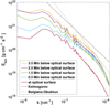 |
Fig. B.1 Kinetic energy power spectra at different heights for the SSD case with M/H = 0.0. The Kolmogorov and the Bolgiano-Obukhov scaling are also plotted. |
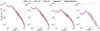 |
Fig. B.2 Kinetic energy power spectra at different heights for different metallicity values of the SSD simulation. The Kolmogorov and the Bolgiano-Obukhov scaling are also plotted: a) layer at -2.5Mm below the optical surface, b) at -1.5 Mm below the optical surface, c) at -0.5 Mm below the optical surface, d) layer at the optical surface. |
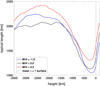 |
Fig. B.3 Typical integral length scale, as defined in equation (B.2) with height. |
Appendix C Kinetic and magnetic energies
The ratio of magnetic to kinetic energy, shown in Fig. C.1, suggests that in the deep layers an almost equipartition of the energies is reached. There is a noticeable difference with metal-licity, where the ratio is greater for higher metallicity values. While such a ratio can inform about the current state of the SSD simulation, it has no information about how much kinetic energy is potentially converted into magnetic energy.
Therefore, to understand the efficiency of the SSD we calculate the ratio of the change in kinetic energy from the hydro to the SSD run (ΔEkin = Ekin,HD − Ekin,SSD) compared to the amount of magnetic energy in the SSD simulation. Figure C.2 shows that overall this ratio is slightly above unity at the bottom of our simulation and drops below unity roughly above 2 Mm. In the upper convection zone up to 2 Mm below the optical surface the magnetic field generation or maintenance is most efficient for M/H = 0.5, while the solar metallicity is the least efficient. However, due to the complex behaviour with depth, we conclude that the generation of small-scale magnetic fields is similarly efficient for all three metallicities. The significantly stronger magnetic fields for lower metallicities are mostly due to the higher kinetic energy in these cases.
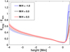 |
Fig. C.1 Ratio of magnetic energy to kinetic energy in the SSD simulations. |
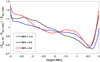 |
Fig. C.2 Ratio of magnetic energy to kinetic energy change from hydro to SSD. |
References
- Aigrain, S., Favata, F., & Gilmore, G. 2004, A&A, 414, 1139 [NASA ADS] [CrossRef] [EDP Sciences] [Google Scholar]
- Asplund, M., Grevesse, N., Sauval, A. J., & Scott, P. 2009, ARA&A, 47, 481 [NASA ADS] [CrossRef] [Google Scholar]
- Batchelor, G., & Press, C. U. 1953, The Theory of Homogeneous Turbulence, Cambridge Science Classics (Cambridge: Cambridge University Press) [Google Scholar]
- Beeck, B., Cameron, R. H., Reiners, A., & Schüssler, M. 2013, A&A, 558, A48 [NASA ADS] [CrossRef] [EDP Sciences] [Google Scholar]
- Bellot Rubio, L., & Orozco Suárez, D. 2019, Liv. Rev. Sol. Phys., 16, 1 [Google Scholar]
- Berdyugina, S. V., & Fluri, D. M. 2004, A&A, 417, 775 [NASA ADS] [CrossRef] [EDP Sciences] [Google Scholar]
- Bhatia, T. S., Cameron, R. H., Solanki, S. K., et al. 2022, A&A, 663, A166 [NASA ADS] [CrossRef] [EDP Sciences] [Google Scholar]
- Boris, J. P. 1970, NRL Memorandum Report 2167 [Google Scholar]
- Borrero, J. M., Jafarzadeh, S., Schüssler, M., & Solanki, S. K. 2017, Space Sci. Rev., 210, 275 [Google Scholar]
- Buehler, D., Lagg, A., & Solanki, S. K. 2013, A&A, 555, A33 [NASA ADS] [CrossRef] [EDP Sciences] [Google Scholar]
- Castelli, F., & Kurucz, R. L. 2003, IAU Symp., 210, A20 [Google Scholar]
- Charbonneau, P. 2020, Liv. Rev. Sol. Phys., 17, 4 [Google Scholar]
- Danilovic, S., Schüssler, M., & Solanki, S. K. 2010, A&A, 513, A1 [NASA ADS] [CrossRef] [EDP Sciences] [Google Scholar]
- Danilovic, S., Rempel, M., van Noort, M., & Cameron, R. 2016, A&A, 594, A103 [NASA ADS] [CrossRef] [EDP Sciences] [Google Scholar]
- Dedner, A., Kemm, F., Kröner, D., et al. 2002, J. Comput. Phys., 175, 645 [Google Scholar]
- Fischer, D. A., Anglada-Escude, G., Arriagada, P., et al. 2016, PASP, 128, 066001 [Google Scholar]
- Gombosi, T. I., Tóth, G., De Zeeuw, D. L., et al. 2002, J. Comput. Phys., 177, 176 [NASA ADS] [CrossRef] [Google Scholar]
- Gustafsson, B., Edvardsson, B., Eriksson, K., et al. 2008, A&A, 486, 951 [NASA ADS] [CrossRef] [EDP Sciences] [Google Scholar]
- Hotta, H., Rempel, M., & Yokoyama, T. 2015, ApJ, 803, 42 [NASA ADS] [CrossRef] [Google Scholar]
- Husser, T. O., Wende-von Berg, S., Dreizler, S., et al. 2013, A&A, 553, A6 [NASA ADS] [CrossRef] [EDP Sciences] [Google Scholar]
- Irwin, A. W. 2012, Astrophysics Source Code Library [record ascl:1211.002] [Google Scholar]
- Johnson, L. J., Norris, C. M., Unruh, Y. C., et al. 2021, MNRAS, 504, 4751 [NASA ADS] [CrossRef] [Google Scholar]
- Kaplan-Lipkin, A., Macintosh, B., Madurowicz, A., et al. 2021, AJ, 163, 205 [Google Scholar]
- Khomenko, E. V., Collados, M., Solanki, S. K., Lagg, A., & Trujillo Bueno, J. 2003, A&A, 408, 1115 [NASA ADS] [CrossRef] [EDP Sciences] [Google Scholar]
- Khomenko, E., Vitas, N., Collados, M., & de Vicente, A. 2017, A&A, 604, A66 [NASA ADS] [CrossRef] [EDP Sciences] [Google Scholar]
- Kleint, L., Shapiro, A. I., Berdyugina, S. V., & Bianda, M. 2011, A&A, 536, A47 [NASA ADS] [CrossRef] [EDP Sciences] [Google Scholar]
- Lites, B. W., & Socas-Navarro, H. 2004, ApJ, 613, 600 [NASA ADS] [CrossRef] [Google Scholar]
- Lites, B. W., Centeno, R., & McIntosh, S. W. 2014, PASJ, 66, S4 [Google Scholar]
- Livingston, W. C., & Harvey, J. 1975, BAAS, 7, 346 [NASA ADS] [Google Scholar]
- Ludwig, H. G., Caffau, E., Steffen, M., et al. 2009, Mem. Soc. Astron. Ital., 80, 711 [Google Scholar]
- Magic, Z., Collet, R., Asplund, M., et al. 2013, A&A, 557, A26 [NASA ADS] [CrossRef] [EDP Sciences] [Google Scholar]
- Magic, Z., Chiavassa, A., Collet, R., & Asplund, M. 2015, A&A, 573, A90 [NASA ADS] [CrossRef] [EDP Sciences] [Google Scholar]
- Meunier, N., & Lagrange, A. M. 2019, A&A, 628, A125 [NASA ADS] [CrossRef] [EDP Sciences] [Google Scholar]
- Meunier, N., Lagrange, A. M., & Borgniet, S. 2020, A&A, 644, A77 [NASA ADS] [CrossRef] [EDP Sciences] [Google Scholar]
- Milic, I., & Faurobert, M. 2012, A&A, 547, A38 [NASA ADS] [CrossRef] [EDP Sciences] [Google Scholar]
- Nordlund, A. 1982, A&A, 107, 1 [Google Scholar]
- Paxton, B., Bildsten, L., Dotter, A., et al. 2011, ApJS, 192, 3 [Google Scholar]
- Rackham, B. V., Apai, D., & Giampapa, M. S. 2018, ApJ, 853, 122 [Google Scholar]
- Rackham, B. V., Apai, D., & Giampapa, M. S. 2019, AJ, 157, 96 [Google Scholar]
- Rempel, M. 2014, ApJ, 789, 132 [Google Scholar]
- Rempel, M. 2016, ApJ, 834, 10 [NASA ADS] [CrossRef] [Google Scholar]
- Rempel, M. 2018, ApJ, 859, 161 [Google Scholar]
- Rempel, M. 2020, ApJ, 894, 140 [NASA ADS] [CrossRef] [Google Scholar]
- Sánchez Almeida, J., & Martínez González, M. 2011, ASP Conf. Ser., 437, 451 [Google Scholar]
- Schrijver, C. J., & Zwaan, C. 2000, Cambridge Astrophysics Series (Cambridge: Cambridge University Press), 34 [Google Scholar]
- Schüssler, M., & Vögler, A. 2008, A&A, 481, L5 [NASA ADS] [CrossRef] [EDP Sciences] [Google Scholar]
- Shapiro, A. I., Fluri, D. M., Berdyugina, S. V., Bianda, M., & Ramelli, R. 2011, A&A, 529, A139 [NASA ADS] [CrossRef] [EDP Sciences] [Google Scholar]
- Solanki, S. K., Inhester, B., & Schüssler, M. 2006, Rep. Prog. Phys., 69, 563 [Google Scholar]
- Solanki, S. K., Krivova, N. A., & Haigh, J. D. 2013, Ann. Rev. Astron. Astrophys., 51, 311 [CrossRef] [Google Scholar]
- Sowmya, K., Nèmec, N. E., Shapiro, A. I., et al. 2021, ApJ, 919, 94 [NASA ADS] [CrossRef] [Google Scholar]
- Stenflo, J. O. 2013, A&ARv, 21, 66 [NASA ADS] [CrossRef] [Google Scholar]
- Trujillo Bueno, J., Shchukina, N., & Asensio Ramos, A. 2004, Nature, 430, 326 [Google Scholar]
- Vögler, A., & Schüssler, M. 2007, A&A, 465, L43 [Google Scholar]
- Vögler, A., Bruls, J. H. M. J., & Schüssler, M. 2004, A&A, 421, 741 [NASA ADS] [CrossRef] [EDP Sciences] [Google Scholar]
- Vögler, A., Shelyag, S., Schüssler, M., et al. 2005, A&A, 429, 335 [Google Scholar]
- Witzke, V., Shapiro, A. I., Cernetic, M., et al. 2021, A&A, 653, A65 [NASA ADS] [CrossRef] [EDP Sciences] [Google Scholar]
- Yeo, K. L., Solanki, S. K., Krivova, N. A., et al. 2020, Geophys. Res. Lett., 47, e90243 [NASA ADS] [CrossRef] [Google Scholar]
All Tables
All Figures
|
Fig. 1 Horizontally and time averaged temperature structure of the SSD runs with height for different metallicity values. The grey shaded area shows the region that might be affected by the top boundary conditions (see detailed discussion in Sect. 2.3). |
| In the text | |
|
Fig. 2 Deviations in stratification from a pure hydro run to a SSD run: (a) temperature deviations; (b) density deviations; (c) pressure deviations. The grey shaded area is as defined in Fig. 1. |
| In the text | |
|
Fig. 3 Horizontally and time averaged entropy with height for the SSD simulations. The mean optical surface for all three runs is at z = 0. The vertical dash-dotted lines indicate the position of the local entropy minima. |
| In the text | |
|
Fig. 4 Horizontally and time averaged vertical velocity for different metallicity values. The grey shaded area is as defined in Fig. 1. |
| In the text | |
|
Fig. 5 Root mean square vertical velocities for different metallicity values. a) Root mean square vertical velocities, uz,rms, for the SSD run and b) the deviation between the SSD and the hydro run for different metallicity values. The grey shaded area is as defined in Fig. 1. The vertical lines denote heights at which the velocity distribution is obtained. |
| In the text | |
|
Fig. 6 Vertical momentum (top panel) for different M/H and ratio of vertical momentum in the SSD to the hydro simulation (bottom panel). The grey shaded area is as defined in Fig. 1. |
| In the text | |
|
Fig. 7 Histograms of vertical momentum density (top panels) and vertical velocity (bottom panels) obtained in SSD simulations. The left column is at 1 Mm below the optical surface, the middle column shows the distributions at the optical surface, and the right column at about 300 km above the optical surface. |
| In the text | |
|
Fig. 8 Ratio of horizontally averaged rms horizontal to rms vertical velocity with different metallicity in (a). The grey dotted line indicates the ratio for an isotropic case. (b) The deviation of this ratio in the SSD run compared to the hydro run. The grey shaded area is as defined in Fig. 1. |
| In the text | |
|
Fig. 9 Kinetic energy power spectra for four layers at different heights for the SSD and hydro runs with metallicity M/H = 0.0. The Kolmogorov and the Bolgiano-Obukhov scaling is also plotted, (a) At −2.5 Mm below the optical surface, (b) at −1.5 Mm below the optical surface, (c) at −0.5 Mm below the optical surface, (d) at the optical surface. |
| In the text | |
|
Fig. 10 Vertical magnetic field (a) and ratio of horizontal to vertical magnetic field (b) for the SSD simulation. The grey shaded area is as defined in Fig. 1. |
| In the text | |
|
Fig. 11 Histogram of vertical magnetic field strength, |Bz|, distribution for three layers: (a) at the optical surface, (b) at 170 km above the optical surface, and (c) 340 km above the optical surface. |
| In the text | |
|
Fig. 12 Vertical magnetic field, Bz, vertical velocity, uz, at τ500 = 1, and bolometric intensity at disc centre for different metallicity values (from left to right M/H = −1.0, M/H = 0.0, M/H = 0.5). Top panels: Bz in units of [G]. Middle panels: uz in units of [km s−1]. Bottom panel: bolometric intensity in units of [erg cm−2 s−1]. |
| In the text | |
|
Fig. A.1 Horizontally and time averaged temperature structure and gradient for the SSD simulations vs pressure for different metallicity values: a) temperature, b) gradient of temperature with respect to pressure. |
| In the text | |
|
Fig. B.1 Kinetic energy power spectra at different heights for the SSD case with M/H = 0.0. The Kolmogorov and the Bolgiano-Obukhov scaling are also plotted. |
| In the text | |
|
Fig. B.2 Kinetic energy power spectra at different heights for different metallicity values of the SSD simulation. The Kolmogorov and the Bolgiano-Obukhov scaling are also plotted: a) layer at -2.5Mm below the optical surface, b) at -1.5 Mm below the optical surface, c) at -0.5 Mm below the optical surface, d) layer at the optical surface. |
| In the text | |
|
Fig. B.3 Typical integral length scale, as defined in equation (B.2) with height. |
| In the text | |
|
Fig. C.1 Ratio of magnetic energy to kinetic energy in the SSD simulations. |
| In the text | |
|
Fig. C.2 Ratio of magnetic energy to kinetic energy change from hydro to SSD. |
| In the text | |
Current usage metrics show cumulative count of Article Views (full-text article views including HTML views, PDF and ePub downloads, according to the available data) and Abstracts Views on Vision4Press platform.
Data correspond to usage on the plateform after 2015. The current usage metrics is available 48-96 hours after online publication and is updated daily on week days.
Initial download of the metrics may take a while.