| Issue |
A&A
Volume 669, January 2023
|
|
|---|---|---|
| Article Number | A58 | |
| Number of page(s) | 11 | |
| Section | The Sun and the Heliosphere | |
| DOI | https://doi.org/10.1051/0004-6361/202244363 | |
| Published online | 05 January 2023 | |
The effect of shock wave properties on the release timings of solar energetic particles
1
IRAP, Université Toulouse III – Paul Sabatier, CNRS, CNES, 9th avenue du Colonel Roche BP 44346, 31028 Toulouse, France
e-mail: athkouloumvakos@gmail.com
2
The Johns Hopkins University Applied Physics Laboratory, 11101 Johns Hopkins Road, Laurel, MD 20723, USA
3
Department of Physics and Astronomy, University of Turku, 20014 Turku, Finland
4
Department of Physics, University of Helsinki, PO Box 64 00014 Helsinki, Finland
Received:
27
June
2022
Accepted:
2
October
2022
Context. Fast and wide coronal mass ejections (CMEs) and CME-driven shock waves are capable of accelerating solar energetic particles (SEPs) and releasing them in very distant locations in the solar corona and near-Sun interplanetary space. SEP events have a variety of characteristics in their release times and particle anisotropies. In some events, specifics of the SEP release times are thought to be difficult to reconcile with the scenario that a propagating shock wave is responsible for the SEP release.
Aims. Despite the apparent difficulties posed by the shock scenario, many studies have not considered the properties of the propagating shock waves when making a connection with SEP release. This could probably resolve some of the issues and would help us to delve into and understand more important issues such as the effect of the shock acceleration efficiency on the observed characteristics of the SEP timings and the role of particle transport. This study aims to approach these issues from the shock wave perspective and elucidate some of these aspects.
Methods. We constructed a simple 2D geometrical model to describe the propagation and longitudinal extension of a disturbance. We used this model to examine the longitudinal extension of the wave front from the eruption site as a function of time, to calculate the connection times as a function of the longitudinal separation angle, and to determine the shock parameters at any connection point. We examined how the kinematic and geometric properties of the disturbance could affect the timings of the SEP releases at different heliolongitudes.
Results. We show that the extension of a wave close to the solar surface may not always indicate when a magnetic connection is established for the first time. The first connection times depend on both the kinematics and geometry of the propagating wave. A shock-related SEP release process can produce a large event-to-event variation in the relationship between the connection and release times and the separation angle to the eruption site. The evolution of the shock geometry and shock strength at the field lines connected to an observer are important parameters for the observed characteristic of the release times.
Key words: Sun: coronal mass ejections (CMEs) / Sun: particle emission
© The Authors 2023
 Open Access article, published by EDP Sciences, under the terms of the Creative Commons Attribution License (https://creativecommons.org/licenses/by/4.0), which permits unrestricted use, distribution, and reproduction in any medium, provided the original work is properly cited.
This article is published in open access under the Subscribe-to-Open model. Subscribe to A&A to support open access publication.
1. Introduction
Flare- and shock-related processes are two of the main candidates for the efficient acceleration of solar energetic particles (SEPs) observed in situ (see e.g. reviews by Desai & Giacalone 2016; Klein & Dalla 2017; Vlahos et al. 2019). Solar energetic particle events are transient enhancements of the particle intensities at energies far above the typical coronal and solar wind values. Electrons with energies above a few keV to a few MeV, and protons and ions with energies from a few hundred keV to a few GeV, can be measured by energetic particle detectors on board spacecraft. These SEPs can pose a serious threat to modern technological systems on spacecraft and, most importantly, to humans in space.
For the SEPs to be observed in situ, the accelerated particles need to be injected or transported to the magnetic field lines connected to the spacecraft, regardless of the process involved in the acceleration of the particles. In this respect, fast and wide coronal mass ejections (CMEs) are powerful drivers of shock waves in the corona and interplanetary space that in turn can efficiently accelerate particles to high energies and release them in very distant locations from the flare or eruption site (e.g. Rouillard et al. 2016; Afanasiev et al. 2018; Kouloumvakos et al. 2019, 2022a). Additionally, the diffusion of SEPs perpendicular to the magnetic field lines could also be responsible for the wide distribution of SEPs (e.g. Dalla et al. 2003; Dröge et al. 2010; Laitinen et al. 2013), or this could be due to a combination of multiple processes, including the CME, the shock wave, and SEP transport effects (e.g. Rodríguez-García et al. 2021).
Multi-point observations of SEP events, for more than a decade, have made it possible to study the spatial distribution of SEPs in better detail than single-point near-Earth observations (see, e.g. Kouloumvakos et al. 2016; Lario et al. 2016). The spatial distribution of SEPs, observed near 1 au, seems to be influenced by the size of the acceleration region. Shock waves can extend widely in the solar corona (Kwon & Vourlidas 2017) and can also contribute to the wide distribution of SEPs (Kouloumvakos et al. 2022a). However, this is not the case for all the events (Rodríguez-García et al. 2021). The existence of SEP events that fill all the heliosphere, even at distant locations where the shock is thought to be difficult to reach, is a challenging issue. Additionally, there are differences in the longitudinal spread between the different species that presumably pose a challenge to the shock scenario.
Solar energetic particle events can have a variety of characteristics in their release times and particle anisotropies (e.g. Dresing et al. 2014). For example, the strong anisotropies observed during some widespread SEP events disfavour perpendicular transport, suggesting that the SEPs spread quickly close to the Sun (e.g. Gómez-Herrero et al. 2015), whereas, for some other widespread SEP events, the weak particle anisotropies suggest that perpendicular interplanetary diffusion was important (e.g. Dresing et al. 2012).
Connections of the SEP release times and the kinematics of the associated EUV waves show that, for some events, the energetic proton release times are associated with the shock wave arrival time to the field lines connected to the spacecraft (e.g. Park et al. 2013; Prise et al. 2014), whereas, for some other events, the release of the energetic electrons is much earlier than the connection of EUV waves to the observer (e.g. Miteva et al. 2014). This inconsistency seems to pose a challenge to the acceleration and release of the SEPs from a shock wave low in the corona. However, recent studies have shown that the geometric and kinematic properties of shock waves higher in the low corona could result in the earlier release of SEPs than the expansion properties of the EUV waves suggest (Zhu et al. 2018; Kouloumvakos et al. 2022a). The fast shock expansion at higher altitudes could be responsible for the observed SEPs’ release times in many cases.
Another aspect is the observed delays between type III emissions and the SEP onset times at different widely separated spacecraft (e.g. Richardson et al. 2014). These delays have been attributed to either the expansion properties of the acceleration region or to the time required for the particles to diffuse (Kollhoff et al. 2021). In this regard, the release of protons and electrons is shown to be simultaneous in most of the SEP events, and both species are delayed from the start of the type III emission (Kouloumvakos et al. 2015; Xie et al. 2016; Ameri et al. 2019). This seems to be the case at least for events where the location of magnetic connections to the observers is > 90° from the flare site. In these cases, it is most probable that the expanding shock waves accelerate and release SEPs to open field lines, and any observed delay in the SEP release times can be attributed, at least, to the time it takes for the acceleration region to reach the field lines connected to each spacecraft (e.g. Malandraki et al. 2009; Rouillard et al. 2012; Kouloumvakos et al. 2016).
On the other hand, in some widespread SEP events the release of energetic protons is after the energetic electrons, suggesting a late acceleration or release of the protons close to the Sun. The exact mechanism causing the delays remains unclear. The differences in the spread and release between the two species pose a challenge to the view that the expansion of an acceleration region is responsible for the release of SEPs during these events. Perpendicular transport effects are thought to be more important; however, it is not clear if the differences in the time delays can also be explained by the properties and specifics of the acceleration process from the shock wave itself.
In this study, we present a simple geometrical model to describe the propagation and longitudinal extension of a disturbance. We used the geometrical model to examine the longitudinal extension of the wave-front from the eruption site as a function of time. Then we examined how the kinematic and geometric properties of the disturbance could affect the timings of the SEP releases at different heliolongitudes. We also considered the spatiotemporal evolution of the shock geometry (ΘBn angle) and the shock strength. We examined if the changing shock properties of the field lines connected to an observer could be a possible reason for the observed timings of the SEP releases. We emphasize that the values of the various parameters used in this study can vary from event to event in reality. They are used to build our discussion, analytically and quantitatively, on the possible delays of the SEP acceleration and release times from a propagating disturbance in the corona. The final results that we present in this study should be regarded in such a context. After our discussion, we show details of a novel python software package and a web application that can be used to model, in 2D, the shock wave parameters in the corona and IP space, and to calculate the connection times at different locations.
2. The geometrical model
2.1. Overview
Coronal mass ejections can exhibit a wide range of morphologies in coronagraph observations, but the 3D shape of CME-driven shock waves is usually approximated with a spherical model. Previous studies have shown that an ellipsoid model represents very well the shape of the envelope of the waves propagating in the solar corona (e.g. Kwon & Vourlidas 2017; Liu et al. 2017); hence, we use an ellipse as a basis for our 2D model. We consider the propagation of a disturbance from a point located at the solar surface at (x, y) = (R⊙, 0). The geometrical model of the disturbance will be an ellipse in the most general case. The two semi-axes, Rx and Ry, are aligned with the x-axis and y-axis, respectively. Figure 1 shows a sketch of the geometrical model considered here. In this case, the two semi-axes are equal, so the propagating disturbance expands spherically and it is depicted with the red circles. Defining ϵ as the ratio of the length of the two semi-axes, Ry/Rx, we have that for ϵ = 1, the disturbance expands spherically, while for any other value the disturbance expands faster in one of the two directions.
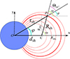 |
Fig. 1. Sketch of the geometrical model of the disturbance. The red circles depict the disturbance front location at different time steps. The blue circle represents the Sun and it is centred at the axis origin. We label the geometrical parameters we used in the model. The labels rsh and Rsh are the distance of a given point, P, located at the disturbance from the solar centre (O) and the disturbance centre (C), and φ is the ∡ COP angle, i.e. the longitudinal separation angle from the disturbance source region. |
For the propagation of the disturbance, we constructed a simple kinematic model assuming that it expands with a constant acceleration. The length of the two semi-axes as a function of time is given by the following two equations:
At t = 0 the disturbance has an initial expansion speed, V0, a constant acceleration, a0, and its centre is located at the solar surface. We also considered a propagation of the disturbance along the x-axis, which models a translation of the shock centre similar to what previous studies have shown. For example, Liu et al. (2017) were able to separate translation from expansion in the shock motion for an event and showed that the expansion of a shock, which was roughly self-similar during the event, largely dominates over the translation of the shock centre. This translation in our model equals the disturbance’s expansion kinematic profile (at the same direction) multiplied by a constant, α ∈ [0, 1). For α = 0 the centre of the disturbance is static and is always located at the solar surface, while for α > 0 the centre moves away from the Sun and is always located above the surface for t > 0, as we show in Fig. 1. The distance of the disturbance centre from the solar centre (dsh) is given by
In Fig. 2, we show the propagation of a disturbance using different parameters. In any case, we used the same expansion speed (Vexp = 800 km s−1) but different values for α and ϵ. For panels a to c, we used the same ϵ value and changed α from 0.4 to 0.8, while for panels d and e, we used the same α and changed ϵ from 0.8 to 1.2. In panel f we show the case where α = 0 and ϵ = 0. In this case, the centre of the disturbance was always located at the solar surface.
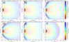 |
Fig. 2. Two views of the propagating disturbance (coloured circles) using the geometrical model at the same expansion speed (Vexp = 800 km s−1), but with two different values for the α parameter. We used α = 0.25 for the top panel and α = 0.75 for the bottom panel. The yellow circle represents the Sun and it is centred at the axis origin. At t = 0 the disturbance is located at the Sun’s surface. |
In panels a to c, we show that by increasing the α value, the disturbance propagates slower at locations below the flanks and near the solar surface, and faster at locations above the flanks and towards the apex of the disturbance. In the extreme limit where α is unity, so that the propagation speed Vp is equal to the expansion speed Vexp, all the ellipses become tangent to the solar surface. For α values greater than unity, the ellipses detach completely from the Sun and these values lead to a non-physical description of the disturbance. As shown in Liu et al. (2019) from the analysis of the very energetic event of 10 September 2017, the radial and lateral expansion speeds of the shock are larger than the translational speed of the shock centre. This is what we expect to be the case, overall, for most of the events. On the other hand, α values close to zero lead to an extension of the disturbance at the solar surface, which is very rapid and probably inconsistent with the observations. This case can be seen in the last panel of the bottom row of Fig. 2 where α = 0. Previous studies have shown that the Vp/Vexp ∼ 0.8 for wide CMEs (e.g. Gopalswamy et al. 2009). However, for propagating shock waves in the solar corona, the α values can be lower. For example, this could be the case for events where the shock wave expands rapidly away from the CME flanks and becomes the observed halo part of the CME (e.g. Kwon & Vourlidas 2017; Liu et al. 2019).
In panels d and e, we show two cases with ϵ ≠ 1. For ϵ < 1, the flanks of the disturbance expand slower than the apex, while for ϵ > 1 the flanks expand faster. In any case, when ϵ ≠ 1 the shape of the disturbance is an ellipse.
2.2. Connection times
We used the geometrical model presented in the previous section and we calculated the time that it took for the disturbance to propagate to different locations and magnetically connect to the observers. We started from the ellipse equation in the Cartesian coordinate system:
where the centre of the ellipse is at (x0, y0), and a and b are the two semi-axes, respectively. From the geometrical model of Fig. 1, the centre of the disturbance is always located on the x-axis at a point with coordinates (dsh(t),0) and the two semi-axes a and b are denoted as Rx and Ry, respectively. Thus, the ellipse equation becomes

where ϵ = Ry/Rx, as defined previously. Equation (4a) can be written in polar coordinates using (x, y) → (r cos ϕ, r sin ϕ), where ϕ is the polar (or longitudinal) angle and r is the distance from the axis origin. Thus, we have

We use this equation to calculate the time that it takes for the disturbance to propagate to a point with coordinates (rp, ϕp) and connect to an observer. First, we solve Eq. (5) for Rx(t) using also Eq. (2) for dsh(t). After some algebraic calculations, Eq. (5) becomes

where

From the above, Rx(t) can be found from the solution of the quadratic equation, which is  . Then we use Eq. (1) and solve for the connection time, so that
Using this equation we calculated the connection time of the disturbance to any point in the heliosphere.
We also used Eq. (7) to parametrize the time of connection as a function of the longitudinal separation angle ϕ. We calculated the connection times of the disturbance to the footpoints at the solar surface of the magnetic field lines and the first connection times of the disturbance to the magnetic field lines. We note that the two connection times are not the same and depend on the geometry of the disturbance, as we show later in the analysis. The connection times with the footpoints at the solar surface can be calculated as a function of ϕ using Eqs. (6a) and (7), and setting rp = R⊙. This is because all the points lie on the solar surface.
Figures 3a1–a3 show the connection time of the disturbance to the footpoints at the solar surface as a function of ϕ. For each line, we used different parameters for the geometrical model. For panel a1, we used different expansion speeds, V0, which ranged from 500 to 1500 km s−1, and constant α and ϵ. From this panel, it is obvious that higher disturbance expansion speeds lead to lower connection times, as expected. Between the two extreme values for V0 (500 and 1500 km s−1), the difference in the connection times ranged from a few minutes (∼3 min) for ϕ ∼ 10° to a few tens of minutes (∼37 min) for ϕ ∼ 90°. In panel a2, we used different values for α, which ranged from zero to one, and also used constant V0 and ϵ. Higher α values lead to later connection times. At high ϕ values, the time difference in connections becomes important, and thus, as the α values increase, the connection times are delayed to more than three hours for the extreme α values shown in panel a2, and for ϕ values close to 90°. In panel a3, we used different values for ϵ that ranged from 0.8 to 1.5, and we kept V0 and α constant. In this case, the time differences in the connection times when changing only ϵ were small and in the order of a few minutes.
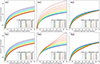 |
Fig. 3. Disturbance connection times as a function of the longitudinal separation angle from the eruption site for different model parameters. We use, in the left panels, constant α and varying expansion speed. In the middle panels, we use constant expansion speed and varying α. In the right panels, we use constant speed at the apex and varying ϵ. |
To calculate the time taken for the disturbance to connect to the magnetic field lines for the first time, we have to find where and when the field lines and the ellipse become tangent. To make the calculation easier, in this step we assume that the field lines in the low corona can be approximated as straight lines. This is a good approximation for Parker spirals at a height between 1 and 20 R⊙ where the first connections have already been established. However, this is a zeroth-order approximation. Even when a current free (potential) field is assumed for the corona, the magnetic field lines below the solar source surface radius, at which the coronal magnetic field is considered to be radial and is usually assumed to be at 2.5 R⊙ from the Sun’s centre, can be very complex.
Therefore, starting from the equation of an ellipse in Cartesian coordinates,  , and the equation of line y = mx, we calculated where the line is tangent to the ellipse by solving the cubic equation for x and calculating the Rx by setting the discriminant equal to zero. The line is tangent at a point with coordinates xt = −b/(2a) and yt = mx = −mb/(2a). The time of the first connection to the field lines can be calculated from Eq. (7), and using
  and ϕp = arctan2(yt, xt) to calculate the coefficients of Eq. (6b).
In Figs. 3b1–b3, we show the first connection times of the disturbance to the field lines as a function of ϕ, similar to what we presented for the top row panels and using different parameters for the geometrical model. Comparing the top with the bottom row panels, we see that the connection time of the disturbance to the footpoints at the solar surface may not be the first time that the disturbance connects to the field lines. This is a geometrical effect of the disturbance model primarily coming from the α parameter. For α = 0 the first connections for all ϕs are established at the solar surface, while for α > 0, the first connections can be located above the solar surface and be earlier than the connection at the footpoints at the solar surface. This time difference becomes more important for increasing α values.
From panel b1, we see that with increasing V0, the difference at the connection times ranges from a few minutes for ϕ ∼ 10° to a few tens of minutes for ϕ ∼ 90°, similar to what we show in panel a1. From panel b2, comparing the time differences between the extreme α values used, we see that for ϕ ∼ 10° the time differences in connections are in the order of seconds, while for ϕ ∼ 90° they are in the order of hours. For panel b3, the results are similar to those presented for panel a3. The differences in connection times are in the order of a few minutes between the extreme ϵ values.
2.3. Calculating the shock geometry
At the next step of this analysis, we used the geometrical model to calculate the ΘBn angle, which is as the magnetic field obliquity with respect to the disturbance or shock front normal direction. In Fig. 4, we show a sketch of the disturbance and the vectors that define the different directions and the angles needed to calculate the ΘBn angle. The ΘBn at a point of connection P is
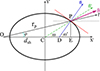 |
Fig. 4. Sketch of the geometrical model of the disturbance employed in the current study that shows the different points, angles, and vectors that we define in the text and are needed to calculate the ΘBn angle. |
where Θrn is the angle between the position vector, rsh, and the disturbance and shock front normal vector, and ΘBr is the angle between rsh and the magnetic field vector.
First, we calculated the Θrn angle at the point of connection, P, (see Fig. 4). For ϵ ≠ 0 the disturbance is an ellipse and we have

where ω′ is the ∡ PDE angle in Fig. 4, so tanω′ is the slope of the normal line DP to the ellipse. There is a relationship between ω′, ω, and ϵ, which can be shown by starting from the standard equation of the ellipse and taking the derivative with respect to x, which gives us the slope of a line tangent to the ellipse at a point (x, y). So the derivative of Eq. (3) is dy/dx = −(Ry/Rx)2(x/y). The slope of the normal line is the negative reciprocal of this, so tanω′= − dx/dy = (Rx/Ry)2(y/x) = ϵ−2(y/x). Since, tanω = y/x, the relation becomes
From this equation, in the simple case where ϵ = 1, the disturbance is a circle, and thus n and n′ (and the points C and D) coincide, and ω = ω′. In this case, Θrn = ω − ϕ.
The ω angle can be calculated from the two sides, PE and CE, of the OPE triangle in Fig. 1. Therefore, we have
where rp and dsh are known. Synopsising the above calculations, when ϵ ≠ 0, we calculated the ω first from Eq. (11). Then, using Eq. (10), we calculated the ω′, and lastly Θrn from Eq. (9).
The next step was to calculate the ΘBr angle. This depends on the selected magnetic model, but since we assumed that the field lines are straight lines in the low corona, the ΘBr angle in this case was zero. If we had assumed that the field lines were Parker spirals from 1 R⊙ to the observer, then in this case, the ΘBr angle would be a function of distance and the solar wind speed (Vsw) used in the spiral model (see Eq. (13.12) in Priest 2014). The calculation of ΘBr angle then becomes:
where Ω is the equatorial sidereal rotation rate of the Sun and Vsw is the solar wind speed. In the case of more realistic magnetic field models of the solar corona, such as the Potential Field Source Surface (PFSS) model, the magnetic topology becomes more complex. However, the ΘBr angle can be calculated from the dot product of the two vectors.
Figure 5 shows the connection time of the disturbance as a function of the longitudinal separation angle, similar to what we show in Fig. 3. For the different panels, we used the same expansion speed (V0 = 800 km s−1), and different α and ϵ values. The coloured contours depict the ΘBn values at different locations, and essentially they show the changing ΘBn angle as a function of time and the longitudinal separation angle. For the calculation ΘBn, we assumed that the field lines are Parker spirals and we used Eq. (12) for the calculation of ΘBr.
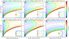 |
Fig. 5. Disturbance connection times as a function of the longitudinal separation angle from the eruption site for an expansion speed of 800 km s−1 and varying α values among the different panels. The blue curves show the times that the disturbance connects to field lines for the first time, the solid black curves show the time that the disturbance connects at the same field lines at the solar surface. The coloured curves show the connection times when the disturbance has a specific ΘBn at the connected field lines. The dashed black curves show the time when ΘBn = 45° (oblique geometry). For the calculation of ΘBn, we assumed that the field lines are Parker spirals (ΘBr ≠ 0°). The inset plot in each of the panels shows the propagating disturbance (coloured circles) for the different set of parameters used. |
From Fig. 5, we notice that the time at which the disturbance connects to the field lines for the first time (tcf) can be different to the time (tcs) that the disturbance reaches and connects to the footpoints of the field lines at the solar surface. In these cases, the disturbance connects to the field lines for the first time above the solar surface. This leads to first connections higher in the corona that occur earlier than the connections at the solar surface. Comparing the curves of tcs and tcf for the top row panels, we see that the time difference between the two curves increases with increasing α values. From Fig. 5c we find that for α ≥ 0.8, the time difference is a few minutes for ϕ ∼ 10–40°. For α = 0 (see Fig. 5f), the first connections of the disturbance and the field lines are always located at the solar surface (so tcs = tcf).
When the disturbance connects to the field lines for the first time, the front geometry is mainly oblique (ΘBn = 45°) or quasi-perpendicular (ΘBn ≫ 45°) for every ϕ, except from the very low ϕ values (e.g. ≪5°) where the shock geometry is mainly quasi-parallel (‘perpendicular’ and ‘parallel’ shock geometry refer to the orientation of the magnetic field upstream to the normal to the shock front). This is apparent in most of the panels of Fig. 5. In each panel, we show with the dash-dotted black line the time and location that the geometry is oblique. For increasing α values, the time that it takes for the ΘBn to change from a quasi-perpendicular to a quasi-parallel values also increases. This can be seen by comparing the lines for ΘBn = 45° between the different panels of Fig. 5. In particular, for ϕ much greater than 30°, this time becomes important. For example, compared to α = 0.6, we find that for α = 0.8 and ϕ = 45° the disturbance needs to expand for an additional ∼1 h along the connected field lines for the geometry to change from quasi-perpendicular to oblique. Overall, we find that even for the extreme case where α = 0.99, the time that it takes for the ΘBn to change to oblique values is ≤15 min for ϕ ≤ 30°, while for ϕ ≫ 30° this time is significantly greater (in the order of hours).
2.4. Calculating the shock strength
Using the kinematics of the modelled disturbance and coronal models of the density and the magnetic field, we can determine the evolution shock strength, quantified here from the Alfvénic Mach number, and also determine if a shock wave forms at any location along the connected magnetic field lines. The development of a shock in a magnetized plasma is characterized by the ratio between the flow speed, V′, in the shock reference frame, and the Alfvén speed, VA. The VA is a characteristic speed of the magnetized plasma that depends on the magnitude of the magnetic field and the plasma density. To calculate the VA, for simplicity we used two different broadly used density models (Newkirk 1961; Saito et al. 1977) and a magnetic model corresponding to quiet-Sun conditions.
Several coronal models have been introduced to describe the variation in electron density with the heliocentric distance. The electron density in these models is either exponential (e.g. Newkirk 1961), or more frequently, finite sums of power-law terms in heliocentric distance (e.g. Saito et al. 1977; Leblanc et al. 1998). In this study, we used the Newkirk (1961) and Saito et al. (1977) models. The one-fold Newkirk model corresponds to a barometric height model derived for a gravitationally stratified corona with a temperature of 1.4 × 10⁶ K, while, the Saito model is derived from measurements of polarized brightness in the corona. We note that the Newkirk model is hydrostatic, so it should not be used in the solar wind. It applies only if Vsw ≪ vth (i.e. if the flow is clearly subsonic). The two models have one to two orders of magnitude differences in the density above ∼10 R⊙, with the Newkirk model being denser than the Saito model. At the solar surface, the density of the one-fold Newkirk model is ∼1.9 times greater than the density of the Saito model.
Using the electron number density from the two selected models, we calculated the full particle number density as N = 1.92 Ne (using a mean molecular weight  ). The Alfvénic Mach number is defined as MA = V′/VA and
  (B in Gauss). From the dependence of the shock strength on the coronal density, we see that using a ‘dense’ coronal model gives an upper limit of the shock strength, while, a less ‘dense model’ gives a lower limit. For the coronal magnetic field strength, we used a simple model corresponding to quiet-Sun conditions (see Mann et al. 1999, 2003, for further details), where the magnitude of the magnetic field as a function of the heliocentric distance is given by B(r) = B0(R⊙/r)α0. For B0 we used a value of 2.2 Gauss, which corresponds to a typical value of the magnetic field in quiet photospheric regions, and α0 = 2. To keep the complexity of our model within a reasonable level, we did not include in the magnetic model any active-Sun component contribution, for example, a component from an active region, similar to what was considered, for example, in the Mann et al. (2003) study.
The speed of the disturbance along the normal vector direction can be calculated from the expansion and propagation speeds as  . Additionally, to calculate MA we also considered the radial variation in the solar wind speed with the distance from the centre of the Sun. This is because MA is defined in the shock reference frame,
  , where
  is the solar wind speed along the shock normal direction. To calculate υ = Vsw(r), we used Parker’s isothermal solution. In this case, υ is given implicitly from the following transcendental equation:
where  is the isothermal sound speed for a temperature T,
  is a critical point where the solar wind speed is equal to the sound speed and is a saddle point of Eq. (13), and C = −3 for the standard solution of solar wind. Following Cranmer (2004), the solution of Eq. (13) can be written explicitly from the Lambert function as
 ![$ \upsilon^2 = -\upsilon_{\rm c}^2 W_{\pm} [-D(r)] $](/articles/aa/full_html/2023/01/aa44363-22/aa44363-22-eq26.gif) , with D(r) = (r/rc)−4exp(4(1 − rc/r)−1) and using W+ for r ≤ rc and W− for r ≥ rc. Here we used a temperature of 1.4 × 10⁶ K, which gives a sound speed of ∼128 km s−1, a critical-point location at ∼5.8 R⊙, and a solar wind speed of ∼320 km s−1 at 30 R⊙.
, with D(r) = (r/rc)−4exp(4(1 − rc/r)−1) and using W+ for r ≤ rc and W− for r ≥ rc. Here we used a temperature of 1.4 × 10⁶ K, which gives a sound speed of ∼128 km s−1, a critical-point location at ∼5.8 R⊙, and a solar wind speed of ∼320 km s−1 at 30 R⊙.
In Fig. 6, we show the disturbance’s connection times as a function of the longitudinal separation angle, similar to those presented in Fig. 5. In these panels, we overlay the calculated MA values using black contours. We used the same model parameters as in Fig. 5 (e.g. V0 = 800 km s−1 and α = 0.8). For the left panel, the MA was calculated by using the Saito density model, whereas for the right panel we used the one-fold Newkirk density model. As noted earlier, the Newkirk density model is a few orders ‘denser’ than the Saito model. Therefore, the MA values shown in the left panel are overall lower estimates than those of the right panel at a given height. In both cases, we find that a shock forms quickly for separation angles lower than 45°. However, this is not the case for greater angles where the MA can be less than unity for several hours. From the results of the left panel, we see that for ϕ ≫ 45°, the shock formation from a disturbance that propagates with a speed of 800 km s−1 can be significantly delayed after the first magnetic connections have been established. In the case of the Saito model, we find that for ϕ > 70° it would take more than two hours for a shock wave to form at the magnetically connected field lines if the wave has not completely damped and there is also no influence from the CME. Liu et al. (2017, 2019) have suggested that an observed expanding disturbance can be just a propagating wave without a non-linear steepening character, especially when the driver’s influence becomes weak along certain directions and the disturbance is a freely propagating wave or a decaying shock wave that progressively dissipates into a simple wave. Overall, for high ϕ values, we find that the time that it takes for the shock wave to form decreases with increasing V0 or with decreasing α values. This happens because the shock flanks in both cases propagate faster.
 |
Fig. 6. Plots similar to those presented in Fig. 5, showing the disturbance connection times as a function of the longitudinal separation angle. Here an expansion speed of 800 km s−1 and α = 0.8 are used in both panels. The black contour lines show the evolution of MA values for different angles and times. The MA were calculated using two different coronal models for the variation in density with the heliocentric distance. For the left panel, we used the Saito model and for the right panel, we used the Newkirk model. |
Additionally, considering that shock waves accelerate particles more efficiently when they become supercritical, since in this case a significant part of upstream particles can be injected efficiently into the acceleration process, we would expect that there is an additional time delay for the onset of SEP acceleration or a release to the connected magnetic field lines. The critical Alfvénic Mach number, Mc, depends on the angle ΘBn and the plasma beta parameter. For a quasi-parallel shock geometry (ΘBn < 45°), the Mc ranges between 1.5 to 2.0, while for quasi-perpendicular shock geometry (ΘBn > 45°), the Mc is higher and ranges between 2.0 to 2.7 (see e.g. Fig. 8 in Mann et al. 2003). From Figs. 5 and 6, we see that the shock geometry changes rapidly from quasi-parallel to quasi-perpendicular in most of the cases. Additionally, for ϕ ≪ 45° the MA ≫ 1.5 (e.g. supercritical), even during the earliest stages of the shock expansion, while for ϕ ≫ 45° the shock may need additional time to become supercritical at the connected field lines. In any case, as far as the acceleration and release of SEPs from the shock wave is concerned, we find that for large longitudinal separation angles (ϕ ≪ 45°), there is probably an additional time delay after the shock formation until the shock wave starts accelerating particles efficiently. Another aspect is that the shock geometry could also have an additional effect on the acceleration efficiency of the different particle species (protons versus electrons). This is difficult to address in this analysis, but it should be expected, given the range of different shock geometry angles at the connected field lines and the rapid changes in the shock geometry that we find, even for this simple magnetic configuration we consider in this study.
An example of the evolution of the shock parameters (ΘBn, top panel and MA, bottom panel) as a function of time is given in Fig. 7. Each line in the panels depicts the evolution of the shock parameter along a specific magnetic field line whose footpoint at the solar surface has a longitudinal separation angle, Φ. We used different line colours for each field line. The evolution of ΘBn shows that at the flanks of the disturbance (e.g. Φ > 70°) there is a rapid change in the shock geometry from quasi-perpendicular to oblique. Near the apex the ΘBn starts from quasi-parallel and progressively changes into oblique. The MA also changes rapidly and it is different between the apex and the flanks.
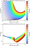 |
Fig. 7. Evolution of the shock parameters, ΘBn (top panel) and MA (bottom panel), as a function of time. |
3. Discussion and conclusions
In this study, we introduce a simple geometrical model to describe the propagation of a disturbance. We used this model to examine the connection times of a disturbance to broad heliolongitudes, and how the propagation and expansion characteristics are affecting the connection times. First, we show how different initial parameters of the modelled disturbance result in a broad range of connection times at a given longitudinal separation angle. Fast and wide disturbances reach the magnetic field lines connecting to an observer more rapidly than slow and narrow fronts, as expected. When the disturbance’s propagation speed is not zero (e.g. α ≠ 0), which is rather the case for most of the events, the regions below the flanks of the disturbance and towards the solar surface propagate slower than those above the flanks and towards the apex. In this case, we show that there is a delay in the disturbance’s connection time to the field lines compared to the case where α = 0 and this is particularly significant for separation angles greater than 45°.
We also show that the longitudinal extension of the disturbance close to the solar surface may not always be indicative of the time that a shock wave connects for the first time to the magnetic field lines connecting to the observers. When α ≫ 0 the first magnetic connections of the disturbance to the observers occur mostly at locations above the solar surface. This is because the disturbance extends faster higher in the corona than close to the solar surface. This is, for example, the case for the 27 January 2012 event, where Zhu et al. (2018) find that even though there was no obvious evidence to indicate that the EUV wave reached the magnetic footpoints of the observers, a connection to the shock was established higher in the middle corona. The time of connection was consistent with the release of the observed SEP event. This seems to be an important aspect of the observed delays between the particle release and onset times, and the times that the EUV waves connect to the magnetic field lines. A systematic analysis of a big sample of events can show further evidence that the expansion of shock waves higher in the middle corona can become more important than the EUV extension in the low corona, as far as the SEP release is concerned.
Other important characteristics that could probably lead to a significant delay in the release of the particles, after the time that the shock wave connects to the observer, are the complex temporal and spatial evolution of the shock properties, and the shock acceleration efficiency, which depend on the shock strength and geometry and are different for each species. Detailed shock modelling (e.g. Rouillard et al. 2016; Kouloumvakos et al. 2019) has shown that there is considerable variability of the shock parameters along the shock surface as the shock wave expands from the low corona into interplanetary space. The shock geometry (ΘBn), for example, can change dramatically as the shock wave evolves from the low corona into interplanetary space, while it intercepts different coronal structures during its expansion. Differences in the acceleration efficiency for electrons and protons at quasi-parallel and quasi-perpendicular shocks have been shown by previous studies, and are expected by the theory. This could be a reasonable explanation for the time delays observed between the two species, electrons and protons. If the energetic electrons are accelerated more efficiently at quasi-perpendicular shock conditions and protons are accelerated more efficiently at quasi-parallel shocks, then we would expect that the acceleration and release times for electrons could be very different from those of protons, depending on the shock geometry. In this context, we showed that for low separation angles the shock geometry changes rapidly from quasi-perpendicular to quasi-parallel, while for high separation angles the shock needs additional time to pass the oblique limit towards the quasi-parallel geometry. This is an important effect to be considered in future studies.
In addition, we have shown that the evolution of the shock strength, as well as the properties of the background medium, could also be important. Even when a disturbance is magnetically connected to an observer, this may not have steepened into a shock wave and in this case, the SEP acceleration has not yet started. It is a possibility that in some cases the propagating disturbance needs an additional time to steepen into a shock wave along the well-connected field lines to an observer, or it may never steepen into a shock at all, depending on the local coronal conditions (see the discussion in Kouloumvakos et al. 2022a). This additional time could possibly be one of the reasons that significant time delays are observed between the SEP release times and the times that the disturbances connect to the observer.
Even when a shock wave has formed, it needs to become super-critical to start accelerating particles efficiently, especially ions. This additional time that the shock wave may need to become super-critical could be another reason for the delay in the observed SEP release and onset times with respect to the shock connection times. This delay may not be the same for the two particle species since electrons can be easily reflected in shocks that have any kind of magnetic compression (i.e. quasi-perpendicular ones), even if they are sub-critical. However, this is not the same for thermal protons, since their injection in the acceleration process could be very inefficient in sub-critical shocks. Therefore, there is considerable complexity when attempting to connect the evolution of a disturbance in the corona with the observed characteristics of widespread SEP events, since the properties of the shock waves can certainly affect the release timings of solar energetic particles.
The results of this study can be summarized as follows:
-
From a shock-related SEP release process, we expect a large event-to-event variation in the relationship between the connection times and the separation angle to the eruption site, especially for distant magnetic connections.
-
The extension of a wave close to the solar surface may not always indicate accurately when a magnetic connection is established for the first time. This depends on the kinematics and geometry of the wave.
-
The evolution of the shock geometry and shock strength at the field lines connected to an observer can be important parameters for the observed delays between the SEP release and onset times, and the times when the shock waves connect to the observers.
The different aspects presented in this study should be tested in the context of the new solar observations made by the two new solar missions of the Parker Solar Probe and Solar Orbiter. The complexities may be considerable, but but shock modelling techniques are continually being improved (e.g. Kwon & Vourlidas 2017; Lario et al. 2016; Rouillard et al. 2016; Zhu et al. 2021; Kouloumvakos et al. 2019), which can be used to interpret the SEP observations of the new solar missions (see e.g. Kouloumvakos et al. 2020, 2022a). The model presented here may be simpler than the more sophisticated methods currently available, yet it can be used to analyse solar events and derive important information for the shock properties through a comprehensive process with relatively low complexity. In the future, we envision that further developments of this model will make it more sophisticated. This, for example, can be incorporated with the use of more realistic coronal and solar wind background models, such as the PFSS model or magnetohydrodynamic models. Additionally, the kinematics and the expansion parameters of the model can be more realistic, when analysing specific events, with the use of tools that perform reconstruction of the CME or shock wave 3D structure using remote-sensing observations from multiple viewpoints. For example, using PyThea1, a new Python software package that can be used to reconstruct shock waves and CMEs in 3D (Kouloumvakos et al. 2022b), the provided parameters can be more realistic. In Appendix A, we present an open-source Python software package and a web application that is developed with the hope that it will be useful to the community and for the analysis of solar events with the model.
Acknowledgments
This study has received funding from the European Union’s Horizon 2020 research and innovation programme under grant agreement No. 101004159 (SERPENTINE). A.K. acknowledges financial support from the SERPENTINE project for the tool development and from NASA NNN06AA01C (SO-SIS Phase-E) contract that allowed to complete this study. J.G. and R.V. acknowledge the support of Academy of Finland (FORESAIL, grants 312357 and 336809). D.P. acknowledges the ERC under the European Union’s Horizon 2020 research and innovation programme (Grant agreement No. 724391, SolMAG).
References
- Afanasiev, A., Vainio, R., Rouillard, A. P., et al. 2018, A&A, 614, A4 [NASA ADS] [CrossRef] [EDP Sciences] [Google Scholar]
- Ameri, D., Valtonen, E., & Pohjolainen, S. 2019, Sol. Phys., 294, 122 [NASA ADS] [CrossRef] [Google Scholar]
- Cranmer, S. R. 2004, Am. J. Phys., 72, 1397 [NASA ADS] [CrossRef] [Google Scholar]
- Dalla, S., Balogh, A., Krucker, S., et al. 2003, Geophys. Res. Lett., 30, 8035 [NASA ADS] [CrossRef] [Google Scholar]
- Desai, M., & Giacalone, J. 2016, Liv. Rev. Sol. Phys., 13, 3 [NASA ADS] [CrossRef] [Google Scholar]
- Dresing, N., Gómez-Herrero, R., Klassen, A., et al. 2012, Sol. Phys., 281, 281 [NASA ADS] [Google Scholar]
- Dresing, N., Gómez-Herrero, R., Heber, B., et al. 2014, A&A, 567, A27 [NASA ADS] [CrossRef] [EDP Sciences] [Google Scholar]
- Dröge, W., Kartavykh, Y. Y., Klecker, B., et al. 2010, ApJ, 709, 912 [CrossRef] [Google Scholar]
- Gómez-Herrero, R., Dresing, N., Klassen, A., et al. 2015, ApJ, 799, 55 [Google Scholar]
- Gopalswamy, N., Dal Lago, A., Yashiro, S., et al. 2009, Cent. Eur. Astrophys. Bull., 33, 115 [Google Scholar]
- Klein, K.-L., & Dalla, S. 2017, Space Sci. Rev., 212, 1107 [Google Scholar]
- Kollhoff, A., Kouloumvakos, A., Lario, D., et al. 2021, A&A, 656, A20 [NASA ADS] [CrossRef] [EDP Sciences] [Google Scholar]
- Kouloumvakos, A., Nindos, A., Valtonen, E., et al. 2015, A&A, 580, A80 [NASA ADS] [CrossRef] [EDP Sciences] [Google Scholar]
- Kouloumvakos, A., Patsourakos, S., Nindos, A., et al. 2016, ApJ, 821, 31 [NASA ADS] [CrossRef] [Google Scholar]
- Kouloumvakos, A., Rouillard, A. P., Wu, Y., et al. 2019, ApJ, 876, 80 [NASA ADS] [CrossRef] [Google Scholar]
- Kouloumvakos, A., Vourlidas, A., Rouillard, A. P., et al. 2020, ApJ, 899, 107 [Google Scholar]
- Kouloumvakos, A., Kwon, R. Y., Rodríguez-García, L., et al. 2022a, A&A, 660, A84 [NASA ADS] [CrossRef] [EDP Sciences] [Google Scholar]
- Kouloumvakos, A., Rodríguez-García, L., Gieseler, J., et al. 2022b, Front. Astron. Space Sci., 9, 974137 [NASA ADS] [CrossRef] [Google Scholar]
- Kwon, R.-Y., & Vourlidas, A. 2017, ApJ, 836, 246 [NASA ADS] [CrossRef] [Google Scholar]
- Laitinen, T., Dalla, S., & Marsh, M. S. 2013, ApJ, 773, L29 [Google Scholar]
- Lario, D., Kwon, R.-Y., Vourlidas, A., et al. 2016, ApJ, 819, 72 [NASA ADS] [CrossRef] [Google Scholar]
- Leblanc, Y., Dulk, G. A., & Bougeret, J.-L. 1998, Sol. Phys., 183, 165 [NASA ADS] [CrossRef] [Google Scholar]
- Liu, Y. D., Hu, H., Zhu, B., et al. 2017, ApJ, 834, 158 [NASA ADS] [CrossRef] [Google Scholar]
- Liu, Y. D., Zhu, B., & Zhao, X. 2019, ApJ, 871, 8 [Google Scholar]
- Malandraki, O. E., Marsden, R. G., Lario, D., et al. 2009, ApJ, 704, 469 [NASA ADS] [CrossRef] [Google Scholar]
- Mann, G., Aurass, H., Klassen, A., et al. 1999, 8th SOHO Workshop: Plasma Dynamics and Diagnostics in the Solar Transition Region and Corona, 446, 477 [Google Scholar]
- Mann, G., Klassen, A., Aurass, H., et al. 2003, A&A, 400, 329 [NASA ADS] [CrossRef] [EDP Sciences] [Google Scholar]
- Miteva, R., Klein, K.-L., Kienreich, I., et al. 2014, Sol. Phys., 289, 2601 [NASA ADS] [CrossRef] [Google Scholar]
- Newkirk, G. 1961, ApJ, 133, 983 [NASA ADS] [CrossRef] [Google Scholar]
- Park, J., Innes, D. E., Bucik, R., et al. 2013, ApJ, 779, 184 [NASA ADS] [CrossRef] [Google Scholar]
- Priest, E. 2014, Magnetohydrodynamics of the Sun (Cambridge, UK: Cambridge University Press) [Google Scholar]
- Prise, A. J., Harra, L. K., Matthews, S. A., et al. 2014, Sol. Phys., 289, 1731 [NASA ADS] [CrossRef] [Google Scholar]
- Richardson, I. G., von Rosenvinge, T. T., Cane, H. V., et al. 2014, Sol. Phys., 289, 3059 [NASA ADS] [CrossRef] [Google Scholar]
- Rodríguez-García, L., Gómez-Herrero, R., Zouganelis, I., et al. 2021, A&A, 653, A137 [NASA ADS] [CrossRef] [EDP Sciences] [Google Scholar]
- Rouillard, A. P., Sheeley, N. R., Tylka, A., et al. 2012, ApJ, 752, 44 [CrossRef] [Google Scholar]
- Rouillard, A. P., Plotnikov, I., Pinto, R. F., et al. 2016, ApJ, 833, 45 [NASA ADS] [CrossRef] [Google Scholar]
- Saito, K., Poland, A. I., & Munro, R. H. 1977, Sol. Phys., 55, 121 [NASA ADS] [CrossRef] [Google Scholar]
- Vlahos, L., Anastasiadis, A., Papaioannou, A., et al. 2019, Philos. Trans. R. Soc. London Ser. A, 377, 20180095 [NASA ADS] [Google Scholar]
- Xie, H., Mäkelä, P., Gopalswamy, N., et al. 2016, J. Geophys. Res.: Space Phys., 121, 6168 [NASA ADS] [CrossRef] [Google Scholar]
- Zhu, B., Liu, Y. D., Kwon, R.-Y., et al. 2018, ApJ, 865, 138 [NASA ADS] [CrossRef] [Google Scholar]
- Zhu, B., Liu, Y. D., Kwon, R.-Y., et al. 2021, ApJ, 921, 26 [NASA ADS] [CrossRef] [Google Scholar]
Appendix A: The Heliospheric Disturbance Propagation model and tool
We have developed an open-source Python software package, the Heliospheric Disturbance Propagation model and tool (HDPmt). This package provides tools to model the propagation and longitudinal extension of a disturbance. It was developed and is managed by A. Kouloumvakos with the hope that it will be useful to the community for further studies. The source code of the package is provided in a publicly available https://github.com/ repository2. The package is produced in https://www.python.org/ and licensed under the GPL-3.0 License3.
The HDPmt comprises the geometrical model presented in Sect. 2 and a web-based graphical user interface (GUI). The application can be used to construct different scenarios by adjusting the kinematical and geometric parameters of the geometrical model. The results of the model are visualized into publication-quality figures that can be downloaded as portable network graphic (PNG) files. Most of the figures presented in this study have been produced from the application. In Fig. A.1, we show a view of the HDPmt web application. The left panel shows an example of the GUI, and the right panel shows a collection of different plots that are provided by the application. The GUI consists of two main vertical panels that we label in Fig. A.1. The left panel is used as a placeholder for the user input widgets, while the right panel is used for the plot display elements.
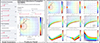 |
Fig. A.1. Preview of the web-based GUI for the HDPmt and plot products. Left panel: View of the main page of the application. Right panel: Example plots that can be produced by the application. |
When the web application starts for the first time, it loads the geometrical model and produces the plots using default parameters. The user can change the parameters of the geometrical model by adjusting the parameter sliders located on the left panel of the application, as shown in Fig. A.1. When the user updates the parameters of the geometrical model, the application re-calculates the model output, and the plots update automatically. From the sliders on the left panel, the user can adjust the disturbance speed and acceleration, as well as the two geometrical parameters, α and ϵ. The application provides three different modes for the user to explore the connection of the disturbance to the field lines and then to calculate the shock parameters at the connection points. In the first mode, the user can select any location, and the application will calculate the connection time and the shock parameters at this point. In the second and third modes, the user selects a longitude, and the application calculates the first connection time, either at the solar surface or at the selected field line.
The user can also select from different visualization options. With the first option, the application visualizes the propagating disturbance in 2D space. These plots are the same as those presented in Fig. 2. The colour of the disturbance lines represents, by default, the propagation time of the disturbance, as shown by the colour bar on the right side. The user can change the colour-coded parameter from the propagation time to the shock parameters, ΘBn or MA. Additionally, in the same plots, the user can select to plot the magnetic field lines instead of the disturbance. Along the field lines, the shock parameters are also depicted. With the next plotting mode, the connection times are visualized as a function of longitude, similar to the plot presented in Fig. 5. We use colour contour lines for ΘBn and black contour lines for MA. With the next plotting mode, the shock geometry and parameters can be visualized as a function of the height or time for every field line. The plot of this mode is similar to those shown in Fig. 7.
At any stage of the analysis, the user can save the plots. Additionally, when the final modelling is ready, the user can download the finalized product in a compressed file. In this file, the parameters of the geometrical model are stored in a JSON (JavaScript Object Notation) file format and the figures in a PNG format. The HDPmt remains under active development and future features will include complex magnetic field configurations for the user to select, more shock parameters to process, and other options.
All Figures
|
Fig. 1. Sketch of the geometrical model of the disturbance. The red circles depict the disturbance front location at different time steps. The blue circle represents the Sun and it is centred at the axis origin. We label the geometrical parameters we used in the model. The labels rsh and Rsh are the distance of a given point, P, located at the disturbance from the solar centre (O) and the disturbance centre (C), and φ is the ∡ COP angle, i.e. the longitudinal separation angle from the disturbance source region. |
| In the text | |
|
Fig. 2. Two views of the propagating disturbance (coloured circles) using the geometrical model at the same expansion speed (Vexp = 800 km s−1), but with two different values for the α parameter. We used α = 0.25 for the top panel and α = 0.75 for the bottom panel. The yellow circle represents the Sun and it is centred at the axis origin. At t = 0 the disturbance is located at the Sun’s surface. |
| In the text | |
|
Fig. 3. Disturbance connection times as a function of the longitudinal separation angle from the eruption site for different model parameters. We use, in the left panels, constant α and varying expansion speed. In the middle panels, we use constant expansion speed and varying α. In the right panels, we use constant speed at the apex and varying ϵ. |
| In the text | |
|
Fig. 4. Sketch of the geometrical model of the disturbance employed in the current study that shows the different points, angles, and vectors that we define in the text and are needed to calculate the ΘBn angle. |
| In the text | |
|
Fig. 5. Disturbance connection times as a function of the longitudinal separation angle from the eruption site for an expansion speed of 800 km s−1 and varying α values among the different panels. The blue curves show the times that the disturbance connects to field lines for the first time, the solid black curves show the time that the disturbance connects at the same field lines at the solar surface. The coloured curves show the connection times when the disturbance has a specific ΘBn at the connected field lines. The dashed black curves show the time when ΘBn = 45° (oblique geometry). For the calculation of ΘBn, we assumed that the field lines are Parker spirals (ΘBr ≠ 0°). The inset plot in each of the panels shows the propagating disturbance (coloured circles) for the different set of parameters used. |
| In the text | |
|
Fig. 6. Plots similar to those presented in Fig. 5, showing the disturbance connection times as a function of the longitudinal separation angle. Here an expansion speed of 800 km s−1 and α = 0.8 are used in both panels. The black contour lines show the evolution of MA values for different angles and times. The MA were calculated using two different coronal models for the variation in density with the heliocentric distance. For the left panel, we used the Saito model and for the right panel, we used the Newkirk model. |
| In the text | |
|
Fig. 7. Evolution of the shock parameters, ΘBn (top panel) and MA (bottom panel), as a function of time. |
| In the text | |
|
Fig. A.1. Preview of the web-based GUI for the HDPmt and plot products. Left panel: View of the main page of the application. Right panel: Example plots that can be produced by the application. |
| In the text | |
Current usage metrics show cumulative count of Article Views (full-text article views including HTML views, PDF and ePub downloads, according to the available data) and Abstracts Views on Vision4Press platform.
Data correspond to usage on the plateform after 2015. The current usage metrics is available 48-96 hours after online publication and is updated daily on week days.
Initial download of the metrics may take a while.