| Issue |
A&A
Volume 668, December 2022
|
|
|---|---|---|
| Article Number | L9 | |
| Number of page(s) | 7 | |
| Section | Letters to the Editor | |
| DOI | https://doi.org/10.1051/0004-6361/202245021 | |
| Published online | 13 December 2022 | |
Letter to the Editor
The mixing of dust and gas in the high latitude translucent cloud MBM 40
1
Dipartimento di Fisica, Università di Pisa, Largo Bruno Pontecorvo 3, Pisa, Italy
e-mail: monaci93@gmail.com; steven.neil.shore@unipi.it
2
Department of Physics and Astronomy, University of Georgia, Athens, GA 30602-2451, Greece
e-mail: loris@uga.edu
Received:
20
September
2022
Accepted:
25
October
2022
Context. High latitude molecular clouds (hereafter HLMCs) permit the study of interstellar gas dynamics and astrochemistry with good accuracy due to their proximity, generally clear lines of sight, and lack of internal star-forming activity which can heavily modify the physical context. MBM 40, one of the nearest HLMCs, has been extensively studied, making it a superb target to infer and study the dust-to-gas mixing ratio (DGMR).
Aims. The mixing of dust and gas in the interstellar medium remains a fundamental issue to keep track of astrochemistry evolution and molecular abundances. Accounting for both molecular and atomic gas is difficult because H2 is not directly observable and H I spectra always show different dynamical profiles blended together which are not directly correlated with the cloud. We used two independent strategies to infer the molecular and atomic gas column densities and compute the dust-to-gas mixing ratio.
Methods. We combined H I 21 cm and 12CO line observations with the IRAS 100 μm image to infer the dust-to-gas mixing ratio within the cloud. The cloud 21 cm profile was extracted using a hybrid Gaussian decomposition where 12CO was used to deduce the total molecular hydrogen column density. Infrared images were used to calculate the dust emission.
Results. The dust-to-gas mixing ratio is nearly uniform within the cloud as outlined by the hairpin structure. The total hydrogen column density and 100 μm emissivity are linearly correlated over a range in N(Htot) of one order of magnitude.
Key words: ISM: clouds / ISM: molecules / dust, extinction
© The Authors 2022
 Open Access article, published by EDP Sciences, under the terms of the Creative Commons Attribution License (https://creativecommons.org/licenses/by/4.0), which permits unrestricted use, distribution, and reproduction in any medium, provided the original work is properly cited.
This article is published in open access under the Subscribe-to-Open model. Subscribe to A&A to support open access publication.
1. Introduction
The admixture of dust and gas is an essential, but poorly determined, property of the interstellar medium. It affects the modeling of radiative balance, moderates astrochemical processes, and affects star formation within molecular clouds (for the theoretical aspect see, e.g., Lee et al. 2017; Tricco et al. 2017; Marchand et al. 2021; for the observational picture, e.g., Reach et al. 2017). The widely adopted value for the mass ratio in our Galaxy is ∼100 − 150 (Hildebrand 1983), but it varies in other galaxies (Young et al. 1986) and even in clouds in our Galaxy (Reach et al. 2015)1.
The usual procedure to obtain the dust-to-gas ratio (hereafter DGR) infers the neutral hydrogen column densities from the dust extinction which is then used to obtain the dust mass. Alternatively, atomic resonance transitions have been used to infer the atomic column densities, but these are altered by density-dependent depletion in the gas phase and from the spotty sampling of any intervening clouds because of the sparse coverage by stars and extragalactic sources. The sparseness of background sources also complicates the distance determination of clouds using standard methods such as star counting, Wolf diagrams, or multiband extinction measurements (e.g., Sun et al. 2021; Lv et al. 2018; Liljestrom & Mattila 1988). These techniques are hampered by the proximity of the translucent and high latitude molecular clouds (see, e.g., Magnani & Shore 2017). Moreover, different lines of sight through these clouds may sample very different structures (e.g., Lombardi et al. 2014) . If the DGRs differ, this complicates extinction corrections and inferences about the cloud masses based on infrared imaging. It is now possible, however, to obtain the atomic column densities directly following the completion of all-sky H I surveys that complement the infrared maps obtained for Galactic and cosmological surveys.
The object of our study, MBM 40, is a small molecular structure embedded in a larger H I flow (Shore et al. 2003). The molecular gas distribution has been discussed extensively (Magnani et al. 1985, MBM; Lee et al. 2002; Shore et al. 2003, SMLM; Shore et al. 2006, SLCM; Chastain et al. 2009, CCM10). The CO(1-0) molecular gas distribution is complex with the denser gas in a hairpin structure surrounded by a diffuse envelope. The distance to the cloud is 93 pc (Zucker et al. 2019) and previous studies (Magnani et al. 1996b; SMLM; CCM10) have derived a molecular mass of 20–40 M⊙. There is no evidence of star formation despite a rigorous search (Magnani et al. 1996a). This cloud provides an exemplar of a non-star-forming medium where no internal processing has affected the dust properties. We should, therefore, see a more nearly pristine presentation of the DGR and its uniformity than would be obtained from a more active source.
2. Data
We have used a range of archival data for this study. We briefly describe here the individual data sets.
2.1. GALFA
The Galactic Arecibo L-Band Feed Array HI (GALFA-HI, Peek et al. 2011,) is an extended survey between −1° ≲δ ≲ 38° with an angular resolution of 4′ and a 0.184 km s−1 spectral resolution using the William E. Gordon 305-m telescope at the Arecibo Observatory (Peek et al. 2018)2. We used the narrow bandwidth data repository (see Peek 2017) centered at 0 km s−1; each spectrum has 2048 channels spanning |vLSR| ≲ 188 km s−1. We used ancillary data furnished with the GALFA datacube to correct for stray radiation and cropped the PPV datacube in position to match the extension and velocity (|vLSR| ≲ 15 km s−1) of MBM 40, which is detected between ∼2 and ∼4 km s−1 in molecular gas. The top panel of Fig. 1 shows an example of a GALFA narrowband spectrum (within the range |vLSR|≤20 km s−1) with a signal-to-noise ratio (S/N) ∼ 60; each spectrum within the cloud has a similar S/N.
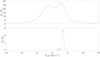 |
Fig. 1. Sample spectra of MBM 40 used in this study. Top panel: single GALFA spectrum at α = 242.7583° ,δ = +21.8084° (J2000.0), in the lower part of the western ridge of MBM 40. Bottom panel: sample FCRAO 12CO spectrum near the same position as the H I, obtained by averaging 64 spectra in an 8 × 8 pattern to enhance the S/N. The vertical dashed line shared by two plots indicates the bulk velocity of the cloud (3.35 km s−1). The H I spectrum shows the brightness temperature (TB), and the 12CO spectrum is in terms of the radiation temperature (TR). |
2.2. FCRAO
The 12CO observations were obtained using the Five College Radio Astronomy Observatory (FCRAO3) in early 2000. The full datacube is composed of 24 576 frequency-switched spectra with a velocity resolution of about 0.05 km s−1. We used only the 56 central channels centered at 3 km s−1. The average rms noise value is 0.7 K (Shore et al. 2003). The 12CO radiation temperature (TR) was calculated taking the antenna temperature and then dividing by ηfssηc, where ηfss is the forward-scattering and spillover efficiency (≃0.7) and ηc is the source filling factor, which we assumed to be unity (see SMLM for a complete discussion of FCRAO observations). The bottom panel of Fig. 1 shows the equivalent FCRAO 12CO profile near the same position of the H I GALFA spectrum. The H I profile shows different components, one of which is compatible with the MBM 40 bulk velocity of ∼3 km s−1.
The H I and 12CO temperature contours for a restricted velocity range are shown in Fig. 2. Here we identify two positions to which we refer in the following sections.
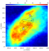 |
Fig. 2. H I brightness temperature at 3.4 km s−1 with integrated line 12CO intensity (black contours at levels 2, 3, and 4 K km s−1). White circles denote the positions to which we refer in the text. In this velocity slice (very near the molecular cloud bulk velocity), the H I emission and 12CO emission (position A) are anticorrelated. |
2.3. IRAS 100 μm dust map
For the dust distribution, we used the IRAS 100 μm IRIS images that have a spatial resolution of about 2′ (Miville-Deschênes & Lagache 2005). These were published after our first study of MBM 40 and have reduced striping, improved zodiacal light subtraction, and a zero level compatible with DIRBE. The image is an interpolated 50 × 50 pixel matrix with the same H I and 12CO spatial resolution centered at  ,
,  . We did not use Planck data for the principal study because the spatial resolution is slightly lower and further reduced by a required interpolation to a common coordinate grid (from galactic to equatorial). We show in the Appendix, however, that our conclusions are unchanged based on Planck.
3. Data analysis
3.1. Velocity slices
The comparison between 12CO and H I profiles in different velocity slices is shown in Fig. 3. Because the spectral resolution of H I is coarser than 12CO, a linear interpolation was performed to match the velocity resolution of the FCRAO data (see the next subsection for further details). The H I is more extended in velocity than the molecular gas traced by 12CO. It appears as a “cocoon” (Shore et al. 2003; Verschuur 1974) around cloud molecular gas and shows some internal structures. We note that H I is present at both lower and higher velocities (i.e., v < 2.25 km s−1 or v > 4 km s−1) where no 12CO is present, tracing foreground and background gas.
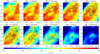 |
Fig. 3. H I velocity slices (color scale) compared to the same 12CO velocity slices (black contours). Contours span from 1 K to 5 K in steps of 1 K. The white circle in the 3 km s−1 panel marks position A in the western ridge. |
The H I spatial resolution is sufficient to compare the atomic and molecular gas structures mapped by 12CO. The velocity slices show an anticorrelation between atomic and molecular gas, especially at position A, marked by a white circle in the 3 km s−1 slice in Fig. 3. The 12CO enhancement is associated with a lower atomic gas column density, indicative of a phase transition. This condensation is visible in all velocity slices.
3.2. Data rebinning and interpolation
The 21 cm and 12CO maps differ in spectral and spatial resolutions. To compare these data, spectral and spatial linear interpolations were performed. Each H I spectrum was linearly interpolated using the 12CO FCRAO velocities (Δv = 0.05 km s−1) as query points. The final spectral H I resolution is 3.5 times higher than the original GALFA resolution. Each H I spectrum has been checked for artifacts and, although linear interpolation is sensitive to S/N, in our case S/N is over 60 for each spectrum. We then performed a 2D linear interpolation for both H I and FCRAO data to a common 50 × 50 pixel grid, covering about  in RA and 1° in Dec. Consequently, using this procedure at each position yields linked GALFA and FCRAO spectra with the same velocity resolution.
3.3. H I profile decomposition
Each H I profile is a blend of multiple components. Because the 21 cm transition is almost always optically thin for lines of sight toward high-latitude clouds, the full line of sight contributes to the observed profile, not only to gas associated with MBM 40, and significant effort was made to decompose each H I spectrum into simpler Gaussian components (see Murray et al. 2021; Lindner et al. 2015; Pingel et al. 2013). In this work we effected a two-step decomposition of each profile guided by velocity information from 12CO as explained below. We used Gaussian profiles to separate the foreground and background as well as cloud neutral hydrogen. The 12CO observations constrain a velocity window in which the cloud is embedded, so it is possible to use this information to trim the H I spectra. We emphasize that the choice of Gaussian fitting was used only to select that gas that is connected to the cloud. This is different from recent Gaussian decomposition studies aimed at characterizing the fine structure of the cold neutral medium (e.g., Murray et al. 2021).
We started the H I decomposition by subtracting a very broad, diffuse component (see, Verschuur & Magnani 1994) from each GALFA profile, fitting a Gaussian only to the wings of the profile outside the interval −7.55 ≤ vLSR ≤ 7.35 km s−1, and then we fit a second Gaussian to the residual emission. Figure 4 (left panel) shows an example of the procedure.
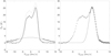 |
Fig. 4. Left panel: subtraction of extremely diffuse gas from H I sample profile. Bold gray lines are wings fitted by a single Gaussian (black dashed line) and the gray dashed line is the section we excluded from the fit; the solid black line is the result of the subtraction, where the diffuse component is severely reduced. Right panel: narrow component extraction: crosses indicate points below 2 km s−1 which we suppose are not directly linked with gas traced by 12CO and which were excluded for the narrow Gaussian fit (black solid line). Circles denote points we used for the fit. |
We excluded positions where there is no clear double profile (i.e., where only diffuse gas is present in the neighborhood of MBM 40), and we fit only the redward wing of each H I residual emission, avoiding points below 2 km s−1 (see Fig. 4, right panel). This procedure cannot map all the gas because we do not know the parent distribution; however, the narrow Gaussian component is at least proportional to the total gas connected with MBM 40.
3.4. Molecular and atomic gas column density
If H I is optically thin, as in MBM 40, and if we assume that one temperature dominates each velocity channel, then the total atomic hydrogen column density is given by the following (see for example Draine 2010):
where TB,H I(v) is the brightness temperature in K and v is the velocity in km s−1.
The molecular hydrogen column density, N(H2), was obtained using the integrated 12CO line in TR multiplied by a conversion factor (XCO in units of cm−2 K−1 km−1 s):

where W(CO) is the velocity-integrated 12CO radiation temperature.
The value of XCO is not constant in the Galaxy or even inside the same cloud (Bolatto et al. 2013), and it is a source of systematic uncertainty. Cotten & Magnani (2013) found that for MBM 40, the XCO factor spans from (0.6 to 3.3) × 1020 with an average of 1.3 × 10²⁰: we adopted this value as well as a systematic uncertainty of about a factor of two. For each FCRAO position, we evaluated N(H2) as follows:
where TR, CO(v) is the radiation temperature for 12CO (cf. SMLM).
Figure 5 shows the derived column densities for atomic and molecular hydrogen. Using Eqs. (1) and (3), we obtain N(Htot) = 2N(H2) + N(H I) within the cloud boundary.
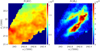 |
Fig. 5. Total column density of H I (left panel) and H2 (right panel). Outside the jagged boarders visible via N(H I), the column densities were not calculated due to a lack of 12CO emission. We note that near position A, there is a deficit in atomic hydrogen where an enhancement in 12CO is present. |
Figure 6 shows N(Htot). The enhancement is quite steep inside the cloud, where the total column density reaches N(Htot)≈16 × 1020 cm−2. We assumed 93 pc as the distance of the cloud (Zucker et al. 2019). Thus, the spatial separation between diffuse gas and the maximum hydrogen column density near position A is ≈0.18 pc, similar to that in 12CO, where the 12CO fades out more or less ten beams away. The cloud shows a broad atomic gas environment within the N(Htot)=2 × 1020 cm−2 contour (i.e., the outermost contour in Fig. 6) where the 12CO is too faint to be detected with reasonable integration times. The distribution of atomic gas is consistent with Shore et al. (2003), where it was modeled with a “cocoon” shape, but using higher fidelity from GALFA revealed some internal structure. Position B (the red dot on the top of Fig. 6) shows 12CO weak lines with virtually no 13CO.
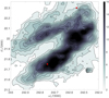 |
Fig. 6. Total hydrogen column density. The colorbar values must be multiplied by a factor of 1020. Red dots indicate the positions discussed in Fig. 2. |
3.5. Dust-to-gas mixing ratio (DGMR)
The DGMR was obtained using the IRIS 100 μm image. We linearly interpolated the image to obtain a 50 × 50 matrix, in which each pixel has a relative H I and 12CO spectra, so we were able to directly perform a simple division to obtain the DGMR. The mean 100 μm of the MBM 40 complex is a few MJy sr−1 and the hydrogen column density is about 1020 cm−2, so we scaled the latter by 10−20 to obtain comparable values with dust emission and then used the following ratio:
where E100 is the total emission of the IRIS 100 μm image and N(Htot) is the total hydrogen column density.
The derived ratio (Fig. 7) is nearly constant within the complex, indicating that the dust and gas are well mixed. We tested the robustness of our procedure by calculating the DGMR using the complete H I spectra, that is without Gaussian decomposition and including the atomic gas over all velocities. The result is nearly the same because the majority of gas is in molecular form (mapped by 12CO). Considering the full H I velocity range, the N(H I) is nearly doubled, but it accounts for about 30% of the total gas. However, without any Gaussian decomposition, the result is much more sensitive to the XCO factor: if we use a lower value, that is to say 0.6 (instead of 1.3), the DGMR changes abruptly and the MBM 40 cloud is barely visible. Conversely, if we decompose the H I profiles, the DGMR remains constant and also the cloud structure is clearly visible. Therefore, we can conclude that not all H I gas mapped by GALFA is linked with MBM 40, but only the narrow component that we extracted. The qualitative appearance from the map in Fig. 7 is quantified by the linearity of the relation of the scatterplot of the total gas column density versus 100 μm emissivity (see Fig. 8).
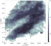 |
Fig. 7. Map of DGMR. The colorbar values are expressed in 1020 MJy sr−1 cm2. Red dots indicate the same positions as reported in Fig. 2. |
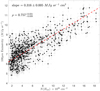 |
Fig. 8. Scatter plot of the total column density versus 100 μm emissivity showing a linear relation. The red dashed line is the best fit with a slope of 0.316 ± 0.005 MJy sr−2 cm2 and a correlation coefficient |
4. Discussion and conclusions
We have shown that the dust is well mixed with gas within the translucent cloud MBM 40, both in densest and rarefied regions, indicating that HLMCs similar to MBM 40 are ideal comparisons for modelling how dust affects gas condensation. Liseau et al. (2015) used a different molecule, N2H+ instead of CO which they argued would be more condensed, to study the dust-to-gas mass ratio in ρ Oph, a dense star-forming region. In contrast, we are only concerned with the degree to which the atomic and molecular gas, and the dust, are mixed within this region. Consequently, we do not need to make any assumptions about the intrinsic dust properties, only that the dust temperature is approximately constant across the cloud. This is valid for MBM 40, as confirmed by the Planck dust temperature map.
Murray et al. (2021) provide a detailed picture of the neutral hydrogen column densities and optical depths of diffuse gas at high Galactic latitudes. Their mean value for N(H I), around 2 × 1020 cm−2, is similar to the highest values we have for the cocoon of MBM 40. In contrast, within the cloud boundaries, the neutral hydrogen is depleted relative to inferred H2 and there we find a total hydrogen column density an order of magnitude greater (Fig. 6), similar to the much coarser result presented in SMLM. The maximum in N(Htot) corresponds to the minimum in N(H I).
As Murray et al. found for their sample, the gas in MBM 40 is not associated with any large structure, such as a supernova remnant or bubble, but it appears to be a transition to molecular gas within a more extended neutral hydrogen filamentary shear flow. The cloud-associated atomic gas is connected in space and radial velocity to more extended regions at distances up to 10 pc in which there is no evidence for excess IRIS 100 μm emission, even in those locations where N(H I) is about the same as for MBM 40.
The comparatively small scale of the molecular structures in MBM 40 provides a testbed for understanding the phase transition of the diffuse gas in isolated environments. The gas and dust are well mixed regardless of the total gas density. This result should inform turbulent mixing simulations and studies of grain chemistry. Our next paper, which is currently in preparation, will present the dynamical and astrochemical tracers.
Based on observations obtained with Planck (http://www.esa.int/Planck), an ESA science mission with instruments and contributions directly funded by ESA Member States, NASA, and Canada.
Acknowledgments
We thank the Arecibo William E. Gordon Observatory staff and GALFA team for HI 21 cm datacube. The 12CO FCRAO data are obtained from SMLM 2003 study. IRIS infrared images are obtained using the SkyView Virtual Observatory and NASA/IPAC Infrared Science Archive. We also thank the referee for valuable suggestions that extended the discussion.
References
- Bolatto, A. D., Wolfire, M., & Leroy, A. K. 2013, ARA&A, 51, 207 [CrossRef] [Google Scholar]
- Chastain, R. J., Cotten, D., & Magnani, L. 2009, AJ, 139, 267 [Google Scholar]
- Cotten, D. L., & Magnani, L. 2013, MNRAS, 436, 1152 [NASA ADS] [CrossRef] [Google Scholar]
- Draine, B. T. 2010, Physics of the Interstellar and Intergalactic Medium (Princeton: Princeton University Press) [CrossRef] [Google Scholar]
- Hildebrand, R. H. 1983, Quart. J. R. Astron. Soc., 24, 267 [NASA ADS] [Google Scholar]
- Lee, Y., Chung, H. S., & Kim, H. 2002, J. Korean Astron. Soc., 35, 97 [NASA ADS] [CrossRef] [Google Scholar]
- Lee, H., Hopkins, P. F., & Squire, J. 2017, MNRAS, 469, 3532 [NASA ADS] [CrossRef] [Google Scholar]
- Liljestrom, T., & Mattila, K. 1988, A&A, 196, 243 [NASA ADS] [Google Scholar]
- Lindner, R. R., Vera-Ciro, C., Murray, C. E., et al. 2015, AJ, 149, 138 [NASA ADS] [CrossRef] [Google Scholar]
- Liseau, R., Larsson, B., Lunttila, T., et al. 2015, A&A, 578, A131 [NASA ADS] [CrossRef] [EDP Sciences] [Google Scholar]
- Lombardi, M., Bouy, H., Alves, J., & Lada, C. J. 2014, A&A, 566, A45 [NASA ADS] [CrossRef] [EDP Sciences] [Google Scholar]
- Lv, Z.-P., Jiang, B.-W., & Li, J. 2018, ChA&A, 42, 213 [NASA ADS] [Google Scholar]
- Magnani, L., & Shore, S. N. 2017, A Dirty Window (New York: Springer) [CrossRef] [Google Scholar]
- Magnani, L., Blitz, L., & Mundy, L. 1985, ApJ, 295, 402 [NASA ADS] [CrossRef] [Google Scholar]
- Magnani, L., Caillault, J.-P., Hearty, T., et al. 1996a, ApJ, 465, 825 [NASA ADS] [CrossRef] [Google Scholar]
- Magnani, L., Hartmann, D., & Speck, B. G. 1996b, ApJS, 106, 447 [NASA ADS] [CrossRef] [Google Scholar]
- Marchand, P., Guillet, V., Lebreuilly, U., & Mac Low, M.-M. 2021, A&A, 649, A50 [NASA ADS] [CrossRef] [EDP Sciences] [Google Scholar]
- Miville-Deschênes, M.-A., & Lagache, G. 2005, ApJS, 157, 302 [Google Scholar]
- Murray, C. E., Stanimirović, S., Heiles, C., et al. 2021, ApJS, 256, 37 [NASA ADS] [CrossRef] [Google Scholar]
- Peek, J. 2017, GALFA-HI DR2 Narrow Data Cubes [Google Scholar]
- Peek, J., Heiles, C., Douglas, K. A., et al. 2011, ApJS, 194, 20 [NASA ADS] [CrossRef] [Google Scholar]
- Peek, J. E. G., Babler, B. L., Zheng, Y., et al. 2018, ApJS, 234, 2 [Google Scholar]
- Pingel, N. M., Stanimirović, S., Peek, J., et al. 2013, ApJ, 779, 36 [NASA ADS] [CrossRef] [Google Scholar]
- Planck Collaboration IV. 2020, A&A, 641, A4 [NASA ADS] [CrossRef] [EDP Sciences] [Google Scholar]
- Reach, W. T., Heiles, C., & Bernard, J.-P. 2015, ApJ, 811, 118 [NASA ADS] [CrossRef] [Google Scholar]
- Reach, W. T., Bernard, J.-P., Jarrett, T. H., & Heiles, C. 2017, ApJ, 851, 119 [NASA ADS] [CrossRef] [Google Scholar]
- Shore, S. N., Magnani, L., LaRosa, T. N., & McCarthy, M. N. 2003, ApJ, 593, 413 [NASA ADS] [CrossRef] [Google Scholar]
- Shore, S. N., LaRosa, T. N., Chastain, R. J., & Magnani, L. 2006, A&A, 457, 197 [NASA ADS] [CrossRef] [EDP Sciences] [Google Scholar]
- Sun, M., Jiang, B., Zhao, H., & Ren, Y. 2021, ApJS, 256, 46 [NASA ADS] [CrossRef] [Google Scholar]
- Tricco, T. S., Price, D. J., & Laibe, G. 2017, MNRAS, 471, L52 [Google Scholar]
- Verschuur, G. L. 1974, ApJS, 27, 65 [NASA ADS] [CrossRef] [Google Scholar]
- Verschuur, G. L., & Magnani, L. 1994, AJ, 107, 287 [NASA ADS] [CrossRef] [Google Scholar]
- Young, J., Schloerb, F., Kenney, J., & Lord, S. 1986, ApJ, 304, 443 [NASA ADS] [CrossRef] [Google Scholar]
- Zucker, C., Speagle, J. S., Schlafly, E. F., et al. 2019, ApJ, 879, 125 [NASA ADS] [CrossRef] [Google Scholar]
Appendix A: Analysis based the Planck dust maps
A.1. Dust-to-gas mass ratio from Planck
The Planck Legacy Archive (PLA) 4 provides high-level maps, including the dust mass column density. We extracted a dust map for MBM 40 in M⊙ pc−2 and converted our total gas column density to 3.4 mass units to obtain the DGMR (Planck Collaboration IV 2020). The result is shown in Fig. A.1.
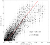 |
Fig. A.1. DGMR using Planck data. |
There is also a DGMR correlation. The greater dispersion results from the reduced resolution caused by coordinate interpolation. But, in addition, the derivation of a single temperature for each pixel affects the correlation isolated to within the cloud. Each pixel was integrated over the line of sight and the spectral energy distribution was modeled for each of these to give a unique temperature, but we also know from the velocity analysis that there is extended foreground and background cold dust that is not associated with MBM 40. We therefore used only the dust emission from the 100 μm IRAS image, without any assumption as to temperature modeling, and we discuss only the mixing ratio.
A.2. Dust temperature using Planck
We selected a PLA region including MBM 40 to check whether the dust temperature is also constant through the whole cloud. The result, shown in Fig. A.2, is that the temperature is nearly constant with a mean value of ∼18 K. It is notable that the internal cloud structure is rendered uniform, confirming that the visible substructures are regions differing in density, not temperature.
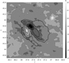 |
Fig. A.2. Dust temperature from Planck data. Black solid contours denote MBM40 (from Planck 545 GHz channel). The two bright sources are galaxies, SDSS J161101.90+215839.6 and SDSS J160808.48+213111.7. |
All Figures
|
Fig. 1. Sample spectra of MBM 40 used in this study. Top panel: single GALFA spectrum at α = 242.7583° ,δ = +21.8084° (J2000.0), in the lower part of the western ridge of MBM 40. Bottom panel: sample FCRAO 12CO spectrum near the same position as the H I, obtained by averaging 64 spectra in an 8 × 8 pattern to enhance the S/N. The vertical dashed line shared by two plots indicates the bulk velocity of the cloud (3.35 km s−1). The H I spectrum shows the brightness temperature (TB), and the 12CO spectrum is in terms of the radiation temperature (TR). |
| In the text | |
|
Fig. 2. H I brightness temperature at 3.4 km s−1 with integrated line 12CO intensity (black contours at levels 2, 3, and 4 K km s−1). White circles denote the positions to which we refer in the text. In this velocity slice (very near the molecular cloud bulk velocity), the H I emission and 12CO emission (position A) are anticorrelated. |
| In the text | |
|
Fig. 3. H I velocity slices (color scale) compared to the same 12CO velocity slices (black contours). Contours span from 1 K to 5 K in steps of 1 K. The white circle in the 3 km s−1 panel marks position A in the western ridge. |
| In the text | |
|
Fig. 4. Left panel: subtraction of extremely diffuse gas from H I sample profile. Bold gray lines are wings fitted by a single Gaussian (black dashed line) and the gray dashed line is the section we excluded from the fit; the solid black line is the result of the subtraction, where the diffuse component is severely reduced. Right panel: narrow component extraction: crosses indicate points below 2 km s−1 which we suppose are not directly linked with gas traced by 12CO and which were excluded for the narrow Gaussian fit (black solid line). Circles denote points we used for the fit. |
| In the text | |
|
Fig. 5. Total column density of H I (left panel) and H2 (right panel). Outside the jagged boarders visible via N(H I), the column densities were not calculated due to a lack of 12CO emission. We note that near position A, there is a deficit in atomic hydrogen where an enhancement in 12CO is present. |
| In the text | |
|
Fig. 6. Total hydrogen column density. The colorbar values must be multiplied by a factor of 1020. Red dots indicate the positions discussed in Fig. 2. |
| In the text | |
|
Fig. 7. Map of DGMR. The colorbar values are expressed in 1020 MJy sr−1 cm2. Red dots indicate the same positions as reported in Fig. 2. |
| In the text | |
|
Fig. 8. Scatter plot of the total column density versus 100 μm emissivity showing a linear relation. The red dashed line is the best fit with a slope of 0.316 ± 0.005 MJy sr−2 cm2 and a correlation coefficient |
| In the text | |
|
Fig. A.1. DGMR using Planck data. |
| In the text | |
|
Fig. A.2. Dust temperature from Planck data. Black solid contours denote MBM40 (from Planck 545 GHz channel). The two bright sources are galaxies, SDSS J161101.90+215839.6 and SDSS J160808.48+213111.7. |
| In the text | |
Current usage metrics show cumulative count of Article Views (full-text article views including HTML views, PDF and ePub downloads, according to the available data) and Abstracts Views on Vision4Press platform.
Data correspond to usage on the plateform after 2015. The current usage metrics is available 48-96 hours after online publication and is updated daily on week days.
Initial download of the metrics may take a while.