| Issue |
A&A
Volume 667, November 2022
|
|
|---|---|---|
| Article Number | A121 | |
| Number of page(s) | 19 | |
| Section | Planets and planetary systems | |
| DOI | https://doi.org/10.1051/0004-6361/202243981 | |
| Published online | 15 November 2022 | |
Chemical evolution in planet-forming regions with growing grains
1
Max Planck Institute for Astronomy (MPIA),
Königstuhl 17,
69117
Heidelberg, Germany
e-mail: eistrup@proton.me
2
Department of Astronomy, University of Virginia,
530 McCormick Road,
Charlottesville, VA
22904, USA
3
School of Physics and Astronomy, University of Exeter,
Stocker Road,
Exeter
EX4 4QL, UK
Received:
9
May
2022
Accepted:
19
July
2022
Context. Planets and their atmospheres are built from gas and solid material in protoplanetary disks. This solid material grows from smaller micron-sized grains to larger sizes in the disks during the process of planet formation. This solid growth may influence the efficiency of chemical reactions that take place on the surfaces of the grains and in turn affect the chemical evolution that the gas and solid material in the disk undergoes, with implications for the chemical composition of the planets.
Aims. Our goal is to model the compositional evolution of volatile ices on grains of different sizes, assuming both time-dependent grain growth and several constant grain sizes. We also examine the dependence on the initial chemical composition.
Methods. The custom Walsh chemical kinetics code was used to model the chemical evolution. This code was upgraded to account for the time-evolving sizes of solids. Chemical evolution was modelled locally at four different radii in a protoplanetary disk midplane (with associated midplane temperatures of 120, 57, 25, and 19.5 K) for up to 10 Myr. The evolution was modelled for five different constant grain sizes, and in one model, the grain size changed with time according to a grain-growth model appropriate for the disk midplane.
Results. Local grain growth, with conservation of the total grain mass, and assuming spherical grains, acts to reduced the total grain-surface area that is available for ice-phase reactions. This reduces the efficiency of these reactions compared to a chemical scenario with a conventional grain-size choice of 0.1 μm. The chemical evolution modelled with grain growth leads to increased abundances of H2O ice. For carbon in the inner disk, grain growth causes CO gas to overtake CO2 ice as the dominant carrier, and in the outer disk, CH4 ice becomes the dominant carrier. Larger grain sizes cause less change the C/O ratio in the gas phase over time than when 0.1 μm sized grains are considered. Overall, a constant grain size adopted from a grain evolution model leads to an almost identical chemical evolution as a chemical evolution with evolving grain sizes. A constant grain size choice, albeit larger than 0.1 μm, may therefore be an appropriate simplification when modelling the impact of grain growth on chemical evolution.
Key words: astrochemistry / planets and satellites: formation / planets and satellites: composition / protoplanetary disks
© C. Eistrup et al. 2022
 Open Access article, published by EDP Sciences, under the terms of the Creative Commons Attribution License (https://creativecommons.org/licenses/by/4.0), which permits unrestricted use, distribution, and reproduction in any medium, provided the original work is properly cited.
This article is published in open access under the Subscribe-to-Open model.
Open Access funding provided by Max Planck Society.
1 Introduction
Planets form in protoplanetary disks around young stars. Exo-planet atmospheres can be observed and chemically characterised, and molecular constituents of the atmospheres can be identified. More generally, carbon-to-oxygen (C/O) ratios of giant exoplanet atmospheres can be retrieved from directly imaged exoplanets with existing facilities. These facilities include the Gravity experiment at ESO’s Very Large Telescope Interferometer (e.g. the exoplanets β Pic b and HR 8799e, see GRAVITY Collaboration 2020; Mollière et al. 2020) and the IGRINS instrument at the Gemini-South Observatory, which was used to retrieve the C/O ratio of the day-side hemisphere of the transiting exoplanet WASP-77Ab (see Line et al. 2021). This chemical characterisation of exoplanet atmospheres will be accelerated by the James Webb Space Telescope (JWST), both in terms of precision (lower uncertainty on C/O ratios) and in terms of the number of exoplanets whose atmospheres will be chemically characterised (~88)1.
Observations of atmospheric compositions of exoplanets are a window into understanding from what the atmospheres and the exoplanets as a whole formed (see e.g. Mordasini et al. 2016). The elemental chemical compositions of exoplanet atmospheres is thought to reflect the combined elemental compositions of the material(s) that went into forming the exoplanet atmospheres. These materials exist in protoplanetary disks and form the planets: gas and solids. The solids have both a refractory (rocky, with high molecular binding energies, and thus high desorption temperatures) and a volatile (icy, with low molecular binding energies and low desorption temperatures) component. The regions of protoplanetary disk midplanes in which volatile species start to freeze out as ices usually have temperatures below 150 K. As the volatile molecule with the highest molecular binding energy (see e.g. Fraser et al. 2001; Penteado et al. 2017), H2O freezes out below this temperature.
Giant exoplanet atmospheres may be formed by run-away accretion of gas surrounding a solid planetary core (as modelled by Madhusudhan et al. 2014; Notsu et al. 2020, with and without protoplanetary disk chemical evolution) and by accretion of ice-covered solids, such as pebbles (see e.g. Lambrechts & Johansen 2012; Bitsch et al. 2019; Trapman et al. 2019). Accretion of pebbles might cause to the material contained in the pebbles to become part of the forming planet and its atmospheres. In other words, the accretion of pebbles by exoplanets could affect the chemical makeup of the planetary atmospheres.
In order to establish a link between the chemical composition of a planetary atmosphere and the formation history of the planet and its atmosphere, it is important to constrain the chemical composition of the volatile ices carried on these pebbles, as they drift inwards from the outer, colder regions of the disk. The volatile ices are of particular importance because these ice components are the main carriers of carbon, oxygen, nitrogen, and sulphur, which go into forming the gas-phase phase species that constitute exoplanet atmospheres. Pebble drift in protoplanetary disks is an active area of research (e.g. Brauer et al. 2008; Birnstiel et al. 2012, 2015), including the accretion of pebbles onto planets (Mordasini et al. 2016; Bitsch et al. 2015, 2020; Bitsch & Johansen 2016; Bitsch & Battistini 2020; Cridland et al. 2016, 2017) and how this accretion affects the resulting compositions of the exoplanet atmospheres (see e.g. Madhusudhan et al. 2014; Drummond et al. 2019).
However, so far, most of these efforts have assumed a predefined set of ice abundances for the pebbles, where this set of abundances remains unchanged from the beginning of the simulations until the pebbles are accreted onto the forming planet. An exception is the desorption of volatile ices, which is assumed to occur when the disk temperature around the pebbles reaches a certain level that corresponds to an icy species that is desorbed into the gas phase.
Booth & Ilee (2019) used a chemical kinetics network through the KROME package (Grassi et al. 2014) to model chemical evolution along with grain growth. They only considered hydrogenation reactions for ices, however, and not two-body ice reactions via the Langmuir-Hinchelwood-mechanism (see e.g. Hasegawa & Herbst 1993; Herbst 2021). Krijt et al. (2020) used a dynamical model setup for grain evolution, including settling from upper disk layers to the midplane, grain growth, and grain drift. They accounted for ice chemistry, but to simplify the treatment of chemical evolution, the chemical network was limited compared to other networks in use (they considered fewer chemical species). From the perspective of chemical modelling, studies such as those by Eistrup et al. (2016, 2018), and Yu et al. (2017) used large chemical networks to model chemical evolution in disk midplanes, but usually assumed constant grains sizes throughout the chemical evolution (typically 0.1 μm) and did not consider material mixing between different regions of the disk.
More recently, Gavino et al. (2021) used the three-phase Nautilus code (Ruaud et al. 2016) and a grain population with multiple grain sizes (constant in time) to model the evolution of volatile ices in a disk. They accounted for the radial and vertical structure of the disk. Furthermore, Van Clepper et al. (2022) modelled chemical evolution during grain growth in the mid-plane and included the effect of turbulent mixing of material from the upper disk layers with the midplane. These two studies are further discussed in Sect. 4.
This paper investigates the chemical evolution in volatile ices on growing grains by comparing grain populations with multiple different constant and evolving grain sizes and using a full chemical kinetics code (two phases). The goal is twofold: We first explore the effects of dust coagulation on ice abundances and then compare chemical evolution during realistic grain growth with chemical evolution, for which we assume simplified grain choices. Based on the results, we can gauge the level of sophistication needed or desired when a treatment of grain growth is included in chemical kinetics codes with the aim to account for grain growth during chemical evolution. This in turn will aid a better understanding of the actual icy compositions of the resulting pebbles, and will provide a better basis for connecting exoplanet atmospheres that are to be characterised with JWST and the evolution of the protoplanetary disk midplane.
2 Methods
The work presented here implements a treatment of grain growth in a comprehensive chemical kinetics code. This approach is novel and necessary for understanding chemical evolution in the more realistic context of growing gains.
The code was modified for this work in order to account for evolving grain sizes, that is, grain growth. While several effects lead to and result from grain growth (e.g. dust settling in the disk midplane, radial drift, and changes in the disk temperature structure and radiation field as opacities change), we focus on one effect of dust growth, namely on the removal of the dust surface area that is available for chemical ice reactions. The surface areas on dust grains are important for the interactions between gasphase species and grain surfaces because of the amount of area that dust grains provide that facilitates the sticking of gas-phase species, as well as the reaction between icy species.
Most chemical kinetics codes for modelling interstellar and protoplanetary disk astrochemistry assume spherical grains with fixed sizes (usually Rgrain = 0.1 μm; see e.g. Fogel et al. 2011; Walsh et al. 2015; Eistrup et al. 2016). However, theoretical work and observational evidence (see e.g. Testi et al. 2014; Birnstiel et al. 2018) both suggest that dust grains grow under conditions found in a disk. It is therefore crucial to develop a better understanding of the effects that grain growth may have on the efficiency of chemical evolution in disk midplanes.
2.1 Dust coagulation
As a starting point for our simulations, we performed local dust coagulation calculations at the disk midplane at four radial locations: 1.5, 5, 20, and 30 AU. The temperatures of gas and grains (assumed to be thermally coupled), gas number densities, and ionisation rates for each considered radius are listed in Table 1.
Assuming that all grains start with a size of 0.1 μm, and maintaining a fixed total solids-to-gas ratio of 0.01, we used a representative particle method to calculate how successive grain-grain collisions alter the local dust size distribution. This method involves calculating collision rates between pairs of representative particles, making use of random numbers to determine which particles will be involved in the next collision event, and when that collision takes place (see e.g. Zsom & Dullemond 2008; Drążkowska et al. 2014; Krijt et al. 2016, for more details). When computing collision rates, we included Brownian motion, differential drift, and turbulence as sources for the relative velocities between pairs of particles (following e.g. Birnstiel et al. 2016), employing an αT prescription for the turbulence, and setting αT = 10−3 when calculating the contribution from turbulent motions using the formulation of Ormel & Cuzzi (2007). We considered perfect sticking and catastrophic fragmentation to be the dominant collision outcomes, with fragmentation occurring above a fixed threshold velocity of υfrag = 10 m s−1, which is often taken to be appropriate for ice-covered grains (Birnstiel et al. 2016). Grain charging was not considered when we determined collision rates or outcomes.
The outcomes of the simulations are evolving sizes for the representative particles that can be combined to produce size distributions or other derived quantities. We capture the evolving size distributions in Fig. 1 by showing the time evolution of two characterising sizes, the mass-dominating grain size Rm (dashed) and surface-area-dominating grain size RA (solid), defined as
 (1)
(1)
where  , and
, and  represent the radius, mass, and surface area of aggregate i (assuming a spherical and compact structure), and ρ = 2.6 g cm−3 is the material density.
At each location, the effects of coagulation and fragmentation are clearly visible. Initially, pairs of small, well-coupled grains collide at low velocities, allowing them to stick and grow, leading to an increasing Rm and RA. The difference between Rm and RA is small during this phase, indicating that the underlying dust size distribution is quite narrow. As the largest grains begin to approach sizes of ≈10−1 cm, however, collision velocities become comparable to the fragmentation velocity, and the ensuing disruptive events lead to the creation of small fragments, the introduction of which quickly decreases RA. Further growth of the largest aggregates stagnates as the fragmentation limit is reached, and Rm begins to level off. After some time, a steady state is reached in which the removal and creation of grains are balanced at every size, and both Rm and RA are constant in time. Typically in protoplanetary disk environments, these fragmentation-limited steady-state distributions are such that most of the mass is contained in large aggregates, while smaller ones dominate the number and surface area (see Birnstiel et al. 2011). The final difference between Rm and RA is about two orders of magnitude, highlighting the broad nature of the final equilibrium situation. Comparing different radial locations in Fig. 1, we see that towards larger disk radii, coagulation timescales become longer, while maximum and equilibrium grain sizes decrease. The behaviour described above agrees with the established picture of (local) dust coagulation (as reviewed e.g. in Birnstiel et al. 2016). We note that our local coagulation calculations do not include radial drift or other forms of material transport between different disk regions; we discuss these limitations further in Sect. 4.6.
In the remaining paper, two grain size cases from Fig. 1 are used for each radius. The first is the case in which the representative grain size RA evolves for each step in the chemical evolution. In this case, RA varies for each time step. This grain size case is therefore denoted “vary”. In the other case, the grain coagulation and fragmentation dynamic has led to a steady-state, or “converged” value for RA, which is the flattening out of the solid profiles for RA in Fig. 1, which occurs for all four radii after the value for RA has peaked. Chemical evolution models assuming this steady-state, or converged, grain size RA, which is derived from grain evolution models, are referred to as “conv” models.
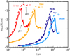 |
Fig. 1 Evolution of the characteristic grain size over time at four heliocentric distances. Curves display the mass-dominating size Rm (dashed) and surface-area-dominating grain size RA (solid). After an initial phase of efficient coagulation (marked by Rm and RA increasing similarly), the creation of fragments in disruptive collisions acts to lower RA and halt growth altogether as a steady state is reached towards the end of the local simulations (shown as open white circles). |
2.2 Volatile chemistry
The chemical kinetics code previously used in Walsh et al. (2015), and Eistrup et al. (2016, 2018) was used. This code includes gas-phase reactions, gas-grain interactions, and grain-surface reactions, including two-body ice reactions and hydrogenation reactions. The chemical kinetics code from Walsh et al. (2015) was modified to enable variations in the grain sizes. This was done by changing the radius Rgrain of dust grains from a global constant in the code to a time variable, where a new value Rgrain is read for every time step.
As shown in Fig. 1, the characteristics (maximum grain size, Rm, and representative grain size, RA) change over time. To simplify the implementation of the dust evolution into the chemical kinetics code, an effective grain size representative of the average grain-surface area per grain RA throughout the whole dust size distribution was derived for each time step. Using RA and changing its value as a function of time allows representing the actual grain surface area of the entire dust grain population by a single grain size for each time step.
The implementation into the code was done as follows: At the first time step, the initial grain size value Rgrain,t=0 was used to calculate chemical reaction rates of effects involving collisions between gas species (atoms, molecules, and electrons) and grains. The size of the grains matters for these effects. In addition to using the initial grain size, the number density of grains per H2 N(grains) is also used. In previous astrochemical models of protoplanetary disk midplanes using fixed-size spherical grains of 0.1 μm (see e.g. Eistrup et al. 2016, 2018), the grain number density was set to N(grains) = 1.3 × 10⁻¹² per H2. This grain size and grain number density correspond to a gas-to-dust mass ratio of 100. In this work, the grain growth is assumed to occur locally (fixed disk midplane radius), that is, without gain or loss of material. In order to conserve the total mass of the dust grains, the grain number density N(grains) evolves from one time step to the next, corresponding to the change in Rgrain, such that the total dust mass is kept constant. This was achieved by scaling N(grains) for all except the first time steps in the following way:
 (2)
(2)
where  is the mass of a single grain of radius R (where ρ(grains) is the mass density of the grains [g cm−3]), and t = n is the nth timestep in the grain size evolution. When the initial grain size differs from 0.1 μm, then the initial grain number density Nt=0(grains) was adjusted from the value 1.3 × 10⁻¹² accordingly to ensure conservation of the dust mass.
The nature of grain growth is that the dust grains collide, coagulate, and grow larger in size. It can accordingly be inferred from Eq. (2) that the grain number density decreases as a function of time. However, for the grain evolution that is considered here, which includes fragmentation of larger dust grain to form smaller grains, smaller grains are replenished, and thereby, a population of small grains is sustained a later stages of grain evolution. Although smaller grains account for a small amount of the total dust mass, they contribute an appreciable amount of surface area to the whole dust population. For this reason, as also shown in Fig. 1, the effective grain size RA actually peaks and subsequently decreases before converging. This evolution of the effective grain size is accounted for by means of the implementation into the chemical kinetics code as outlined in Eq. (2).
The principle behind the treatment of grain sizes in this study is the following: In the actual grain size distribution, it is assumed that all grains are spherical, that they have different sizes, and that for each time step during evolution, there is a certain number of them. In the treatment here, the formal simplification is made that all grains have one size for each time step (solid profiles in Fig. 1). This one size per time step is calculated such that this homogeneously sized population of grains features the same total grain surface area as the original distribution with different sizes, assuming that the cases with homogeneously sized grains and the actual grain distribution with different sizes have identical number densities for the same time step. This principle allows for an implementation of grain growth into the chemical kinetics code where the effective grain size is updated for each time step as a representation of the surface-area-wise behaviour of the actual grain distribution over time.
When the chemical evolution is modelled using various grain sizes at a local radius in a disk midplane without gain or loss of material, it is important to conserve the grain mass density Ngrains per hydrogen atom. That is, as grains grow larger, the number of grains decreases.
For 0.1 μm grains, a gas/dust ratio of 100, and a silicate grain mass-volume density (3 g cm−3), the grain number density per hydrogen atom is Ngrains(0.1 μm) = 1.3 × 10⁻¹². When larger (constant-sized) grains of size Rchoice are assumed, the grain number density is constant, but lower than 1.3 × 10⁻¹², assuming the other factors stay constant. This was accounted for before we ran the chemistry.
This scaling means that for each factor of 10 that the grains are assumed to increase in size (1 μm versus 10 μm), the number density of grains per hydrogen atom decreases by a factor of 1000. When the grains grow for each time step in the chemical evolution, but the grains start out with sizes of Rgrains = 0.1 μm, the adjustment for the grain number density happens automatically in the chemical kinetics code as a consequence of reading in a new grain size.
Dust grains are also important for the balance and exchange of electric charge in disk midplanes. Dust grains can become electrically charged by accreting electrons, and negatively charged grains in turn can neutralise gas-phase cations through collisions. Previous chemical models (Eistrup et al. 2016, 2018) assumed grain number conservation and were initialised with neutral grains alone. However, as these models evolved the chemistry, a fraction of the total grains could become singly negatively charged, and the sum of the number of negatively charged grains and the neutral grains would equate to the initial number of neutral grains.
Like those previous works, this work only assumes neutral and singly negatively charged grains (Gr0 and Gr−, respectively). The chemical models were initialised in a charge-neutral state (in this case, Nt=0(Gr−) = 0, Nt=0(e−) = 0, Nt=0(cations) = 0, and Nt=0(anions) = 0). For a given evolution time step after the t0, featuring a non-zero electron abundance, a fraction of the grains capture electrons and thereby become negatively charged. By using a chemical kinetics code with constant dust mass and dust grain sizes, the sum of the number densities of negatively charged (Nt(Gr−)) and neutral grains (Nt(Gr0)) at time t simply equates to the initial neutral grain number density.
However, when grain growth with dust grain mass conservation is included, as grains are growing the number of grains decreases as the grains grow (see Eq. (2)). When at the beginning of each time step, the number densities of neutral and charged grains are scaled according to Eq. (2), this results is a net change of charge held in grains (net loss, if grains are growing). In order to conserve charge, this change in charge in grains needs to be accounted for elsewhere. There are several possible solutions to this issue: (1) allowing individual grains to carry more than one unit of net charge when they grow, (2) adjusting the efficiency of grain neutralisation reactions from collisions with gas-phase cations, which in turn may affect the cation abundances and charge balance in the gas, and (3) adding/subtracting any gain or loss of grain charge to the electron abundance. The third possibility is the most straightforward to implement, and it may affect the gas-phase cation abundances in a way similar to the second option because an increase/decrease in electron abundances affects the rates of cation-electron recombination reactions.
In the chemical kinetics code, the rates for electron capture by grains and grain-cation recombination are functions of grain radius. The effects on these rates are therefore accounted for when the grain sizes are changed. Moreover, to calculate the grain-cation recombination rates, the chemical kinetic code includes the rate enhancement prescribed by Draine & Sutin (1987).
The second option requires a larger expansion of the chemical kinetics network in order to enable negatively charged grains to add their charges when they stick and grow together, as well as possible electron capture by grains that are already charged. Furthermore, as a destruction pathway for multiply charged grains, full or partial neutralisation of these grains through chargeexchange reactions with cations in the gas phase would need to be added to the chemical network, with one reaction for each cation. This more realistic expansion of the treatment of charged grains in the chemical network will be pursued in future work. In this work, the third option is used to account for charge conservation.
Lastly, two different sets of initial abundances were used in this study: one featuring atomic abundances, and one featuring molecular abundances. The initial abundance sets for these two setups are identical to the abundances used in Eistrup et al. (2016), and we refer to Table 1 in that paper for more insights.
3 Results
In this section we present the results of the chemical modelling. Emphasis is placed on highlighting the differences between chemical abundances for the nominal case with 0.1 μm sized grains and abundances for other grain size choices.
Plots of the absolute abundance evolution (abundance of molecule relative to abundance of hydrogen nuclei (Hnuc) as a function of time for the dominant volatile carriers of elemental C, O, N, and S are shown in Figs. 2–9. Each figure focuses on one combination of a disk midplane radius (1.5, 5, 20, or 30 AU) and an assumption for the initial chemical abundances: MOL represents the initial molecular abundances, and ATOM represents the initial atomic abundances.
The top panel in each figure shows the abundances as a function of evolution time for the dominant volatile carriers of C, O, N, and S and spherical dust grains with a constant size of R = 0.1 μm. The top plots for radii 5 and 30 AU for molecular initial abundances (Figs. 4 and 8) are models that were run with physical conditions and chemical assumptions almost identical to those in the models whose results are shown in panels b and d of Fig. 7 in Eistrup et al. (2018). In the current study, however, three assumptions are different: most importantly, we have updated the molecular binding energy for atomic oxygen from Ebin = 800 to 1660 K, in accordance with the findings of Penteado et al. (2017). Furthermore, we here assumed a static physical disk environment throughout chemical evolution, as opposed to the physically evolving disk that was assumed in Eistrup et al. (2018), and we also now use a different time-step resolution for the chemical modelling.
Our time steps here were adopted from the grain evolution models shown in Fig. 1. Because the grain evolution models capture the grain coagulation and fragmentation effects in short times, which in turn are shorter in the inner than in the outer disk, the time resolution is higher in the inner than in the outer disk. At 1.5 AU, a total of 345 time steps were used to model the chemical evolution from 1 to 107 yr. At 30 AU, 179 time steps were used to model the same timescale. Furthermore, at 1.5 AU, 265 time steps were used to model the chemical evolution from ~300−3 kyr in order to capture the grain growth effects at this location. At 30 AU, 97 time steps were used to model the evolution from ~3−30 kyr, which is the timescale for the grain evolution at this location. The time-step resolutions at 5 and 2 AU fall between these two described cases.
For comparison, Fig. A.1 shows the absolute abundance evolution at the four different midplane radii for a constant grain size of 1mm. This is the largest grain size option in this modelling framework.
The centre and bottom panels of Figs. 2–9 each feature a number of colour-shaded columns, in which each colour represents the evolution of one chemical species. At the bottom of each of these two panels are categorical indicators: the name of the chemical species (matching that in the colour-shaded region itself), and one of six categories:
“vary”, representing chemical models that were run with evolving grain sizes.
“conv”, representing chemical models that were run with a constant grain size, where that size corresponds to the converged value for that radius (see Table 1).
“1em4”, representing chemical models that were run with a constant grain size of R = 10−4 cm = 1 μm.
“1em3”, representing chemical models that were run with a constant grain size of R = 10−3 cm = 10 μm.
“1em2”, representing chemical models that were run with a constant grain size of R = 10−2 cm = 100 μm.
“1em1”, representing chemical models that were run with a constant grain size of R = 10−1 cm = 1 mm.
For each of these grain-size categories, each of the light to dark brown markers in the colour-shaded regions represents the ratio of the abundance of that chemical species at a given evolution time, assuming that choice of grain size and the abundance for the same species at the same evolution time assuming the nominal grain size of 0.1 μm. There are time-step markers for 0.1, 0.5, 1, 2, and 5 Myr (see legend inset) that extend from light to dark brown and also change the marker shape for enhanced clarity (for reference, the five time steps are indicated with vertical dotted lines in the top panels). This choice of displaying the modelling results is intended to clarify which effect grain size choices have on each molecular species, at each radius, and on which timescales. For the centre and bottom panels, the hue of the shading colours is lighter for y-axis ratios above unity and darker for ratios below unity. This is to facilitate evaluating whether a given grain size choice causes the abundance of a certain molecule to be higher or lower than the abundance for the nominal grain size choice.
Lastly, the center panels feature a linear y-scale, whilst the scale is logarithmic in the bottom panels. The reason is that the chemical species in the middle panels are most abundant overall, and therefore undergo relatively smaller changes during evolution than is the case for the species in the bottom panels. The different scales are intended to enhance the dynamical ranges for the panels and facilitate their interpretation. The choice of which species to include in the middle and bottoms panels was made by eye by the main author for all eight figures.
3.1 Chemical comparisons between 0.1 μm grains and other grain size choices
In order to obtain a better impression of the effects that different grain size choices have on the abundance evolution for different chemical species, chemical abundances for different grain size choices relative to abundances for 0.1 μm sized grains are show in Figs. 2–9. The chemical species considered are the dominant volatile carriers of carbon, oxygen, nitrogen, and sulphur, and include H2O, CO2, CH3OH, CO, O2, CH4, C2H6, HCN, NH3, N2, H2S, SO2, SO, and S2. This section describes the key features of these figures.
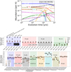 |
Fig. 2 Evolution of chemical abundances, for various choices of grain size. Top panel: evolution of chemical abundances at 1.5 AU starting with molecular (MOL) abundances for a constant grain size of Rgrain = 0.1 μm. Solid profiles show ices (species names starting with G). Dashed profiles show gases. Middle and bottom panels: time- and grain-choice-dependent abundances relative to abundances assuming Rgrain = 0.1 μm. The y-axes are linear for the middle panels and logarithmic for the bottom panels. The vertical dotted lines in the top panel indicate evolution times (0.1, 0.5, 1, 2, and 5 Myr) associated with the markers in the middle and bottom panels. The blue shaded area for H2O ice in the middle panel has additional annotation for guidance: the first vertical category assumes an evolving grain size that grows with time (as annotated above the plot). The second category assumes the final (constant) grain size from the grain growth models, which here, at 1.5 AU, is 34.3 μm (see Table 1). The following four categories represent log-spaced grain size increases (as also indicated with the black arrow, indicating increasing grain sizes extending from categories three through six). This sequence of x-axis categories is identical in all middle and bottom panels in Figs. 2–9. |
3.2 Initial molecular abundances at 1.5 AU and 120 K
The top panel of Fig. 2 features the time evolution for the 12 different volatile species that over a timescale of 10 Myr are the main volatile carriers of C, N, O, and S. The middle panel shows that H2O ice is relatively more abundant with time and for all larger choices of grain sizes than the fiducial size of 0.1 micron. For all larger grain size choices (except for 1 micron), the H2O ice abundance by 5 Myr is more than twice that for the fiducial case. Relating this to the top panel which shows the evolution, this corresponds to a stable H2O abundance after 2 Myr that remains at roughly the initial abundances throughout the evolution.
The abundance of the CO gas in the middle panel for all grain size choices remains the same as for the fiducial size for all time steps. Therefore, it is clear that the elemental oxygen needed for the increased water-ice abundances at larger grain sizes stems from the remaining O-carrying species (CO2 gas, O2 gas, SO gas, and SO2 ice), which are all lower for all grain size choices than the 0.1 micron choice for all evolution times. CH3OH ice does feature some higher relative abundances if the grain sizes vary, converged or 10 microns in size, by 2 Myr of evolution. However, for other sets of grain choices and evolution times, CH3OH ice is also destroyed, contributing elemental О to increase the H2O ice abundance. The top panel also shows that the CO abundance is >10−4 than Hnuc, and given the global C/H ratio of 1.8 × 10⁻⁴ with respect to Hnuc, it therefore follows that CO is the dominant carbon carrier.
Regarding nitrogen carriers, the abundances of N2 (middle panel) is largely unchanged for different grain size choices and different evolution times, and it is the dominant carrier for all parameter choices. For HCN in the lower panel, however, abundance increases of two to four orders of magnitude are seen by longer evolution times (2–5 Myr) for all grain size choices compared with the fiducial size. The source of the elemental nitrogen needed for this increase mainly is NH3 gas, but also destroyed N2. Despite this increase in HCN abundance, it remains a minor carrier of nitrogen, as the baseline HCN abundance for the fiducial grain size after 2–5 Myr evolution is <10−9, placing it outside of the dynamical range of the top panel.
For sulphur, it is clear that for grain sizes that are different from the fiducial size, sulphur is processed more into SO and less into SO2 than in the situation in the top panel. These two carriers feature similar abundances for all choices of grain size and evolution time. H2O becomes an even smaller sulphur carrier than what is shown in the top panel, compared with SO and SO2. The exception for this is a constant grain size choice of 1 micron, for which the abundances of all three carriers are largely similar to that shown in the top panel. This means that only for grain sizes larger than 1 micron do SO2 and SO become the dominant sulphur carriers, and H2S is negligible. That GSO2 and SO dominate the sulphur budget means that they collectively account for ~l–2% of elemental oxygen.
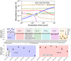 |
Fig. 3 Similar to Fig. 2, but for 1.5 AU, and starting with atomic initial abundances. The converged (conv) grain size at 5 AU is 34.3 μm (see Table 1). We refer to the caption of Fig. 2 for a detailed description. |
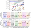 |
Fig. 4 Similar to Fig. 2, but for 5 AU, and starting with molecular initial abundances. The converged (conv) grain size at 5 AU is 12.9 μm (see Table 1). We refer to the caption of Fig. 2 for a detailed description. |
3.3 Initial atomic abundances at 1.5 AU and 120 K
Starting from atomic initial abundances, the effects of grain growth at 1.5 AU are shown in Fig. 3. The abundances of H2O ice (middle panel) increase over time for all grain size choices, except for 1 mm (see the top right panel in Fig. A.1), by up to a factor of 1.7 compared with the fiducial grain size. CO gas, N2 gas, SO2 ice, and SO gas remain at the same abundance levels for all grain size choices and for all time steps, as was the cases for the fiducial grain size. This means that the elemental oxygen contributing to the increase in H2O ice (for all grain sizes except 1 mm) is sourced from oxygen that would otherwise have been carried in CO2 and O2 gas. The abundances of H2S and HCN gas (lower panel) are lower for all grain size choices and time steps than for the fiducial grain size choice, which means (comparing the bottom panel to the top panel) that both species are negligible in abundance for grain choices different from the fiducial size.
3.4 Initial molecular abundances and 5 AU and 57 K
Slightly farther out in the disk midplane, at 5 AU and at a gas and grain temperature of 57 K, the results of grain size choices of chemical evolution starting with a molecular composition are shown in Fig. 4. In the middle planes, it is clear that for all grain size choices other than the fiducial, the H2O ice abundances increase as a function of time. H2O ice becomes up to 2.5 times more abundant by 5 Myr of evolution with grain sizes larger than the fiducial size, which is similar to what was seen for water in Sect. 3.2 (Fig. 2), namely that H2O ice remains at approximately the same abundance throughout evolution. Similarly, like the situation at 1.5 AU, at 5 AU, this increase in abundance of H2O ice is at the expense of the abundances of CO2 ice and O2 gas, with CO2 at 5 AU being in the ice phase, where is was in the gas at 1.5 AU.
CO gas generally is higher in abundance with larger grains sizes, except at 0.1 Myr. For 0.1 and 1mm sized grains, the CO gas abundances from 0.5 Myr and onwards are an order of magnitude higher than for the fiducial grain size at similar time steps.
The CH4 gas abundance is also higher for larger grain sizes compared to the fiducial size for all but the 0.5 Myr time step. For C2H6 ice, only a constant grain size of 1 micron results in higher abundances over all time steps than the fiducial grain size choice.
For nitrogen carriers, most grain size choices, except for 1 mm, lead to higher abundances of NH3 and HCN ices at the expense of N2 gas production. For smaller grain size choices, HCN ices become up to two orders of magnitude more abundant at late time-steps (2–5 Myr) than is the case for the fiducial grain size. When this is compared to the top panel, HCN ice reaches an abundance comparable to that of NH3 and N2 at late time-steps.
For sulphur species, it is noticable that the abundance of H2S gas is lower for most smaller grain size choices than the fiducial grain size. Only for 0.1 and 1mm grain sizes is the H2S abundance higher than in the fiducial case for time steps of 0.5–2 Myr. The abundance of SO2 ices except for the time step at 0.1 Myr is higher for most grain size choices (except 1 micron) at all time steps 0.5 Myr and later than the abundances for the fiducial grain size case.
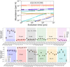 |
Fig. 5 Similar to Fig. 2, but for 5 AU, and starting with atomic initial abundances. The converged (conv) grain size at 5 AU is 12.9 μm (see Table 1). We refer to caption of Fig. 2 for a detailed description. |
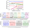 |
Fig. 6 Similar to Fig. 2, but for 20 AU, and starting with molecular initial abundances. The converged (conv) grain size at 20 AU is 7.11 μm (see Table 1). We refer to the caption of Fig. 2 for a detailed description. |
3.5 Initial atomic abundances at 5 AU and 57 K
Starting with atomic abundances at 57 K with the fiducial 0.1 micron-sized grains, the top panel of Fig. 5 shows that CO2 ice and O2 gas quickly (<10 kyr) locks up the majority of С and О and remain the main carriers of С and О throughout the evolution. For larger grain size choices (except for “vary”), much of the О is processed into H2O (~10−4 ice, middle panel) at the expense of the CO2 ice throughout the evolution (bottom panel), while O2 gas remains at ±50% of the level in the top panel throughout the evolution and for all choices of grain sizes. The С that is available for the decreasing abundance of CO2 ice for larger grain sizes is primarily processed into CO gas (bottom panel). Ultimately, these changes mean that O2 gas, CO gas, and H2O ice all have similar abundances when larger grain sizes are assumed.
For N, choices of larger grain sizes generally mean a decrease in HCN ice abundance and an increase in NH3 ice and N2 gas abundances (except for 1mm grains, for which there is no increase in NH3 ice). For S, most of the S carried in SO2 ice in the top panel is processed into H2S gas for choices of larger grain sizes.
3.6 Initial molecular abundances at 20 AU and 25 K
At 25 K, CO and N2 are the only carriers of C, O, and N that are mainly in the gas phase. The top panel in Fig. 6 shows that H2O ice (at ~3 × 10⁻⁴ with respect to H, thereby accounting for ~60% of the elemental O) and CO2 ice (at ~10−4 with respect to H) are the dominant carriers of С and О throughout the chemical evolution. For grain size choices different from the fiducial, the middle panel shows that H2O ice increases slightly (~20%) and CO2 ice decreases slightly, but they both remain the dominant carriers of С and О at all grain size choices and timescales. The CO gas abundance, on the other hand, varies dramatically at different evolution timescales in the bottom panel, but the abundance changes for CO gas as a function of evolution time are similar for different grain size choices. In other words, for larger grain sizes, the choice of grain size does not matter as much for its abundance as the evolution time. The С that is left over from the decreasing CO gas and CO2 abundances is processed into species such as CH4 ice and HCN ice for the largest grain sizes of 0.1−1 mm. This processing into HCN ice in turn leads to a decrease in the abundances of NH3 ice and N2 gas at late evolutionary times, as shown in the middle panel.
At most evolutionary times and for grain sizes of 10 micron (“1em3”) or smaller, some of the С from the decreasing CO2 ice abundance adds to the C2H6 ice abundances. The CH3OH ice abundance decreases more with longer evolution time. It is up to two orders of magnitude lower by 10 Myr of chemical evolution for all grain size choices than it is for the fiducial grain size. Sulphur is processed from SO ice into H2S ice for larger grain size choices. This causes the difference in the abundances of the two species in the top panel to be evened out so that they each carry roughly similar amounts of elemental S by evolutionary times longer than 1 Myr.
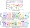 |
Fig. 7 Similar to Fig. 2, but for 20 AU, and starting with atomic initial abundances. The converged (conv) grain size at 20 AU is 7.11 μm (see Table 1). We refer to the caption of Fig. 2 for a detailed description. |
3.7 Initial atomic abundances at 20 AU and 25 K
Figure 7 shows the evolution for a start with atomic abundances at 25 K. Like the situation in Sect. 3.6, H2O ice and CO2 ice are the dominant carriers of С and О throughout the evolution for the fiducial grain size, as shown in the top panel. Interestingly, for the larger grain size choices in the middle and bottom panels, the abundance of H2O ice decreases more and more with longer evolution time, whereas CO2 ice experiences an abundance increase for all larger grain size choices, with the abundance growing larger with evolution time. After 0.5 Myr of chemical evolution, the abundances of these two ices are roughly equivalent (both at ~2 × 10⁻⁴ with respect to H) and stay so until 5 Myr of evolution. For the scenarios with varying grain sizes (vary) and constant grain size at 1 micron (1em4), CO2 is more abundant (by 50–100%) than H2O ice from 0.5 Myr of evolution and onwards.
While the О providing the increase in the CO2 ice abundance comes mainly from a smaller production of H2O ice for larger grain size choices than the fiducial, the middle and bottom panels show that the С carried in the CO2 ice for the larger grain size choices is a result of a lower production of CO gas, CH4 ice, CH3OH ice, C2H6 ice, and HCN ice. That is to say, for larger grain size choices than the fiducial, H2O ice and CO2 ice become the by far dominant carriers of С and O. They account for about 99% of both elements.
For varying grain sizes in the middle panel, N is processed more into NH3 ice and HCN ice with a lower production of N2 gas than in the fiducial case. For all other larger grain size choices, HCN ice is lower in abundance than the two other species, and especially N2 gas increases in abundance, but NH3 ice increases less strongly. For grain size choices larger than 10 microns (1em3), N2 gas is the most abundance N-carrying species until ~2 Myr of evolution, after which point NH3 ice is the most abundant.
For sulphur, larger grain size choices lead to more elemental S being carried in H2S ice than in the fiducial grain size choice. SO2 ice and SO ice are both lower in abundance for larger grain size choices at all evolutionary times than they were for the fiducial choice. However, for the two largest grain size choices, SO ice remains the dominant S-carrier for evolution times 2 Myr.
The top panel shows a ratio of O2-to-H2O ice of 1% for evolutionary times shorter than 0.5 Myr. Furthermore, the bottom panel indicates that for all larger grain size choices, the O2 ice abundance is similar to the abundance for the fiducial grain choice after 1 Myr, and by 0.5 Myr, it is an order of magnitude larger than the abundance for the fiducial grain size choice when grains of 0.1 or 1mm are assumed (1em2 and 1em1, respectively). For the same evolutionary times and grain choices, the middle panel shows that the H2O ice abundance is 25–40% lower than for the fiducial grain size choice. This reflects the underlying abundance condition: from the start of the chemical evolution and up until between 0.1–0.5 Myr of evolution, the abundance ratio O2/H2O ~ 1−25% for grain choices of 0.1 or 1 mm.
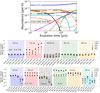 |
Fig. 8 Similar to Fig. 2, but for 30 AU, and starting with molecular initial abundances. The converged (conv) grain size at 30 AU is 3.85 μm (see Table 1). We refer to the caption of Fig. 2 for a detailed description. |
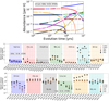 |
Fig. 9 Similar to Fig. 2, but for 30 AU, and starting with atomic initial abundances. The converged (conv) grain size at 30 AU is 3.85 μm (see Table 1). We refer to the caption of Fig. 2 for a detailed description. |
3.8 Initial molecular abundances at 30 AU and 19.5 K
At 19.5 K, all considered species are in the ice phase. For the fiducial grain size in the top panel of Fig. 8, H2O ice is the dominant carrier of O by far throughout the evolution (growing in abundance from ~3−5 × 10⁻⁴). For other grain size choices, the H2O ice abundance is slightly lower there (~20−30%) than for the fiducial grain size at later evolutionary times, but it still accounts for more than 60% of elemental O. CO ice increases in abundance if the grain growth assumption is either the varying, the converged, or the 1 micron grain size relative to the fiducial gain size. For grain sizes larger than these, CO ice is less abundant throughout the chemical evolution than is the case for the fiducial grain size case, with the exception of early evolutionary times (<0.1 Myr), at which point the CO ice abundance is the same as it was in the fiducial grain size case.
C-carrying species such as HCN ice and CH3OH ice generally reach lower abundances for larger grain size choices, whereas the abundances of CH4 ice and CO2 reach higher abundances for larger grain size choices. C2H6 ice reaches higher abundances at early evolutionary times (up to 0.5 Myr) than in the fiducial case, but is lower in abundance for all larger grain size choices for evolutionary times of 1 Myr and longer than in the fiducial case.
For N-carrying species, larger grain size choices lead to higher abundances of N2 ice with longer chemical evolution (see bottom panel), whereas NH3 ice and HCN ice are slightly less abundant for larger grain sizes than for the fiducial grain size choice (see middle panel). However, NH3 ice is the most abundant N-carrying species at all evolutionary times and for all larger grain size choices, although after 1 Myr of evolution, all three molecules feature abundances within a factor of four of each other, and all are >10−6 with respect to H. For sulphur, larger grain size choices lead to lower SO ice abundances and higher H2S abundances relative to the fiducial grain size choice for all evolution times. For grain size choices of 10 microns (1em3) or larger, H2S ice remains the dominant carrier throughout the chemical evolution. However, for grain size choices of either the varying, the converged, or the 1 micron grain size relative to the fiducial gain size, SO ice becomes the dominant S-carrier after ~1 Myr of evolution.
3.9 Initial atomic abundances at 30 AU and 19.5 K
Like the situation starting with molecular abundances at 19.5 K, an assumption of atomic initial abundances also leads to less H2O ice and more CO2 ice produced for longer evolution times and larger grain size choices than is the case for the fiducial grain size choice. Furthermore, since H2O ice and CO2 ice in the top panel of Fig. 9 show similar abundances for evolution times shorter than 0.5 Myr, this means that for larger grain size choices, CO2 ice is the more abundant of the two species until evolution times of ~1 Myr.
The production of CO2 ice for larger grain size choices means than CH3OH ice, CO ice, CH4 ice, and C2H6 ice are much less abundant for the choices than they were for the fiducial choice. The exception to this is CH4 ice. For varying grain sizes as well as for the 1 micron grain size (1em4), it is more abundant than for the fiducial grain size choice. O2 ice varies strongly in abundance depending upon grain size choice and evolution times. However, for evolution times of 0.1 and 0.5 Myr (in the top panel, this is the evolution times with significant O2 ice abundances), the O2 ice abundance is similar to the abundance for the fiducial grain size.
For N-carrying species, HCN ice is much less abundant for larger grain sizes than for the fiducial grain choice, whereas both NH3 ice and N2 ice are more abundance for grain size choices of 10 microns (1em3) or below. For larger grain size choices than this, only N2 ice is more abundant throughout the evolution compared to the fiducial grain size. For S-carrying species, H2O ice generally grows in abundance (for longer evolution times) at the expense of SO ice.
4 Discussion
In this section, the overall trends seen in the model results are highlighted. We also discuss how and under which conditions the modelling of chemistry alongside with grain growth can be simplified for the purpose of easy adoption into astro-chemical modelling frameworks. A key question to answer when implementing grain growth into a chemical kinetics modelling framework as done here is how the changing grain sizes affect which molecules are the dominant carriers of the chemical elements.
4.1 Initial molecular abundances
For 1.5 and 5 AU radii, the H2O ice abundances, which decreased by >2 Myr of evolution time in the (top) plots of Figs. 2 and 4, are seen to decrease only insignificantly at the late evolution times for larger grain size choices (as seen by the net increases in H2O ice abundance for all evolution times and all larger grain size choices in the middle and bottom panels of the two figures). At 20 and 30AU, the H2O ice abundance remains largely at its initial abundance for all larger grain size choices. This means that for all modelling setups starting with initial molecular abundances, the H2O ice abundance largely remains at its initial level and is therefore the dominant molecule and the dominant carrier of elemental oxygen for all choices of grain size. For the largest grain size choice of 1mm, this is shown in the left column in Fig. A.1.
Elemental carbon, on the other hand, becomes distributed across several different species for larger grain size choices. At 1.5 AU, CO gas is the dominant carrier for all grain sizes, including the 0.1 μm. At 5 AU, on the other hand, CO2 ice is the primary carrier, and C2H6 ice is the secondary carrier after 1 Myr of evolution for a grain size of 1 μm (1em4), but when constant grain sizes of 100 μm or 1mm are assumed, CO gas takes over as primary carrier of carbon, and CO2 ice becomes the secondary carrier. At 20 AU, CO2 ice remains the primary carrier (by >0.5 Myr of evolution) for grain sizes of 1 μm−1 mm, but the secondary carbon carrier for 1 mm is C2H6 ice, whereas CH4 ice is the secondary carbon carrier for constant grain sizes of 100 μm−1 mm.
At 30 AU, the top panel of Fig. 8 shows that CO2 ice is the main carbon carrier until ~4 Myr of chemical evolution, at which point C2H6 ice becomes the dominant carrier, with CH4 ice as the secondary carrier. For larger grain sizes of 100 μm−1 mm, CO2 ice is the dominant carrier until evolution times longer than 1 Myr, after which point CH4 ice becomes the dominant carrier, with CO2 ice as secondary carrier.
In summary, while different grain size choices change the absolute abundance of all species, H2O ice remains the main oxygen carrier. For carbon, however, larger grain size choices tend to change the main carbon carrier in the inner disk (1.5−5 AU) from CO2 ice to CO gas and from CO2 ice to CH4 ice in the outer, colder disk (20−30 AU).
4.2 Initial atomic abundances
In the outer, colder disk midplane, at 20 and 30 AU, a comparison between Figs. 7 and 9 and A.1 shows that H2O ice and CO2 ice are the dominant carriers of carbon and oxygen, both when constant 0.1 μm grains and whenany larger grain size choices are assumed. However, while H2O ice is the more abundant of the two for 0.1 μm grains, the CO2 ice abundance increases to become the dominant carrier of elemental carbon and oxygen for larger grain sizes.
For the warmest conditions, at 1.5 AU, CO and O2 gas are the dominant carriers of elemental carbon and oxygen for all choices of grain size. At 5 AU, assuming 0.1 μm size grains, CO2 ice and O2 gas are the dominant carriers, but for larger grain size choices, H2O ice, CO2 ice, O2 gas, and CO gas are all significant carriers of both elements, as shown in the bottom right panel in Fig. A.1, where all these molecules feature abundances within a factor of two of each other for evolution times < 1 Myr. The temperature of 57 K at 5 AU, when purely atomic starting compositions are assumed, therefore might be a sweet spot for developing ice compositions of solid bodies that are not dominated by one or even two species.
Variations in modelled abundances for when the converged grain size is assumed constant (conv) versus assuming the grain size to change for each chemical evolution time step (vary) for the dominant carriers of C and O at the four radii.
4.3 Chemical evolution with evolving grain sizes versus constant grain sizes
This paper has explored and tested a range of different options for implementing grain growth in chemical kinetics in the context of a protoplanetary disk midplane. One important aspect to evaluate about the results is the extent to which accounting for an evolving grain population with a time-dependent grain size distribution has significant impact on the chemical evolution, as compared with a constant grain population (in particular, a constant total grain surface area), inspired by models of grain growth. In other words, the question is whether a realistic chemical evolution can be modelled based on a constant grain size (e.g. the converged grain size RA from the approach taken here) that is adopted from grain growth models, or if it is necessary to evolve grain sizes (RA) for each time step taken in a chemical kinetics model.
Before we address this question, we note that the grain size evolution at 1.5 and 5 AU reaches the converged value for RA by 2.72 and 16.5 kyr of the evolution, respectively (see Table 1). This is on a shorter timescale than 0.1 Myr, which is the first evolution to for which the abundances of molecules are shown in the middle and bottom comparison panels in Figs. 2–9. That is to say, the difference in chemical evolution between the setups with grain growth (vary) and the setup with a constant converged grain size (conv) for radii 1.5 and 5 AU are only different from each other in the first several thousand years of chemical evolution, whereas from ~20 kyr−0.1 Myr of evolution, the two cases are identical. This explains why the evolution of all considered species (for molecular initial abundances) is very similar across the vary and conv cases for 1.5 and 5 AU.
At 20 and 30 AU, the converged grain size is only reached by 0.13 and 0.39 Myr, respectively, which means that by 0.1 Myr of evolution, the chemistry between the vary and conv cases have evolved with different grain sizes RA throughout. By 0.5 Myr of chemical evolution at these two radii, the resulting abundances are more alike across the two grain size cases, and by 1 Myr and longer, the abundances are largely similar.
Table 2 quantifies how much the abundances of the three dominant carriers of carbon and oxygen in the conv grain size case vary relative to their abundances in the vary grain size cases. This table shows that for all radii and all evolution times, the variation between assuming evolving grain sizes and assuming a constant, converged grain size is <1%. This means that, when we assume that the timescale for grain growth to reach a converged representative grain size RA is shorter than twice the first chemical timescale considered (convergence of RA at 30 AU is reached by ~200 kyr; see the solid profiles in Fig. 1; and the first chemical timescale is 100 kyr), then an assumption of the converged grain size throughout evolution will lead to the same chemical abundances of the main carriers of carbon and oxygen, as will grain sizes that evolve with time. For the purpose of modelling chemical evolution in protoplanetary disk midplane settings, it may therefore be an advantageous simplification to run chemical kinetics assuming the RA (t = final) of the grain population at the end of grain growth as a constant grain size, rather than accounting for each change in RA(t) that actually takes place for each chemical time step.
For the larger constant grain sizes considered here other other than vary and conv, different evolution of abundances of all species is seen. We hope that these results and insights can serve as input for future research of chemical evolution, where larger grain sizes are considered.
4.4 Effects of grain growth on C/O ratios in the gas phase
An important factor when planet formation in disks is linked to observed exoplanets is the elemental ratios that are measured in disks and in exoplanet atmospheres. The C/O ratio has long been considered key to forging this link (see e.g. Öberg et al. 2011; Madhusudhan et al. 2014; Eistrup et al. 2016, 2018; Ali-Dib 2017; Mollière et al. 2022), and recently, similar ratios involving N and S have been suggested to overcome the degenaracies resulting from the use of the C/O ratio; see Turrini et al. (2021). It is therefore interesting to consider how the different grain size choices in this work affect the C/O ratio.
Figure 10 shows the C/O ratios for gas-phase species. Different coloured markers indicate the evolution time. The seven types of grain sizes for which chemical models were run are indicated along the x-axis. The left panel shows the situation at 1.5 AU, and the right panel shows it at 5 AU. 20 and 30 AU are not relevant for gas-phase C/O ratios because almost all carbon- and oxygen-carrying species are frozen out at those temperatures (except for CO at 20 AU). The third row in each panel shows the C/O ratio evolution for the fiducial grain size of 0.1 μm. The evolution at both 1.5 and 5 AU for this grain size is comparable to the C/O ratio evolution plot inside and outside, respectively, of the CO2 iceline in Fig. 9a in Eistrup et al. (2018). This is because the same chemical network and the same grain size were used, and only the physical structures vary slightly in these two studies.
At both 1.5 and 5 AU, the C/O ratio evolution in the gas for the fiducial grain size is clearly distinctly different than for the other grain size choices. At 1.5 AU, the grain size choices vary, conv, 1em3, 1em2, and 1em1 all feature similar C/O ratio values with similar time dependences. In all these case, the C/O ratio at 0.1 Myr of evolution is similar to the cases for 1em5 and 1em4, but for longer evolution times, the C/O ratio value in the gas for the five larger grain size choices increases in time, from C/O ~ 0.75 at 0.1 Myr up to C/O ~ 0.95 by 5 Myr of evolution. This upward trend is different from the C/O ratio for the fiducial choice, where the time evolution trend goes from C/O ~ 0.75 at 0.1 Myr to C/O ~ 0.5 at 5 Myr. This means that the gas at 1.5 AU becomes more carbon rich relative to oxygen for larger grain size choices. Because the total amounts of elemental C and O are constants and the two elements can only exist as gas and as ice, this also means that the ice becomes more carbon poor relative to oxygen. This is opposite to the trend shown in Fig. 9a of Eistrup et al. (2018).
At 5 AU, the trend in C/O ratio value is similar (decreasing) for all grain size choices. However, for all other choices than the fiducial choice, the C/O ratio only decreases from C/O ~ 1.2 to C/O ~ 0.9−1.0. For the fiducial case, the final value is much lower, at C/O ~ 0.1. Interestingly, at 5 AU, little change to the C/O ratio values is seen over time after 0.5 Myr of evolution for choices other than the fiducial choice.
Two effects influence these differences in the C/O ratio evolution for the fiducial grain size choice and all other choices: First, for the fiducial grain size, elemental oxygen is processed from H2O ice into O2 gas, which, due to the different molecular binding energies of these two species, serves to move elemental oxygen from the ice to the gas at midplane temperatures between 30−120 K. Figures 2 and 4 show that the decrease in H2O ice abundance and the increase in O2 gas abundance that is shown in the top plots is no longer observ for larger grain size choices. Second, for larger grain size choices, the effect of the ice-phase reaction pathway
 (3)
(3)
is reduced, whereby the CO gas abundance is generally higher and the CO2 ice abundance generally lower for larger grain size choices than for the fiducial choice. Along with the higher abundance of CH4 gas (at 5 AU), all in all, this maintains a large amount of elemental carbon (relative to oxygen) in the gas phase, which keeps the C/O ratios in the gas relatively higher than in the case for the fiducial grain size choice. The reduced efficiency of the chemical reaction pathways described here can be attributed to the fact that for larger grain size choices, the grain surface area for ice chemistry is smaller overall, and thus the effect that grain surface-reactions and gas-grain interactions had for the fiducial case is reduced for larger grain size choices.
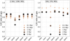 |
Fig. 10 Carbon-to-oxygen ratios for gas-phase species as a function of evolution time steps (colours and markers) for each of the seven grain choices (the third x-axis category, 1em5, is the fiducial grain size of 0.1 μm). Left panel: situation at 1.5 AU, and the right panel at 5 AU. The y-axis scales are identical in both panels. The models for 20 and 30 AU are not plotted because at 20 AU, only CO gas remains in the gas phase, and at 30 AU, all carbon and oxygen carriers are in the ice. |
4.5 Comparison with previous work
While modelling of chemical evolution in disks and modelling of grain growth in disks considered separately are active areas of research, the efforts attempting to combine the two have been limited. When this has been attempted, the research goals werere not always aligned, and it can accordingly be difficult to compare the results. Vasyunin et al. (2011), as well as some references therein, modelled chemical kinetics in a 2D protoplanetary disk, assuming two different constant grain population (and, hence, two different constant RA) as well as a more realistic approach with grain evolution (grain sedimentation from upper disk layers to midplane, as well as grain growth). This work focused more on the effects of grain growth on resulting column densities of various species by modelling chemical evolution in the upper layers of the disk, and not specifically consider the midplane. The results from this study therefore do not directly compare to ours.
Gavino et al. (2021) used 12 different models for grains with varied grains sizes, grain temperatures, UV radiation level, and the considered mechanisms for the formation of H2 on grain surfaces. Out of their 12 models, 6 assumed a constant grain size of 0.1 μm, 4 took into account a full population of grains of different sizes where different sizes could be assigned different temperatures, and 2 used a single grain size representative of the grain-surface area in the full grain population for three different radii. The latter two models, with a representative grain size RA, followed the same concept as the conv models in the current work. Whereas Gavino et al. (2021) explored the effects of a full grain distribution with varying temperatures on the chemical evolution without grain evolution, the current work explored the effects of a single grain size with a single temperature (per time step) with the single grain size evolving in time (but the temperature remained constant).
It was predicted by Gavino et al. (2021) that when grain sizes larger than 0.1 μm are included, carbon is processed into CO2 ice for warmer conditions, and into CH4 ice for colder conditions. This approximately agrees with the trends seen in the current work, where larger grains lead to a change in the main carbon carrier from CO2 ice to CH4 ice. Gavino et al. (2021) also argued that a grain size distribution allowing for different temperatures for the different size populations allows a production of COMs in the warmer grains that is not seen when a representative grain size RA is assumed with a constant temperature. Eistrup et al. (2018), amongst others, also reported that grains with temperatures in the ranges of 30−40 K produced more COMs than colder grains. However, it might be argued that assuming a representative grain size RA for each radius in the midplane (as was done in the current work), with more radial bins than here, and with dust temperatures changing from bin to bin could result in similar effects because bins with grain temperatures of 23−40 K would be encountered. This could facilitate the production of COMs, without assuming a grain size and temperature distribution at each radius.
4.6 Impact of dust dynamics
While relative velocities between aggregates were included in the dust coagulation routine described in Sect. 2.1, the models presented here are static in the sense that there is no material exchange from one region to another. As increasingly large aggregates (i.e. pebbles) are formed, however, their increased aerodynamical Stokes number causes them to partially decouple from the gas. They virtually settled in the disk midplane and migrate radially inwards in the case of a smooth gas disk (e.g. Birnstiel et al. 2016; Misener et al. 2019). As most of the solid mass is contained in the larger aggregates, these processes can displace large numbesr of species that are present as ices, leading to a complex and time-dependent redistribution of those species in particular whose snowlines are crossed by drifting or settling pebbles (e.g. Cuzzi & Zahnle 2004; Krijt et al. 2018; Booth & Ilee 2019).
Recently, a treatment of vertical settling of dust grains from the upper layers of the disk towards the disk midplane was implemented into a chemical kinetics model by Van Clepper et al. (2022). They modelled chemical evolution of ices on grains and pebbles in a midplane, accounting for the effect of turbulent mixing with the upper layers of the disk. Their grain growth model for the midplane included the continual inflow of grains that settled from the upper layers of the disk, as well as radial diffusion in the midplane. Neither of these effects are considered in this paper. However, they only considered one growth model with grains larger that 0.1 μm, whereas this paper considered one dynamic (vary), and several different larger constant grain sizes. Van Clepper et al. (2022) found CO gas to be depleted from the surface layers of a disk by one to two orders of magnitude, assuming a turbulence of α = 10−3. This was achieved by a combination of ice sequestration and decreasing UV opacity, both driven by pebble growth, as they concluded. The radii they considered (30 and 40 AU) featured associated midplane temperatures of ~24 and ~21 K, respectively (see their Fig. 2), which were similar to the temperatures considered here at 20 and 30 AU.
Krijt et al. (2020) used a compact set of chemical species (including H2O, CO, CO2, CH4, and CH3OH) as primary carriers of elemental carbon and oxygen, with a network of ionisation, dissociation, and hydrogenation reactions to exchange carbon and oxygen between the above five main carriers. This network being smaller, it enabled an easier implementation of chemical evolution into a grain evolution model, which included both sedimentation of grains to the midplane, growth, and radial drift of the solids. They argued that all grain evolution effects they included were necessary in order to reproduce the observed low abundances of CO gas in protoplanetary disks (e.g. Zhang et al. 2017, 2019, 2020). For the chemical evolution scenarios presented here, the CO gas abundance is generally similar or higher if larger grain sizes than the fiducial size are assumed (at 1.5, 5 and 20 AU) and shorter evolution times are considered (<2 Myr), highlighting the potential of dynamical effects to alter the resulting behaviour.
All these modelling efforts indicate that the fields of astro-chemistry and grain evolution in protoplanetary disks are aiding each other constructively. This merging of the fields to improve the understanding of planet formation is important and necessary: in the coming years, ALMA will continue to expand our understanding of the chemical (gas) condition for planet formation in protoplanetary disks, and the JWST will soon start exploring the compositions of protoplanetary disk ices and the make-up of exoplanet atmospheres through numerous observation programs. The wealth of new data from these facilities is poised to test the modelling frameworks and predictions that are now published or are underway, and to provide a great leap for the understanding of how planets and their atmospheres form.
5 Caveats for our model assumptions
5.1 Treatment of charge conservation with grain growth
In this work, the conservation of charge with grain growth was chosen to be accounted for by varying the electron abundance for each chemical and grain growth time step. Other options, as mentioned in Sect. 2, would be to adjust the abundances of either cations or anions, or to allow for multiply charged grains. In the case of multiply charged grains, it would be interesting to investigate how an approach like the one prescribed in Fujii et al. (2011) could improve the treatment. This is left for future investigations.
5.2 Fractal grain growth and fluffy aggregates: Is spherical grain growth realistic?
Realistic grain growth is not a process of growing from one sphere to another, but rather of micron-sized (or smaller) grains colliding and sticking (see e.g. Windmark et al. 2012). It is also suggested from theory that grain growth can lead to formation of fluffy aggregates (Kataoka et al. 2015). These are highly fractal structures that despite resulting from collisions and sticking between its constituent micron-sized grains have not compacted into a spherical shape. Fluffy aggregates thus feature effective grain surface areas comparable to the sum of the original grain surface areas of its constituents. In this case, grains growing as fluffy aggregates do not reduce their grain surface area available for surface reaction as compared to the case with 0.1 μm sized grains.
Realistic grain growth, however, is likely in between compact, spherical growth and growth as fluffy aggregates (until these compact). If grains in a protoplanetary disk midplane are assumed to have a representative size (spherical or not) or, for instance, RA = 10 μm, then it is likely that the 10 μm case in this current work underestimates the available grain surface area available for ice reactions. However, the current work provides chemical evolution results for 1 μm grains as well, and so it is possible that the actual chemical evolution scenario can be assessed by assuming abundances in between the results for 1 μm and 10 μm.
6 Conclusion
Protoplanetary disks facilitate both grain growth and chemical reactions leading to chemical evolution. However, until recently, models of grain growth did not account for chemical reactions, and models of chemical evolution did not account for grain growth. This paper set out to improve this treatment by implementing a treatment of grain growth into the WALSH chemical kinetics code. Results from modelling of grain growth were used to model chemical evolution as grain sizes varying with time and assuming a representative grain size throughout the chemical evolution. Discrete, constant grain sizes of 0.1 μm, 1 μm, 10 μm, 100 μm, and 1 mm were also assumed, and their effects on the chemical evolution were assessed. We list some key finding below.
Local, spherical grain growth, without gain or loss of material over time, acts to reduce the total area on the surfaces of grains that is available for ice reaction of the grain surfaces. This reduces the efficiency of chemical reactions in the ice, while gas-phase reactions proceed unaffected. This also means that ice chemistry produces fewer new molecules that could desorb into the gas phase and partake in the gas-phase chemistry.
Starting from a set of molecular initial abundances, all choices for grain growth lead to sustained or increased abundances of H2O ice, which is the main carrier of elemental oxygen. In the inner, warmer disk midplane, larger grain sizes cause CO gas to become the dominant carrier of elemental carbon instead of CO2 ice. For lower temperatures in the outer, colder disk midplane, choices of larger grain sizes cause CH4 ice to become the dominant carbon carrier.
The magnitude of change in the C/O ratio in the gas phase is smaller when grain growth or large grains are considered than when 0.1 μm sized grains are considered.
Generally, assuming that the grain growth timescale is similar to or shorter than the chemical timescale, choosing a more realistic grain growth setup with grain sizes varying with time produces almost identical resulting abundances as does a more simplified setup, where a constant grain size is used throughout the chemical evolution (a size with an associated total grain surface area that mimics the area in the actual evolved grain distribution). A simplified grain size setup in chemical kinetics codes with one constant (but realistic) grain size may therefore be favoured.
When modelling the chemical evolution that takes place in ices on growing grains in protoplanetary disk midplanes, it may be a reasonable approximation to assume a constant grain size throughout chemical evolution, instead of accounting for changing grain sizes for each modelling time step of chemical evolution. The choice of constant grain size should, however, be larger than the fiducial size of 0.1 μm, in order to reflect the grown dust grain population in the disk midplane.
Acknowledgements
The authors thank the referee, Tommaso Grassi, for suggesting valuable comments and improvements. C.E. thanks the Virginia Initiative for Cosmic Origins Postdoctoral Fellowship Program at the University of Virginia for support. Research for this paper was supported by the European Research Council under the Horizon 2020 Framework Program via the ERC Advanced Grant Origins 83 24 28.
Appendix A Chemical Abundances as a Function of Time for a Constant Grain size Rgrain = 1mm
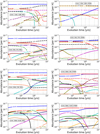 |
Fig. A.1 Evolution of chemical abundances at all radii (top to bottom: 1.5, 5, 20, and 30 AU) for a constant grain size of Rgrain = 1mm. Solid profiles show ices (species names starting with G). Dashed profiles show gases. Left panels: Chemical models initiated with all elemental C, O, N, and S in molecules (MOL in inset). Right panels: Chemical models initiated with all elemental C, O, N, and S as atoms (ATOM in inset). Vertical dotted lines indicate the evolution times used for the analysis: 0.1Myr, 0.5Myr, 1Myr, 2Myr, and 5Myr. |
References
- Ali-Dib, M. 2017, MNRAS, 467, 2845 [NASA ADS] [CrossRef] [Google Scholar]
- Birnstiel, T., Ormel, C. W., & Dullemond, C. P. 2011, A&A, 525, A11 [NASA ADS] [CrossRef] [EDP Sciences] [Google Scholar]
- Birnstiel, T., Klahr, H., & Ercolano, B. 2012, A&A, 539, A148 [NASA ADS] [CrossRef] [EDP Sciences] [Google Scholar]
- Birnstiel, T., Andrews, S. M., Pinilla, P., & Kama, M. 2015, ApJ, 813, L14 [NASA ADS] [CrossRef] [Google Scholar]
- Birnstiel, T., Fang, M., & Johansen, A. 2016, Space Sci. Rev., 205, 41 [Google Scholar]
- Birnstiel, T., Dullemond, C. P., Zhu, Z., et al. 2018, ApJ, 869, L45 [CrossRef] [Google Scholar]
- Bitsch, B., & Battistini, C. 2020, A&A, 633, A10 [NASA ADS] [CrossRef] [EDP Sciences] [Google Scholar]
- Bitsch, B., & Johansen, A. 2016, A&A, 590, A101 [NASA ADS] [CrossRef] [EDP Sciences] [Google Scholar]
- Bitsch, B., Lambrechts, M., & Johansen, A. 2015, A&A, 582, A112 [NASA ADS] [CrossRef] [EDP Sciences] [Google Scholar]
- Bitsch, B., Izidoro, A., Johansen, A., et al. 2019, A&A, 623, A88 [NASA ADS] [CrossRef] [EDP Sciences] [Google Scholar]
- Bitsch, B., Trifonov, T., & Izidoro, A. 2020, A&A, 643, A66 [EDP Sciences] [Google Scholar]
- Booth, R. A., & Ilee, J. D. 2019, MNRAS, 487, 3998 [CrossRef] [Google Scholar]
- Brauer, F., Dullemond, C. P., & Henning, T. 2008, A&A, 480, 859 [NASA ADS] [CrossRef] [EDP Sciences] [Google Scholar]
- Cridland, A. J., Pudritz, R. E., & Alessi, M. 2016, MNRAS, 461, 3274 [Google Scholar]
- Cridland, A. J., Pudritz, R. E., Birnstiel, T., Cleeves, L. I., & Bergin, E. A. 2017, MNRAS, 469, 3910 [NASA ADS] [CrossRef] [Google Scholar]
- Cuzzi, J. N., & Zahnle, K. J. 2004, ApJ, 614, 490 [NASA ADS] [CrossRef] [Google Scholar]
- Draine, B. T., & Sutin, B. 1987, ApJ, 320, 803 [NASA ADS] [CrossRef] [Google Scholar]
- Drążkowska, J., Windmark, F., & Dullemond, C. P. 2014, A&A, 567, A38 [NASA ADS] [CrossRef] [EDP Sciences] [Google Scholar]
- Drummond, B., Carter, A. L., Hébrard, E., et al. 2019, MNRAS, 486, 1123 [NASA ADS] [CrossRef] [Google Scholar]
- Eistrup, C., Walsh, C., & van Dishoeck, E. F. 2016, A&A, 595, A83 [NASA ADS] [CrossRef] [EDP Sciences] [Google Scholar]
- Eistrup, C., Walsh, C., & van Dishoeck, E. F. 2018, A&A, 613, A14 [NASA ADS] [CrossRef] [EDP Sciences] [Google Scholar]
- Fogel, J. K. J., Bethell, T. J., Bergin, E. A., Calvet, N., & Semenov, D. 2011, ApJ, 726, 29 [NASA ADS] [CrossRef] [Google Scholar]
- Fraser, H. J., Collings, M. P., McCoustra, M. R. S., & Williams, D. A. 2001, MNRAS, 327, 1165 [Google Scholar]
- Fujii, Y. I., Okuzumi, S., & Inutsuka, S.-I. 2011, ApJ, 743, 53 [Google Scholar]
- Gavino, S., Dutrey, A., Wakelam, V., et al. 2021, A&A, 654, A65 [NASA ADS] [CrossRef] [EDP Sciences] [Google Scholar]
- Grassi, T., Bovino, S., Schleicher, D. R. G., et al. 2014, MNRAS, 439, 2386 [Google Scholar]
- GRAVITY Collaboration (Nowak, M., et al.) 2020, A&A, 633, A110 [NASA ADS] [CrossRef] [EDP Sciences] [Google Scholar]
- Hasegawa, T. I., & Herbst, E. 1993, MNRAS, 261, 83 [NASA ADS] [CrossRef] [Google Scholar]
- Herbst, E. 2021, Front. Astron. Space Sci., 8, 207 [NASA ADS] [CrossRef] [Google Scholar]
- Kataoka, A., Muto, T., Momose, M., et al. 2015, ApJ, 809, 78 [Google Scholar]
- Krijt, S., Ciesla, F. J., & Bergin, E. A. 2016, ApJ, 833, 285 [Google Scholar]
- Krijt, S., Schwarz, K. R., Bergin, E. A., & Ciesla, F. J. 2018, ApJ, 864, 78 [Google Scholar]
- Krijt, S., Bosman, A. D., Zhang, K., et al. 2020, ApJ, 899, 134 [NASA ADS] [CrossRef] [Google Scholar]
- Lambrechts, M., & Johansen, A. 2012, A&A, 544, A32 [NASA ADS] [CrossRef] [EDP Sciences] [Google Scholar]
- Line, M. R., Brogi, M., Bean, J. L., et al. 2021, Nature, 598, 580 [NASA ADS] [CrossRef] [Google Scholar]
- Madhusudhan, N., Amin, M. A., & Kennedy, G. M. 2014, ApJ, 794, L12 [Google Scholar]
- Misener, W., Krijt, S., & Ciesla, F. J. 2019, ApJ, 885, 118 [NASA ADS] [CrossRef] [Google Scholar]
- Mollière, P., Stolker, T., Lacour, S., et al. 2020, A&A, 640, A131 [Google Scholar]
- Mollière, P., Molyarova, T., Bitsch, B., et al. 2022, ApJ, 934, 74 [CrossRef] [Google Scholar]
- Mordasini, C., van Boekel, R., Mollière, P., Henning, T., & Benneke, B. 2016, ApJ, 832, 41 [Google Scholar]
- Notsu, S., Eistrup, C., Walsh, C., & Nomura, H. 2020, MNRAS, 499, 2229 [Google Scholar]
- Öberg, K. I., Murray-Clay, R., & Bergin, E. A. 2011, ApJ, 743, L16 [Google Scholar]
- Ormel, C. W., & Cuzzi, J. N. 2007, A&A, 466, 413 [NASA ADS] [CrossRef] [EDP Sciences] [Google Scholar]
- Penteado, E. M., Walsh, C., & Cuppen, H. M. 2017, ApJ, 844, 71 [Google Scholar]
- Ruaud, M., Wakelam, V., & Hersant, F. 2016, MNRAS, 459, 3756 [Google Scholar]
- Testi, L., Birnstiel, T., Ricci, L., et al. 2014, Protostars and Planets VI (Tucson: University of Arizona Press), 339 [Google Scholar]
- Trapman, L., Facchini, S., Hogerheijde, M. R., van Dishoeck, E. F., & Bruderer, S. 2019, A&A, 629, A79 [NASA ADS] [CrossRef] [EDP Sciences] [Google Scholar]
- Turrini, D., Schisano, E., Fonte, S., et al. 2021, ApJ, 909, 40 [Google Scholar]
- Van Clepper, E., Bergner, J. B., Bosman, A. D., Bergin, E., & Ciesla, F. J. 2022, ApJ, 927, 206 [NASA ADS] [CrossRef] [Google Scholar]
- Vasyunin, A. I., Wiebe, D. S., Birnstiel, T., et al. 2011, ApJ, 727, 76 [NASA ADS] [CrossRef] [Google Scholar]
- Walsh, C., Nomura, H., & van Dishoeck, E. 2015, A&A, 582, A88 [NASA ADS] [CrossRef] [EDP Sciences] [Google Scholar]
- Windmark, F., Birnstiel, T., Ormel, C. W., & Dullemond, C. P. 2012, ApJ, 544, L16 [Google Scholar]
- Yu, M., Evans, N. J., II, Dodson-Robinson, S. E., Willacy, K., & Turner, N. J. 2017, ApJ, 841, 39 [NASA ADS] [CrossRef] [Google Scholar]
- Zhang, K., Bergin, E. A., Blake, G. A., Cleeves, L. I., & Schwarz, K. R. 2017, Nat. Astron., 1, 0130 [NASA ADS] [CrossRef] [Google Scholar]
- Zhang, K., Bergin, E. A., Schwarz, K., Krijt, S., & Ciesla, F. 2019, ApJ, 883, 98 [Google Scholar]
- Zhang, K., Schwarz, K. R., & Bergin, E. A. 2020, ApJ, 891, L17 [Google Scholar]
- Zsom, A., & Dullemond, C. P. 2008, A&A, 489, 931 [NASA ADS] [CrossRef] [EDP Sciences] [Google Scholar]
All Tables
Variations in modelled abundances for when the converged grain size is assumed constant (conv) versus assuming the grain size to change for each chemical evolution time step (vary) for the dominant carriers of C and O at the four radii.
All Figures
|
Fig. 1 Evolution of the characteristic grain size over time at four heliocentric distances. Curves display the mass-dominating size Rm (dashed) and surface-area-dominating grain size RA (solid). After an initial phase of efficient coagulation (marked by Rm and RA increasing similarly), the creation of fragments in disruptive collisions acts to lower RA and halt growth altogether as a steady state is reached towards the end of the local simulations (shown as open white circles). |
| In the text | |
|
Fig. 2 Evolution of chemical abundances, for various choices of grain size. Top panel: evolution of chemical abundances at 1.5 AU starting with molecular (MOL) abundances for a constant grain size of Rgrain = 0.1 μm. Solid profiles show ices (species names starting with G). Dashed profiles show gases. Middle and bottom panels: time- and grain-choice-dependent abundances relative to abundances assuming Rgrain = 0.1 μm. The y-axes are linear for the middle panels and logarithmic for the bottom panels. The vertical dotted lines in the top panel indicate evolution times (0.1, 0.5, 1, 2, and 5 Myr) associated with the markers in the middle and bottom panels. The blue shaded area for H2O ice in the middle panel has additional annotation for guidance: the first vertical category assumes an evolving grain size that grows with time (as annotated above the plot). The second category assumes the final (constant) grain size from the grain growth models, which here, at 1.5 AU, is 34.3 μm (see Table 1). The following four categories represent log-spaced grain size increases (as also indicated with the black arrow, indicating increasing grain sizes extending from categories three through six). This sequence of x-axis categories is identical in all middle and bottom panels in Figs. 2–9. |
| In the text | |
|
Fig. 3 Similar to Fig. 2, but for 1.5 AU, and starting with atomic initial abundances. The converged (conv) grain size at 5 AU is 34.3 μm (see Table 1). We refer to the caption of Fig. 2 for a detailed description. |
| In the text | |
|
Fig. 4 Similar to Fig. 2, but for 5 AU, and starting with molecular initial abundances. The converged (conv) grain size at 5 AU is 12.9 μm (see Table 1). We refer to the caption of Fig. 2 for a detailed description. |
| In the text | |
|
Fig. 5 Similar to Fig. 2, but for 5 AU, and starting with atomic initial abundances. The converged (conv) grain size at 5 AU is 12.9 μm (see Table 1). We refer to caption of Fig. 2 for a detailed description. |
| In the text | |
|
Fig. 6 Similar to Fig. 2, but for 20 AU, and starting with molecular initial abundances. The converged (conv) grain size at 20 AU is 7.11 μm (see Table 1). We refer to the caption of Fig. 2 for a detailed description. |
| In the text | |
|
Fig. 7 Similar to Fig. 2, but for 20 AU, and starting with atomic initial abundances. The converged (conv) grain size at 20 AU is 7.11 μm (see Table 1). We refer to the caption of Fig. 2 for a detailed description. |
| In the text | |
|
Fig. 8 Similar to Fig. 2, but for 30 AU, and starting with molecular initial abundances. The converged (conv) grain size at 30 AU is 3.85 μm (see Table 1). We refer to the caption of Fig. 2 for a detailed description. |
| In the text | |
|
Fig. 9 Similar to Fig. 2, but for 30 AU, and starting with atomic initial abundances. The converged (conv) grain size at 30 AU is 3.85 μm (see Table 1). We refer to the caption of Fig. 2 for a detailed description. |
| In the text | |
|
Fig. 10 Carbon-to-oxygen ratios for gas-phase species as a function of evolution time steps (colours and markers) for each of the seven grain choices (the third x-axis category, 1em5, is the fiducial grain size of 0.1 μm). Left panel: situation at 1.5 AU, and the right panel at 5 AU. The y-axis scales are identical in both panels. The models for 20 and 30 AU are not plotted because at 20 AU, only CO gas remains in the gas phase, and at 30 AU, all carbon and oxygen carriers are in the ice. |
| In the text | |
|
Fig. A.1 Evolution of chemical abundances at all radii (top to bottom: 1.5, 5, 20, and 30 AU) for a constant grain size of Rgrain = 1mm. Solid profiles show ices (species names starting with G). Dashed profiles show gases. Left panels: Chemical models initiated with all elemental C, O, N, and S in molecules (MOL in inset). Right panels: Chemical models initiated with all elemental C, O, N, and S as atoms (ATOM in inset). Vertical dotted lines indicate the evolution times used for the analysis: 0.1Myr, 0.5Myr, 1Myr, 2Myr, and 5Myr. |
| In the text | |
Current usage metrics show cumulative count of Article Views (full-text article views including HTML views, PDF and ePub downloads, according to the available data) and Abstracts Views on Vision4Press platform.
Data correspond to usage on the plateform after 2015. The current usage metrics is available 48-96 hours after online publication and is updated daily on week days.
Initial download of the metrics may take a while.