| Issue |
A&A
Volume 666, October 2022
|
|
|---|---|---|
| Article Number | A97 | |
| Number of page(s) | 10 | |
| Section | Cosmology (including clusters of galaxies) | |
| DOI | https://doi.org/10.1051/0004-6361/202244404 | |
| Published online | 13 October 2022 | |
A pair of early- and late-forming galaxy cluster samples: A novel way of studying halo assembly bias assisted by a constrained simulation⋆
1
Institute of Astronomy and Astrophysics, Academia Sinica (ASIAA), Taipei 10617, Taiwan
e-mail: This email address is being protected from spambots. You need JavaScript enabled to view it.
2
Kobayashi-Maskawa Institute for the Origin of Particles and the Universe (KMI), Nagoya University, Nagoya 464-8602, Japan
3
Kavli Institute for the Physics and Mathematics of the Universe, The University of Tokyo Institutes for Advanced Study, The University of Tokyo, Chiba 277-8583, Japan
4
Shanghai Astronomical Observatory, Shanghai 200030, PR China
5
Department of Physics, Massachusetts Institute of Technology, Cambridge, MA 02139, USA
6
Graduate Institute of Astrophysics and Department of Physics, National Taiwan University, Taipei 10617, Taiwan
7
Department of Physics, National Chung Hsing University, Taichung 402, Taiwan
8
Institute for Advanced Research, Nagoya University, Nagoya 464-8601, Japan
Received:
3
July
2022
Accepted:
1
August
2022
Abstract
The halo assembly bias, a phenomenon referring to dependencies of the large-scale bias of a dark matter halo other than its mass, is a fundamental property of the standard cosmological model. First discovered in 2005 from the Millennium Run simulation, it has been proven very difficult to be detected observationally, with only a few convincing claims of detection so far. The main obstacle lies in finding an accurate proxy of the halo formation time. In this study, by utilizing a constrained simulation that can faithfully reproduce the observed structures larger than 2 Mpc in the local universe, for a sample of 634 massive clusters at z ≤ 0.12, we found their counterpart halos in the simulation and used the mass growth history of the matched halos to estimate the formation time of the observed clusters. This allowed us to construct a pair of early- and late-forming clusters, with a similar mass as measured via weak gravitational lensing, and large-scale biases differing at the ≈3σ level, suggestive of the signature of assembly bias, which is further corroborated by the properties of cluster galaxies, including the brightest cluster galaxy and the spatial distribution and number of member galaxies. Our study paves a way to further detect assembly bias based on cluster samples constructed purely on observed quantities.
Key words: large-scale structure of Universe / cosmology: observations / galaxies: clusters: general
Full Tables 1 and 2 are only available at the CDS via anonymous ftp to cdsarc.u-strasbg.fr (130.79.128.5) or via http://cdsarc.u-strasbg.fr/viz-bin/cat/J/A+A/666/A97
© Y.-T. Lin et al. 2022
 Open Access article, published by EDP Sciences, under the terms of the Creative Commons Attribution License (https://creativecommons.org/licenses/by/4.0), which permits unrestricted use, distribution, and reproduction in any medium, provided the original work is properly cited.
This article is published in open access under the Subscribe-to-Open model. This email address is being protected from spambots. You need JavaScript enabled to view it. to support open access publication.
1. Introduction
It has been well known for more than a decade that, although the large-scale bias of dark matter halos is primarily a function of halo mass, it also has secondary dependencies on other halo properties such as the formation time, concentration, and spin (e.g., Gao et al. 2005; Jing et al. 2007). Such dependencies are loosely referred to as assembly bias (AB; see e.g., Mao et al. 2018; Wechsler & Tinker 2018). As AB is a subtle, yet solid feature of the cold dark matter model with a cosmological constant (ΛCDM; e.g., Contreras et al. 2021), a solid observational detection of the phenomenon will serve as a critical validation of the model.
In this study, we restrict ourselves to investigating the AB as manifested by the differences in the halo formation time; that is, we aim to detect differences in the large-scale bias for halos of the same mass, but with different formation times. Numerous studies have shown that the amplitude of halo AB is dependent on the halo mass (and to some degree, the definition of halo formation time and even the definition of a halo itself; see Mansfield & Kravtsov 2020 for details). In general, it is more prominent for low-mass halos, while less so at the massive end such as galaxy clusters. In our earlier attempt to detect AB in halos of a mass comparable to that of the Milky Way (∼1012 M⊙), we did not find convincing evidence for AB (Lin et al. 2016). It is likely because our proxy for the halo formation time, namely the mean stellar age of central galaxies derived from spectra provided by the Sloan Digital Sky Survey (SDSS; York et al. 2000), is not of sufficient accuracy.
Using a large sample of SDSS redMaPPer clusters (Rykoff et al. 2014), Miyatake et al. (2016, hereafter M16) claimed a strong detection of AB, which unfortunately turned out to be mainly due to the projection effect; in brief, the formation time proxy used by M16, namely the spatial concentration of photometrically selected potential cluster member galaxies, is contaminated by large-scale correlated structures along the line of sight, which mimics the AB signal (More et al. 2016; Zu et al. 2017; Sunayama & More 2019). It is thus clear that, in the pursuit of detection of the AB signal, one of the main challenges is to have a robust proxy for the halo formation time (while ensuring similar halo masses between early- and late-forming samples is another challenging aspect).
Here we present a novel approach for the estimation of the halo formation time, which makes heavy use of the forward-modeling-based numerical simulation Elucid (Wang et al. 2016). Elucid is designed to reproduce the structures larger than ∼2 Mpc observed by the SDSS main galaxy sample (Strauss et al. 2002) out to a redshift z = 0.12. As such, by matching a galaxy cluster sample drawn from the cluster and group catalog of Yang et al. (2007, hereafter Y07), we can find a one-to-one correspondence between the observed clusters and the simulated halos, whereby the cluster formation time is derived from the halo mass growth history. This method then allows us to split the cluster sample into early- and late-forming subsamples; based on mass measurements from weak gravitational lensing (WL) and the large-scale bias derived from cluster-galaxy cross correlation, we show that, within the ΛCDM framework, a pair of early- and late-forming cluster samples exhibits the signature of AB at the ≳3σ level, which will facilitate the study of halo AB at the high-mass end (see also Zu et al. 2021).
This paper is structured as follows: in Sect. 2 we describe the key elements of our analysis. We construct a pair of early- and late-forming cluster samples that exhibits the AB signal, and examine the properties of cluster galaxy population of the samples in Sect. 3. We discuss the validity of our approach in Sect. 4, and implications and prospects of the method developed in this paper in Sect. 5. Throughout this paper we adopt a WMAP5 (Komatsu et al. 2009) ΛCDM model, where Ωm = 0.258, ΩΛ = 0.742, H0 = 100 h km s−1 Mpc−1 with h = 0.71, σ8 = 0.8, which is employed by Elucid (Wang et al. 2014, 2016). All optical magnitudes are in the AB photometry system (Oke & Gunn 1983, which should not to be confused with assembly bias).
2. Methodology
Here we provide an overview of the main elements of our analysis. The basis of this work, the constrained simulation Elucid, is presented in Sect. 2.1. Our cluster sample, and the way we matched it to the simulated halos from Elucid, are described in Sect. 2.2. We then turn to our key observables, clustering and WL measurements, in Sects. 2.3 and 2.4. We describe our method for measuring the cluster galaxy surface density profiles in Sect. 2.5.
2.1. Constrained simulation Elucid
The goal of producing the Elucid simulation is to reproduce the large-scale structures as observed by SDSS, which would then allow us to “visualize” the distribution of dark matter, and better understanding how galaxies populate dark matter halos. The methodology behind Elucid can be found in Wang et al. (2014). Basically, a nonlinear density field is provided to a Hamiltonian Markov chain Monte Carlo (HMC) algorithm combined with particle-mesh (PM) dynamics, which is able to reconstruct the initial linear density field. That density field is then evolved to the present-day with high resolution N-body simulations.
For the specific simulation used in this work, the nonlinear density field was constructed based on the group catalog of Y07, which itself was based on SDSS data release 7 (DR7; Abazajian et al. 2009). Given that the galactic systems in the Y07 catalog are complete down to a mass limit of ≈1012 h−1 M⊙ at z ∼ 0.12, the nonlinear density field was estimated using only halos above that mass limit and in the redshift range 0.01 − 0.12, lying within the northern Galactic cap region of the DR7 footprint. The reconstructed initial density field was then evolved with 30723 particles in a 500 h−1 Mpc box, using a modified version of GADGET-2 (Springel et al. 2005; Wang et al. 2016). Tests based on detailed mock galaxy samples showed that the typical scatter between the true (nonlinear) density field and the reconstructed one is 0.23 dex when smoothed over a scale of 2 h−1 Mpc (Wang et al. 2016), which is about the typical size of a massive cluster, and is thus a good match for our purpose.
2.2. Galaxy cluster sample selection
To match real clusters to the simulated halos in Elucid, we used the model C version of the Y07 catalog. As shown in Wang et al. (2016), only part of the SDSS DR7 footprint is covered in the reconstructed volume, and we ended up with 644 clusters with mass M200m ≥ 1014 h−1 M⊙. Here the mass is defined within a radius r200m, within which the mean density is 200 times the mean density of the universe at the redshift of the cluster. We note that the mass estimates of galactic systems in Y07 is based on a method similar in spirit to subhalo abundance matching (e.g., Conroy et al. 2006; Wechsler & Tinker 2018), that is, given the dark matter halo mass function, one assumes the total stellar mass (or luminosity) content of a galactic system is directly proportion to the halo mass, and thus one can “assign” a halo mass to observed groups and clusters to halos of the same spatial density.
The matching between the Y07 clusters and the Elucid halos was done in the following fashion: for a given cluster with mass M1, we searched all simulated halos with a distance to the position of the cluster in the simulation less than 4 h−1 Mpc, which is the length scale adopted in Wang et al. (2016) for the density field reconstruction. We have properly taken into account the redshift space distortion effect of clusters, by moving dark matter halos to redshift space using their peculiar velocities along the line of sight. Let us denote the mass of halos that lie within the sphere as M2. For all halos with mass satisfying |log(M1/M2)| < 0.5, we selected the one with the smallest |log(M1/M2)| as the matched halo. As demonstrated by Wang et al. (2016), such criteria of matching enable > 95% of clusters more massive than 1014 h−1 M⊙ to be associated with a halo in Elucid. If no halo satisfied the above condition, then the cluster was discarded from the sample. Out of 644 clusters, we found 634 matches this way1.
For the clusters with a counterpart halo, we extracted the mass growth history of the main subhalo (that is, simply following the main trunk of the merger tree), and derived several formation time indicators, such as z80, z50, z20, and zmah. While the first three correspond to the redshifts when a halo first reaches 80%, 50% and 20% of its final (z = 0) mass, the last quantity was obtained by first fitting the mass growth history by the form
 (1)
(1)
with the Levenberg–Marquardt algorithm for minimization of the least squares, and then setting zmah ≡ 2/α − 1 (Wechsler et al. 2006).
Finally, we note that the cluster center defined by the Y07 cluster finding algorithm is a luminosity weighted position based on the distribution of member galaxies, and the brightest cluster galaxy (BCG) is not necessarily located at the very center.
2.3. Cluster-galaxy cross correlation function
With only ∼600 clusters, inferring the large-scale bias b via auto-correlation function is challenging and the result will be noisy. We naturally opted for cluster-galaxy cross correlation wp, gc; by comparing the wp, gc of early- and late-forming clusters at scales 10 − 30 h−1 Mpc, we can then infer the relative bias of the two populations of clusters.
Following Guo et al. (2017), we measured the cross-correlation function wp(rp) between our cluster samples and a volume-limited galaxy sample drawn from SDSS DR7 main spectroscopic sample with the r-band absolute magnitude Mr ≤ −20.5 and 0.02 ≤ z ≤ 0.132. The wp(rp) measurement were calculated using the Landy & Szalay (1993) estimator, with rp being the projected separation of the cluster-galaxy pairs. We chose logarithmic rp bins with a width Δlog rp = 0.2 from 0.1 to 63.1 h−1 Mpc. The maximum line-of-sight integration length πmax was set to 40 h−1 Mpc. Setting πmax to larger values does not change our results. The uncertainties in the wp measurements were obtained by running 400 jackknife resampling.
2.4. Weak gravitational lensing measurements
We measured weak gravitational lensing signals as the average excess surface mass density ΔΣ by stacking ∼600 clusters in the same manner as M16, which followed the procedure described in Mandelbaum et al. (2013). We used the shape catalog based on the photometric galaxy catalog from SDSS DR8 (Reyes et al. 2012). The shapes of source galaxies were measured by the re-Gaussianization technique (Hirata & Seljak 2003). Systematic uncertainties in the shape measurements were investigated as done in Mandelbaum et al. (2005) and calibrations were performed using image simulations from Mandelbaum et al. (2012). Their photometric redshifts (photo-z) were estimated using the publicly available code ZEBRA (Feldmann et al. 2006; Nakajima et al. 2012). We chose logarithmic bins rp with a width Δlog rp = 0.14 from 0.025 to 50 h−1 Mpc. We applied the photo-z correction, boost factor correction, and random signal correction following Mandelbaum et al. (2005) and Nakajima et al. (2012). We estimated the covariance matrix using the jackknife technique as described in M16.
To infer the cluster mass, we fit a halo model that is similar to what is described in M16. We fit the signal within the range of 0.3 < rp/[h−1 Mpc]< 3, since this scale is not affected by 2-halo term. We used a truncated Navarro et al. (1997, hereafter NFW) profile, described in Takada & Jain (2003a,b), and assumed that there are some fraction of off-centered clusters with respect to their true center. There are four fitting parameters in total: cluster mass M200m, concentration parameter c200m, fraction of centered clusters qcen, and typical off-centering scale with respect to r200m, αcen. For the qcen, we employed a Gaussian prior 𝒩(0.8, 0.1). The cluster mass constraints were insensitive to the choice of the prior; when adopting a prior 𝒩(0.8, 0, 2), the change in cluster mass was typical only a few percent.
2.5. Cluster galaxy surface density measurements
To probe the properties of member galaxies of the clusters, we cross-correlated the clusters with photometric galaxies detected in SDSS. This cross-correlation technique makes use of the fact that members associated with the clusters will introduce a galaxy overdensity along the line of sight. By measuring the average number density of interlopers via random sightlines and subtracting such a component from the average number density of galaxies around the clusters, one can probe the number density of member galaxies and their observed properties statistically (see e.g., Lin et al. 2004; Wang & White 2012; Lan et al. 2016; Tinker et al. 2021).
In practice, we first selected robustly detected photometric galaxies with z-band apparent magnitudes mz ≤ 21 and estimated the absolute magnitude of a galaxy around a cluster at the redshift of the cluster with a k-correction. We adopted the same method as Lan et al. (2016) to obtain the k-correction, by using the median k-correction of SDSS spectroscopic galaxies from Blanton et al. (2005) with similar observed (u − r) and (g − r) colors. We further separated galaxies into blue and red populations using the color-magnitude relation from Baldry et al. (2004) and only included galaxies with Mr ≤ −18, which is the completeness limit for both types of galaxy populations. Finally, we counted the numbers of blue and red galaxies around the clusters as a function of projected distance and estimated the number density of interlopers with 10 random sightlines for each cluster. Unlike our wp and WL measurements, here we used the BCG as the cluster center. The uncertainty was obtained by bootstrapping the samples 500 times.
3. Results
3.1. Cluster selection using z50 and zmah
We start by splitting the clusters by either z50 or zmah, using z50, div = 0.521 and zmah, div = 0.469 for separating early- and late-forming clusters; the division redshifts are chosen to make the numbers of clusters in the two samples as close as possible. The mean masses of the resulting z50-selected 323 early-forming and 311 late-forming clusters, from stacked WL, are M200m=(1.54 ± 0.22)×1014 h−1 M⊙ and (1.51 ± 0.22)×1014 h−1 M⊙, respectively. In Fig. 1 (upper panels), we show the lensing signals (i.e., the surface mass density contrast) on the left side, while the projected cluster-galaxy cross-correlation function (PCCF) on the upper right panel. At cluster scales, it is expected that late-forming clusters would have higher clustering amplitude (i.e., larger large-scale bias) compared to the early-forming ones due to AB, which is consistent with our measurements. The lower right panel shows the ratio of wp, early/wp, late = bearly/blate. To quantify the difference between the wp, early and wp, late measurements (in terms of their ratio), we follow the methodology developed in Lin et al. (2016, see Sect. 4.1.2 therein) and calculate
 (2)
(2)
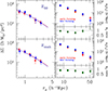 |
Fig. 1. Weak lensing (more specifically, the excess surface mass density, left) and clustering (right) measurements as a function of projected distance for clusters split in half by z50 (upper panels) and zmah (lower panels). The red and blue symbols represent early- and late-forming clusters, respectively. There are 323 and 311 early- and late-forming clusters when split by z50, div = 0.521, while 316 and 318 clusters when split by zmah, div = 0.469. WL masses for these samples are all very close, about 1.5 × 10¹⁴ h−1 M⊙ (the curves in the left panels show the best-fit models). The green points in the lower right panel are the ratio of the early-to-late wp measurements, which is equivalent to the large-scale bias ratio bearly/blate. The signature of AB at cluster scales is manifested by bearly/blate < 1, which is consistent with our measurements. The probability for these samples to be drawn from the same parent sample is p = 0.0258 (for the z50-selected samples) and p = 0.0295 (for the zmah-selected ones). |
where we and wl are shorthands for wp, early and wp, late, respectively, C is the covariance matrix built from the ratio between wp, early and wp, late and their associated jackknife samples, and constant ξ = 1. The errorbars of the wp ratio shown in Fig. 1 (as well as in Figs. 2 and 3) are calculated based on the diagonal terms of the covariance matrix C. With χ2 = 9.3 from 3 degrees of freedom, over the scales from 12.9 h−1 Mpc to 32.5 h−1 Mpc (hereafter the “mid-range”), we find that the two samples have a probability p = 0.0258 to be drawn from the same parent population (i.e., having the same large-scale bias). Using the full scale as shown in the figure (8.2 h−1 Mpc to 51.5 h−1 Mpc), the probability changes to p = 0.0393.
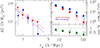 |
Fig. 2. Similar to Fig. 1, but for the z20ex, Mz set, which is selected to lie within the parameter space log M200m/(h−1 M⊙) = 14 − 14.5 and z = 0.06 − 0.12. It consists of 138 oldest (with z20 > 1.35; red solid points) and 121 youngest (with z20 < 0.85; blue solid points) clusters, with masses within 1σ of each other (the curves in the left panel show the best-fit models); the probability for the two cluster samples to have the same large-scale bias is p = 1.03 × 10⁻¹⁰ using the clustering measurements in the mid-range. In the upper right panel we show the projected correlation function of the Elucid halos that correspond to the clusters in the z20ex, Mz set (namely the counterpart halos) as open pentagons, and that of the early- and late-forming Elucid halos selected from nearly the same halo mass range to have identical mean masses (≈1.25 × 10¹⁴ h−1 M⊙; the equal mass halos – open triangles). While the clustering amplitudes of the latter are similar to the z20ex, Mz set, those of the counterpart halos deviate from the real clusters at scales larger than 30 h−1 Mpc. The early-to-late forming relative biases of the z20ex, Mz set, the counterpart halos, and the equal mass halos, are shown in the lower right panel as the green solid points, open pentagons, and open triangles, respectively. For both types of open symbols in the right panels, the horizontal locations are slightly offset from the actual values, for the sake of clarity. The error bars are obtained from the covariance matrix constructed from 400 jackknife resamples for all our clustering measurements. |
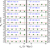 |
Fig. 3. Ratio of wp, early/wp, late = bearly/blate of the 14 control samples. The pairs are arranged in increasing masses (from top left to bottom left, continuing from top right to bottom right). In each panel, the red horizontal dashed line denotes the theoretically expected bias ratio rb, th (in the absence of AB); the 3 numbers shown in blue are the masses of the early-analogous and late-analogous clusters (in unit of 1014 h−1 M⊙), and the probability for the pair to be drawn from the same parent population. |
A similar result using cluster samples defined by zmah is shown in the lower panels of Fig. 1. The mean masses of 316 early-forming and 318 late-forming clusters are M200m = (1.52 ± 0.23)×1014 h−1 M⊙ and (1.46 ± 0.21)×1014 h−1 M⊙, respectively. Using Eq. (2), we find that the two samples have a probability p = 0.0295 (0.0152) to be consistent using the measurements from the mid-range (full-scale).
We then further seek stronger signals by exploring the extremal of the age distribution. However, as pointed out by Chue et al. (2018), at the mass scale of our clusters (i.e., around 1014 h−1 M⊙), z50 may not be the best age indicator. Quantities such as z20 or z80 may better reflect the formation history.
3.2. Age extremum selection of clusters
After testing with various age indicators mentioned above, it is found that, by selecting 138 oldest clusters with z20 > 1.35, paired with 121 youngest clusters with z20 < 0.85, both limited in the redshift range z = 0.06 − 0.12 and mass range log M200m/(h−1 M⊙) = 14 − 14.5 (as estimated by Y07), an AB-like signal can be seen. The mean masses based on WL are measured to be  and
and  , consistent within 1σ (Figs. 2 and 4). While the dividing redshifts are chosen so that we have at least 120 clusters in each sample, the redshift and halo mass ranges are selected to facilitate consistent cluster mass estimates. We shall refer to this pair of cluster samples as the z20ex, Mz set. We note in passing that the mean masses based on Y07 are (1.51 ± 0.50)×1014 h−1 M⊙ and (1.66 ± 0.55)×1014 h−1 M⊙ for the early- and late-forming samples, respectively. In Tables 1 and 2 we provide some basic information of the early- and late-forming cluster samples, respectively, which include cluster ID, cluster mass based on Y07, cluster center taken from the Y07 catalog, redshift, and z20. Given the mass difference between the early- and late-forming clusters, we should compare the measured bearly/blate to the theoretically expected bias ratio rb, th = 1.11 (assuming no effects from AB, as obtained by the bias–halo mass relation of Tinker et al. 2010), in order to evaluate the probability that the two samples have the same large-scale bias. We thus set ξ = rb, th in Eq. (2), and find the probabilities to be p = 1.02 × 10⁻¹⁰ and 1.16 × 10⁻¹¹ using the data from the mid-range and full scale, respectively.
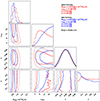 |
Fig. 4. Corner plot showing 1σ and 2σ (darker and lighter colored, respectively) confidence levels of our measurements and the nuisance parameters (qcen and αcen; see Sect. 2.4) for the z20ex, Mz set. While we can confidently constrain the cluster masses (e.g., top left panel), the constraining power on the total mass concentration is unfortunately weak (top panel in the second column from the left). |
Early-forming clusters of the z20ex, Mz set.
Late-forming clusters of the z20ex, Mz set.
We note that the mean masses of the Elucid halos that correspond to the early- and late-forming clusters are (1.36 ± 0.69)×1014 h−1 M⊙ and (1.62 ± 0.77)×1014 h−1 M⊙, respectively. We shall refer to these halos as the counterpart halos. While the WL mass of the early-forming cluster sample is close to the mean mass of the counterpart halos, the situation is different for the late-forming clusters and their associated halos. Not only do the masses differ (at 1.5 − 2σ level), the sign is also changed between the observed and simulated samples (in the z20ex, Mz set, the late-forming cluster sample has a lower mean mass than the early-forming ones, opposite to the simulated halos). We show the ratio of PCCFs of early-to-late-forming halos as open pentagons in the lower right panel of Fig. 2. Although the ratios are similar to that of the z20ex, Mz set, we note that the actual amplitude of clustering (i.e., the absolute values of bias) of the counterpart halos differ somewhat from the real clusters at scales larger than 30 h−1 Mpc (see the open pentagons in the upper right panel). The PCCFs of the counterpart halos are obtained by cross correlating these halos with low mass halos in the mass range log M200m/(h−1 M⊙) = 11.5 − 12.52. To make an accurate comparison of the resulting wp, early, co and wp, late, co of the counterpart halos with those of the z20ex, Mz set, we also cross correlate the observed clusters with the same set of low mass halos in Elucid, and multiply wp, early, co and wp, late, co with a factor ζ that makes the amplitudes of the z20ex, Mz cluster–halo PCCF and the z20ex, Mz cluster–SDSS galaxy PCCF at 8.2 h−1 Mpc identical.
Given the relatively large uncertainties in the WL mass measurements of the z20ex, Mz set, we have to test their effects on the AB signal exhibited by our cluster samples, by considering an extreme case where the differences in the large-scale clustering are maximally due to the cluster mass difference. To do so, we consider two cases: (1) assuming that the mean mass of the early-forming cluster sample is biased high by 1σ, while that of the late-forming one is biased low by 1σ, and (2) assuming that the mean mass of the late-forming sample is biased low by at least 2σ. While there is a 2.6% probability for the first case to occur, the likelihood for the second case is 2.3%. For the first case, we set ξ = rb, th to 0.92, the value corresponding to the bias ratio of halos of masses M200m, early, min = 0.97 × 10¹⁴ h−1 M⊙ (i.e., 1σ lower than the mean mass of the early-forming clusters) and M200m, late, max = 1.21 × 10¹⁴ h−1 M⊙ (1σ higher than the mean mass of the late-forming clusters) in Eq. (2). In the calculation above, we have again used the bias–halo mass relation of Tinker et al. (2010), and set ξ = rb, th in Eq. (2). Using the mid-range (full scale) clustering measurements, we find that the probability for the pair of cluster samples to have the same bias becomes p = 7.49 × 10⁻⁵ (5.40 × 10⁻⁵). As for the second case, we keep the mass of the early-forming sample at the measured value, while increase the mean mass of the late-forming one to 1.47 × 10¹⁴ h−1 M⊙. The expected bias ratio is rb, th = 0.94, which is high compared to our measurements. The probabilities are p = 2.44 × 10⁻⁵ and 1.35 × 10⁻⁵ using the mid-range and full scale data, respectively.
However, if we take into account the potential uncertainties of in the theoretical predictions of the bias ratio from Tinker et al. (2010), and artificially decrease rb, th by 10%, the probabilities become 5.30 × 10⁻³ and 4.53 × 10⁻³ (for case 1) 2.50 × 10⁻³ and 2.13 × 10⁻³ (for case 2) using the mid-range and full scale data, respectively; these correspond to significance levels of 2.8σ (case 1) and 3σ (case 2).
In the upper (lower) right panel of Fig. 2, we further show the theoretically expected PCCFs (bearly/blate ratio) as the open triangles, as derived from Elucid, in which the effect of AB must be present. We first select dark matter halos with masses M200m = (0.7 − 1.9)×1014 h−1 M⊙, then separate them into early- and late-forming using the same redshift division as done for the z20ex, Mz set. This pair of halos will be referred to as the equal mass halos. We then cross-correlate the resulting 98 early-forming and 82 late-forming halos, which have mean masses of (1.24 ± 0.31)×1014 h−1 M⊙ and (1.26 ± 0.36)×1014 h−1 M⊙, respectively, with low mass halos in the mass range log M200m/(h−1 M⊙) = 11.5 − 12.5, and derive the ratio between wp, early, eq and wp, late, eq. The triangles appear to be consistent with our measurements (the solid points), indicating that the AB signal from the z20ex, Mz set is similar in amplitude to that expected in ΛCDM. The probability for the early- and late-forming halos to have the same large-scale bias is p = 1.78 × 10⁻⁴ using the mid-range clustering measurements. Similar to the PCCFs of the counterpart halos, the PCCFs of the equal mass halos (shown as open triangles in the upper right panel of Fig. 2) have been adjusted in amplitude by the same factor ζ.
We conclude by noting that, while the mean masses and mass ranges of the counterpart halos and equal mass halos differ, both exhibit a similar degree of AB. Therefore, despite the WL mass uncertainties of the z20ex, Mz set, if AB exists in the real Universe at the predicted amplitude, the signal should still be detectable.
3.3. Galaxy properties of the z20ex, Mz set
We next examine various properties related to cluster galaxy populations in the z20ex, Mz set. We first measure the stacked galaxy surface density profiles of the early- and late-forming clusters. Fitting the density profiles of red galaxies with r-band absolute magnitudes of −24 ≤ Mr ≤ −18 with an NFW model, we find concentration values of  (with reduced
  with 16 degrees of freedom) and
  (
( ), which are consistent with the expectation that early-forming clusters would have a more spatially concentrated galaxy population, a premise of the analysis of M16. Despite having a 33% higher mean cluster mass, the early-forming clusters are found to have 25% fewer galaxies (of all colors) than the late-forming ones. Given the halo occupation number measured from a sample of nearby clusters, one expects the cluster galaxy number
  (Lin et al. 2004); this makes the “deficit” of galaxies in our early-forming sample to be about 60% compared to the case when AB does not play a role. Such a reduction in member galaxy number could be due to that, for an older cluster population, cluster galaxies are subject to dynamical processes such as tidal stripping for a longer time and can lose mass (and fade in luminosity as they age) and fall below our detection limit (e.g., Zentner et al. 2005). In addition, there is also longer time for dynamical friction to drive more galaxies to the center and merge with the BCG.
One rough way to examine whether a cluster is relaxed or not is to check the proximity of its BCG to the center. In the Y07 catalog, the cluster center is a luminosity weighted mean from all member galaxies. We have calculated the distances of BCGs from the cluster center for the z20ex, Mz set, finding that BCGs in the early- and late-forming samples have a median separation from the center of de = (0.11 ± 0.01) r200m and dl = (0.14 ± 0.01) r200m, respectively. Such off-center values are consistent with our prior employed in the WL analysis (Sect. 2.4), and are consistent with the expectation that older clusters would have BCGs closer to their center.
We further examine the formation time of the cluster galaxy properties, particularly the BCGs, using results from the full spectral fitting code STARLIGHT (Cid Fernandes et al. 2013) as well as the spectral energy distribution fitting technique presented in Chang et al. (2015). We do not find any appreciable differences in the ages of member galaxies in the early- and late-forming clusters, which might be due to the combination of (1) small cluster sample size, (2) insufficient depth of SDSS photometry and spectra, and the theoretical expectation that cluster galaxies have formed most of their stars prior to becoming members of the clusters we observe (e.g., Guo et al. 2011; for old stellar populations, it is extremely difficult to detect any age differences using tools currently available).
Finally, we investigate the magnitude gap Δ12 of the z20ex, Mz set, which is the differences in the r-band absolute magnitudes between the BCG and the second most luminous galaxy (Tremaine & Richstone 1977). Additionally, we also examine Δ14, the magnitude difference between the BCG and the fourth most luminous galaxy, as it has been suggested to be a more robust measure of the gap (Golden-Marx & Miller 2018). Using the cluster member catalog of Y07, we find that the median Δ12 = 0.44 ± 0.01 (Δ14 = 0.99 ± 0.01) with a scatter of 0.05 for the early-forming clusters, while that of the late-forming clusters is Δ12 = 0.38 ± 0.01 (Δ14 = 0.87 ± 0.01) with a scatter of 0.05. These results are again consistent with the expectation that the gap increases as a cluster ages, as more and more massive satellites are cannibalized by the BCG via dynamical friction (Ostriker & Tremaine 1975).
To summarize, for this pair of cluster samples, we find from the properties of cluster galaxy populations evidence supporting their age differences, including (1) higher concentration of spatial distribution of red galaxies, (2) significantly reduced total galaxy number, (3) smaller offset of BCGs from cluster center, and (4) larger magnitude gap, when comparing early-forming clusters with the late-forming ones.
3.4. Null tests
As a sanity check, we construct 14 pairs of control cluster samples that have similar distributions in halo mass and redshift as the z20ex, Mz set, but chosen from the parent cluster sample regardless of their z20, to demonstrate the robustness of our method. These samples are generated in the following way (and will be referred to as the control samples hereafter). We first make grids in the M − z space limited to that spanned by the z20ex, Mz set, that is, log M200m/(h−1 M⊙) = 14 − 14.5 and z = 0.06 − 0.12. To generate a control sample analogous to the early-forming clusters of the z20ex, Mz set, we only select clusters from grids in which the number of clusters from the full sample (of 634 clusters) is at least more than two larger than the number of early-forming clusters from the z20ex, Mz set. A late-forming cluster sample analog is generated in a similar fashion. We note that the early-analog and late-analog samples are generated independently of each other.
In Fig. 3 we show the ratio wp, early/wp, late = bearly/blate of the control samples. Each pair consists of 138 early-analog and 121 late-analog clusters, identical to that of the z20ex, Mz set. In the upper left part of each panel, we show the masses of the early-analogous and late-analogous clusters as measured via stacked WL (in unit of 1014 h−1 M⊙), and the probability for the pair to be drawn from the same parent population (using the clustering measurements within the mid-range). The red horizontal line denotes the bias ratio expected (in the absence of AB) given the masses of the cluster samples in consideration. As we arrange the pairs in increasing masses, the red line is always very close to unity (shown as the black dotted line). None of these shows probabilities as low as that of the z20ex, Mz set.
For these 14 pairs of cluster samples, we have fit an NFW profile to the spatial distribution of member galaxies. For each pair, which by design have similar masses, we compute the ratio of the measured concentration parameters (early-analog over late-analog), as well as that of the total number of member galaxies. The mean ratio and standard deviation of concentration are found to be (1.19, 0.24), while those of the total galaxy number are (0.90, 0.13); the scatters of these quantities are comparable to those from the literature (about 15% for concentration and 30% for galaxy number, e.g., Lin et al. 2004; Hennig et al. 2017), thus we can regard both quantities to be consistent with unity, indicating that these pairs of cluster samples have galaxy properties largely consistent with each other. Furthermore, we note that the mean separations between the BCG and cluster center are (0.20 ± 0.01) r200m and (0.22 ± 0.01) r200m for the early- and late-analog samples, respectively.
Finally, the median magnitude gaps are found to be Δ12 = 0.42 ± 0.01 (Δ14 = 0.99 ± 0.01) for the 14 early-forming analog cluster samples (with a scatter of 0.05), while those for the late-forming analog ones are Δ12 = 0.42 ± 0.01 (Δ14 = 0.97 ± 0.01), also with a scatter of 0.05. These smaller magnitude gaps, as compared to those of our zz20ex, Mz set (cf. the values reported in the penultimate paragraph of Sect. 3.3), provide further support that the formation time derived from Elucid is informative.
4. Discussion
As our z20ex, Mz set is constructed using the halo formation time from Elucid, some readers may wonder whether we are measuring the AB signal in Elucid or in the real Universe. A related concern is, would it be circular to use a CDM-based simulation (which must contain the AB signal) to infer the halo formation time, and in turn use it to construct the cluster samples.
In simplest terms, we can recast our study as a hypothesis test, with the ultimate goal of ruling out the null hypothesis that the real Universe has no AB. Thinking of this problem in a Bayesian way, we have
 (3)
(3)
where “AB” stands for “AB exists in the Universe”, “data” refers to properties of our z20ex, Mz set (including WL mass, clustering measurements, as well as cluster galaxy properties), and the prior P(AB|Elucid) should be taken to be uninformative, say 50% chance for P(AB|Elucid) = 1 or 0. As for the likelihood P(data|AB, Elucid), logically, we can consider four general cases that result from the combination of (1) whether there is AB in the real Universe (which is assumed to be described by the ΛCDM model3), and (2) whether there is AB in Elucid, and compare our observational findings (presented in Sects. 3.3 and 3.4) with the predicted observational results to deduce in which of the four cases we are in.
First of all, we do see a strong signal of AB in Elucid (i.e., the open triangles in the lower right panel of Fig. 2), so we can rule out two of the four possible cases. Then the main issue is to determine whether our data also requires AB to be present in the real Universe. To answer this question, let us refer to Table 3, where in the first column we list four observables we have presented in Sect. 3.3, and in subsequent columns we list in turn the expected behavior when there is AB in the Universe, our observed trends, the behavior when we are seeing an AB-like signal simply because of any potential circularity in our methodology, and the behavior when such a signal is simply due to an incorrect cluster mass estimation (that is, for example, the mass of our late-forming cluster sample is underestimated by at least 2σ, which has a 2.3% chance to occur; please see Sect. 3.2).
Expected observational signatures of various possibilities of AB detection.
In a Universe where there is AB, we expect that the early-forming clusters to have a higher mass concentration than their late-forming counterparts, when their masses are the same. Given that our WL measurements could not provide adequate constraints (Fig. 4), we have to resort to the spatial distribution of cluster galaxies. Assuming the red galaxy distribution follows that of the matter (e.g., Adhikari et al. 2021), we then expect to have ce > cl. As for the number of member galaxies N, it is expected that N in early-forming clusters should be smaller than that in the late-forming ones (see our argument at the end of the first paragraph in Sect. 3.3), resulting in Ne < Nl. Similarly, in older clusters, the BCGs are expected to be closer to the center (hence de < dl), and have a larger magnitude gap (yielding Δe > Δl). These expectations are all consistent with what we have observed with the z20ex, Mz set, shown in the third column.
In the fourth column, we show the expectation for the case where we are simply measuring AB in Elucid, and that AB does not exist in the real Universe (let us for the moment allow for such an inconsistency with ΛCDM). By “circularity”, we mean that, given the density field Elucid was tasked to reconstruct is based on the groups and clusters from the Y07 catalog, the Elucid halos are naturally expected to be located in large-scale environments (then indirectly, bias) similar to the real clusters used in our analysis. In such a case, the formation time indicator we use (z20) is only meaningful for the Elucid halos and has nothing to do with the real clusters4; for all four observables, they should therefore be similar (or identical) for the early- and late-forming clusters, since they have similar (or identical) masses. The different behavior of the observables from the expectation shown in the second column provides evidence against the notion that we are measuring AB in the simulation. It is important to note that our cross-correlation function measurements rely primarily on the spatial distribution of the SDSS main galaxy sample, which is far below the spatial resolution of Elucid, so our measurements are not purely based on Elucid. Another point worth noting is that the halo mass estimates from Y07 may not be accurate even in the cluster regime. This is not only reflected in the late-forming sample of the z20ex, Mz set, but also the wide range of halo masses of our control sample clusters: recall that in Sect. 3.4, these samples are all chosen to have similar Y07 halo mass distribution as the z20ex, Mz set. It is thus highly nontrivial that z20 from Elucid can be used to split the real clusters into early- and late-forming ones that exhibit an AB-like signature5.
Finally, in the fifth column, we consider the case where an AB-like signal arises due to a significant underestimation of the mass of our late-forming cluster sample. Given the weak-to-no dependence on cluster mass of the observed total cluster galaxy concentration (e.g., Lin et al. 2004; Hennig et al. 2017), we thus expect ce ≈ cl for the cluster mass range we consider (i.e., from ≈0.9 to 2 × 10¹⁴ h−1 M⊙). For the galaxy number, given the observed trend that  with a scatter of about 30% (Lin et al. 2004), it is expected that Ne ≲ Nl, although it could easily be Ne ≳ Nl given the scatter in the N − M relation. We caution that the concentration and galaxy number derived from photometric galaxy data could suffer from projection effects (caused by large-scale structures along the line of sight; e.g., Zu et al. 2017; Sunayama & More 2019), and therefore one has to be careful in interpreting these results. We note that our cluster samples are based on spectroscopic redshifts, so the identification of clusters (and their member galaxies) is not affected by projection effects.
For the BCG offset, from our control sample that contains 28 cluster samples with WL mass measurements, we see a clear trend of a decreasing offset with increasing cluster mass, and thus de > dl is expected. Finally, the magnitude gap is found to decrease with cluster mass (e.g., Yang et al. 2008; Lin et al. 2010), so we have Δe > Δl. Comparing the expectations shown in this column with those shown in the second column, we see that the main distinction comes from the BCG offset. Given that the mean values of the observed de and dl of the zz20ex, Mz set differs at 3σ level, and are far smaller than those of the control samples, we believe this feature is robust; taking into account the observed behavior of the galaxy concentration and galaxy number, it is unlikely that what we have observed is due to incorrect mass estimation.
It is worth noting that none of the 14 pairs of control samples passes these observational tests. Finally, we recall that even if the mean cluster mass of our late-forming sample is severely underestimated, the difference in the bias is still far from sufficient to explain the large difference in the large-scale biases of the early- and late-forming samples (Sect. 3.2), strongly hinting at the presence of some AB-like mechanisms at work.
In conclusion, although we construct the z20ex, Mz set using the formation history from a constrained simulation, not directly observed halo properties, seeing both the AB-like large-scale bias ratio and the consistent trends of cluster galaxy properties requires AB to not only exist in Elucid but also in the real Universe.
5. Summary and prospects
Using a novel approach of combining a constrained simulation of the local universe Elucid with a sample of galaxy clusters from SDSS, we have constructed a pair of early- and late-forming cluster samples. The formation time indicator z20 of the clusters is derived from their counterpart massive halos found in Elucid. While WL-based cluster mass estimates indicate the two samples are comparable (within 1σ), their large-scale biases differ significantly, which imply the presence of AB (with the correct sign that older clusters are less biased than the younger ones). Furthermore, the properties of the galaxy populations of the two samples are also consistent with the expectation of the age difference: the early-forming clusters have a more concentrated red galaxy surface density profile, much smaller number of member galaxies, smaller offset of BCGs from cluster center, and a larger magnitude gap, compared to the late-forming ones. The signal is found to be consistent with the theoretical prediction of ΛCDM, which is remarkable given that there is no guarantee that the formation time of halos from Elucid would match that of the real clusters. In the unlikely (∼2.5% chance) case where the differences in clustering measurements are largely due to the cluster mass difference, and take into account of possible uncertainties in the theoretical predictions of large-scale bias, our cluster samples still exhibit an AB-like signal at ≈3σ level.
Our analysis can also be regarded as a hypothesis test – based on the extensive discussion presented in Sect. 4, we can rule out the null hypothesis that the real Universe has no AB at 99.7% confidence level. Our z20ex, Mz set would be invaluable for further studies of aspects related to AB, such as the measurements of the splashback radius (e.g., More et al. 2016), pressure profile of the intracluster medium, the BCG-to-total stellar mass ratio, etc. Furthermore, the member galaxy properties of our cluster samples can serve as foundations for a natural extension of our pursuit toward a more empirical detection of AB, namely to use cluster samples purely constructed from observables. One can devise ways to split clusters of similar masses into old and young ones based on the combination of spatial distribution of member galaxies, member galaxy number, BCG offset, and magnitude gap. To minimize projection effects, it is desirable to use large cluster samples built by spectroscopic redshifts (e.g., Y07, Tinker 2021).
Forward-modeling techniques like the one used to construct Elucid, as well as BORG (Jasche & Wandelt 2013), TARDIS (Horowitz et al. 2019), COSMIC BIRTH (Kitaura et al. 2021), are gaining increasing popularity (e.g., Nguyen et al. 2020; Tsaprazi et al. 2022; Ata et al. 2022), and they have immense potential for advancing our understanding of structure formation. In this study we have demonstrated that a pair of cluster samples exhibiting a probable AB signal can be constructed using Elucid. With Elucid, in principle we can further study AB manifested in other halo properties such as spin or concentration. Furthermore, Yang et al. (2018) have also used Elucid to develop the neighborhood abundance matching method. Finally, with rich spectroscopic data coming from surveys like Dark Energy Spectroscopic Instrument (DESI; DESI Collaboration 2016) and Subaru Prime Focus Spectrograph (PFS; Takada et al. 2014; Greene et al. 2022), one can expect the reconstruction to become much more reliable, particularly at higher redshifts (e.g., Ata et al. 2022), which would facilitate studies of AB in the distant universe.
To enhance the legacy value of Elucid, with this paper we make the Elucid data publicly available6.
Choosing a smaller matching radius (e.g., 3 h−1 Mpc) and a more strict mass ratio constraint (e.g., |log(M1/M2)| < 0.3) would result in 540 matches. For our main cluster samples (to be presented in Sect. 3.2), the reduction of sample size is around 80%, with very similar halo mass distributions, and thus will not change our conclusions.
With coordinates of all halos transformed from the (x, y, z) space of Elucid to (RA, Dec, redshift) space first.
Given that AB is an important feature of ΛCDM, this phenomenon should naturally exist in the Universe. One may then ask what the point is of carrying out the analysis presented in this paper. Firstly, having a measurement that is consistent with a theoretical prediction is an important step in scientific analyses. A prime example is the black hole shadow images obtained by the Even Horizon Telescope Collaboration (Event Horizon Telescope Collaboration 2019; Akiyama et al. 2022), which spectacularly confirm the predictions of General Relativity. Secondly, to cite one of the most famous experiments in cosmology, to detect the baryon acoustic oscillation (BAO) signal, one needs to first assume the CDM framework is correct, then proceed to convert the BAO scale from an angular to a physical one (e.g., Eisenstein et al. 2005).
In principle, z20 from Elucid may still trace the formation history of the real clusters, but cluster properties in the real Universe would not be correlated with the formation time given that there is no AB in the Universe.
Despite the observational evidence, one might still argue, regarding any potential circularity in our methodology, that if we were to randomly shuffle z20 among the Elucid halos, while all the large-scale structures in the local Universe are still preserved, we would not be able to see the AB signal. We believe such an argument is flawed, as a modified Elucid with randomized halo formation history would violate the basic constraints of the CDM model of cosmology (or likely any sensible models of structure formation): the time continuity of the density field would be broken, and the spatial power spectrum and high-order statistics would be incorrect at any epochs other than z = 0.
Acknowledgments
We are grateful to Huiyuan Wang for providing data from the Elucid simulation, and Rachel Mandelbaum for sharing the SDSS shape catalog. We thank an anonymous referee for comments that have improved the clarity of the paper. We appreciate helpful comments from Ue-Li Pen, Zheng Zheng, Yao-Yuan Mao, Huiyuan Wang, Xiaohu Yang, Houjun Mo, Eiichiro Komatsu, Yen-Chi Chen, Benedikt Diemer, Andrey Kravtsov, Neal Dalal, and You-Hua Chu. Y.T.L. is supported by the National Science and Technology Council of Taiwan under grants MOST 111-2112-M-001-043, MOST 110-2112-M-001-004, and MOST 109-2112-M-001-005, and a Career Development Award from Academia Sinica (AS-CDA-106-M01). H.M. is supported by World Premier International Research Center Initiative, MEXT, and JSPS KAKENHI Grant Numbers JP20H01932 and JP21H05456. H.G. is supported by NSFC (Nos. 11922305, 11833005). T.W.L. is supported by the MOST 111-2112-M-002-015-MY3, the Ministry of Education, Taiwan (Yushan Young Scholar grant NTU-110VV007), National Taiwan University research grant (NTU-CC-111L894806). Y.T.L. thanks I.H., L.Y.L. and A.L.L. for constant encouragement and inspiration. Funding for the SDSS and SDSS-II has been provided by the Alfred P. Sloan Foundation, the Participating Institutions, the National Science Foundation, the US Department of Energy, the National Aeronautics and Space Administration, the Japanese Monbukagakusho, the Max Planck Society, and the Higher Education Funding Council for England. The SDSS WebSite is http://www.sdss.org/. The SDSS is managed by the Astrophysical Research Consortium for the Participating Institutions. The Participating Institutions are the American Museum of Natural History, Astrophysical Institute Potsdam, University of Basel, University of Cambridge, Case Western Reserve University, University of Chicago, Drexel University, Fermilab, the Institute for Advanced Study, the Japan Participation Group, Johns Hopkins University, the Joint Institute for Nuclear Astrophysics, the Kavli Institute for Particle Astrophysics and Cosmology, the Korean Scientist Group, the Chinese Academy of Sciences (LAMOST), Los Alamos National Laboratory, the Max-Planck-Institute for Astronomy (MPIA), the Max-Planck-Institute for Astrophysics (MPA), New Mexico State University, Ohio State University, University of Pittsburgh, University of Portsmouth, Princeton University, the United States Naval Observatory, and the University of Washington.
References
- Abazajian, K. N., Adelman-McCarthy, J. K., Agüeros, M. A., et al. 2009, ApJS, 182, 543 [Google Scholar]
- Akiyama, K., Alberdi, A., Alef, W., et al. 2022, ApJ, 930, L12 [NASA ADS] [CrossRef] [Google Scholar]
- Adhikari, S., Shin, T.-H., Jain, B., et al. 2021, ApJ, 923, 37 [NASA ADS] [CrossRef] [Google Scholar]
- Ata, M., Lee, K.-G., Vecchia, C. D., et al. 2022, Nat. Astron., 6, 857 [NASA ADS] [CrossRef] [Google Scholar]
- Baldry, I. K., Glazebrook, K., Brinkmann, J., et al. 2004, ApJ, 600, 681 [Google Scholar]
- Blanton, M. R., Schlegel, D. J., Strauss, M. A., et al. 2005, AJ, 129, 2562 [NASA ADS] [CrossRef] [Google Scholar]
- Chang, Y.-Y., van der Wel, A., da Cunha, E., & Rix, H.-W. 2015, ApJS, 219, 8 [Google Scholar]
- Chue, C. Y. R., Dalal, N., & White, M. 2018, JCAP, 2018, 012 [Google Scholar]
- Cid Fernandes, R., Pérez, E., García Benito, R., et al. 2013, A&A, 557, A86 [NASA ADS] [CrossRef] [EDP Sciences] [Google Scholar]
- Conroy, C., Wechsler, R. H., & Kravtsov, A. V. 2006, ApJ, 647, 201 [Google Scholar]
- Contreras, S., Chaves-Montero, J., Zennaro, M., et al. 2021, MNRAS, 507, 3412 [NASA ADS] [CrossRef] [Google Scholar]
- DESI Collaboration (Aghamousa, A., et al.) 2016, ArXiv e-prints [arXiv:1611.00036] [Google Scholar]
- Eisenstein, D. J., Zehavi, I., Hogg, D. W., et al. 2005, ApJ, 633, 560 [Google Scholar]
- Event Horizon Telescope Collaboration (Akiyama, K., et al.) 2019, ApJ, 875, L1 [Google Scholar]
- Feldmann, R., Carollo, C. M., Porciani, C., et al. 2006, MNRAS, 372, 565 [NASA ADS] [CrossRef] [Google Scholar]
- Gao, L., Springel, V., & White, S. D. M. 2005, MNRAS, 363, L66 [NASA ADS] [CrossRef] [Google Scholar]
- Golden-Marx, J. B., & Miller, C. J. 2018, ApJ, 860, 2 [NASA ADS] [CrossRef] [Google Scholar]
- Greene, J., Bezanson, R., Ouchi, M., et al. 2022, ArXiv e-prints [arXiv:2206.14908] [Google Scholar]
- Guo, H., Li, C., Zheng, Z., et al. 2017, ApJ, 846, 61 [NASA ADS] [CrossRef] [Google Scholar]
- Guo, Q., White, S., Boylan-Kolchin, M., et al. 2011, MNRAS, 413, 101 [Google Scholar]
- Hennig, C., Mohr, J. J., Zenteno, A., et al. 2017, MNRAS, 467, 4015 [NASA ADS] [Google Scholar]
- Hirata, C., & Seljak, U. 2003, MNRAS, 343, 459 [Google Scholar]
- Horowitz, B., Lee, K.-G., White, M., et al. 2019, ApJ, 887, 61 [NASA ADS] [CrossRef] [Google Scholar]
- Jasche, J., & Wandelt, B. D. 2013, MNRAS, 432, 894 [Google Scholar]
- Jing, Y. P., Suto, Y., & Mo, H. J. 2007, ApJ, 657, 664 [NASA ADS] [CrossRef] [Google Scholar]
- Kitaura, F.-S., Ata, M., Rodríguez-Torres, S. A., et al. 2021, MNRAS, 502, 3456 [NASA ADS] [CrossRef] [Google Scholar]
- Komatsu, E., Dunkley, J., Nolta, M. R., et al. 2009, ApJS, 180, 330 [NASA ADS] [CrossRef] [Google Scholar]
- Lan, T.-W., Ménard, B., & Mo, H. 2016, MNRAS, 459, 3998 [NASA ADS] [CrossRef] [Google Scholar]
- Landy, S. D., & Szalay, A. S. 1993, ApJ, 412, 64 [Google Scholar]
- Lin, Y.-T., Mohr, J. J., & Stanford, S. A. 2004, ApJ, 610, 745 [NASA ADS] [CrossRef] [Google Scholar]
- Lin, Y.-T., Ostriker, J. P., & Miller, C. J. 2010, ApJ, 715, 1486 [Google Scholar]
- Lin, Y.-T., Mandelbaum, R., Huang, Y.-H., et al. 2016, ApJ, 819, 119 [NASA ADS] [CrossRef] [Google Scholar]
- Mandelbaum, R., Hirata, C. M., Seljak, U., et al. 2005, MNRAS, 361, 1287 [Google Scholar]
- Mandelbaum, R., Hirata, C. M., Leauthaud, A., Massey, R. J., & Rhodes, J. 2012, MNRAS, 420, 1518 [NASA ADS] [CrossRef] [Google Scholar]
- Mandelbaum, R., Slosar, A., Baldauf, T., et al. 2013, MNRAS, 432, 1544 [NASA ADS] [CrossRef] [Google Scholar]
- Mansfield, P., & Kravtsov, A. V. 2020, MNRAS, 493, 4763 [NASA ADS] [CrossRef] [Google Scholar]
- Mao, Y.-Y., Zentner, A. R., & Wechsler, R. H. 2018, MNRAS, 474, 5143 [NASA ADS] [CrossRef] [Google Scholar]
- Miyatake, H., More, S., Takada, M., et al. 2016, Phys. Rev. Lett., 116, 041301 [NASA ADS] [CrossRef] [Google Scholar]
- More, S., Miyatake, H., Takada, M., et al. 2016, ApJ, 825, 39 [NASA ADS] [CrossRef] [Google Scholar]
- Nakajima, R., Mandelbaum, R., Seljak, U., et al. 2012, MNRAS, 420, 3240 [NASA ADS] [Google Scholar]
- Navarro, J. F., Frenk, C. S., & White, S. D. M. 1997, ApJ, 490, 493 [Google Scholar]
- Nguyen, N.-M., Jasche, J., Lavaux, G., et al. 2020, JCAP, 2020, 011 [CrossRef] [Google Scholar]
- Oke, J. B., & Gunn, J. E. 1983, ApJ, 266, 713 [NASA ADS] [CrossRef] [Google Scholar]
- Ostriker, J. P., & Tremaine, S. D. 1975, ApJ, 202, L113 [NASA ADS] [CrossRef] [Google Scholar]
- Reyes, R., Mandelbaum, R., Gunn, J. E., et al. 2012, MNRAS, 425, 2610 [NASA ADS] [CrossRef] [Google Scholar]
- Rykoff, E. S., Rozo, E., Busha, M. T., et al. 2014, ApJ, 785, 104 [Google Scholar]
- Springel, V., White, S. D. M., Jenkins, A., et al. 2005, Nature, 435, 629 [Google Scholar]
- Strauss, M. A., Weinberg, D. H., Lupton, R. H., et al. 2002, AJ, 124, 1810 [Google Scholar]
- Sunayama, T., & More, S. 2019, MNRAS, 490, 4945 [NASA ADS] [CrossRef] [Google Scholar]
- Takada, M., & Jain, B. 2003a, MNRAS, 340, 580 [NASA ADS] [CrossRef] [Google Scholar]
- Takada, M., & Jain, B. 2003b, MNRAS, 344, 857 [Google Scholar]
- Takada, M., Ellis, R. S., Chiba, M., et al. 2014, PASJ, 66, R1 [Google Scholar]
- Tinker, J. L. 2021, ApJ, 923, 154 [NASA ADS] [CrossRef] [Google Scholar]
- Tinker, J. L., Robertson, B. E., Kravtsov, A. V., et al. 2010, ApJ, 724, 878 [NASA ADS] [CrossRef] [Google Scholar]
- Tinker, J. L., Cao, J., Alpaslan, M., et al. 2021, MNRAS, 505, 5370 [NASA ADS] [CrossRef] [Google Scholar]
- Tremaine, S. D., & Richstone, D. O. 1977, ApJ, 212, 311 [NASA ADS] [CrossRef] [Google Scholar]
- Tsaprazi, E., Nguyen, N. M., Jasche, J., et al. 2022, JCAP, 08, 003 [CrossRef] [Google Scholar]
- Wang, H., Mo, H. J., Yang, X., Jing, Y. P., & Lin, W. P. 2014, ApJ, 794, 94 [NASA ADS] [CrossRef] [Google Scholar]
- Wang, H., Mo, H. J., Yang, X., et al. 2016, ApJ, 831, 164 [Google Scholar]
- Wang, W., & White, S. D. M. 2012, MNRAS, 424, 2574 [Google Scholar]
- Wechsler, R. H., & Tinker, J. L. 2018, ARA&A, 56, 435 [NASA ADS] [CrossRef] [Google Scholar]
- Wechsler, R. H., Zentner, A. R., Bullock, J. S., Kravtsov, A. V., & Allgood, B. 2006, ApJ, 652, 71 [NASA ADS] [CrossRef] [Google Scholar]
- Yang, X., Mo, H. J., van den Bosch, F. C., et al. 2007, ApJ, 671, 153 [Google Scholar]
- Yang, X., Mo, H. J., & van den Bosch, F. C. 2008, ApJ, 676, 248 [Google Scholar]
- Yang, X., Zhang, Y., Wang, H., et al. 2018, ApJ, 860, 30 [NASA ADS] [CrossRef] [Google Scholar]
- York, D. G., Adelman, J., Anderson, J. E., Jr., et al. 2000, AJ, 120, 1579 [NASA ADS] [CrossRef] [Google Scholar]
- Zentner, A. R., Berlind, A. A., Bullock, J. S., et al. 2005, ApJ, 624, 505 [NASA ADS] [CrossRef] [Google Scholar]
- Zu, Y., Mandelbaum, R., Simet, M., Rozo, E., & Rykoff, E. S. 2017, MNRAS, 470, 551 [CrossRef] [Google Scholar]
- Zu, Y., Shan, H., Zhang, J., et al. 2021, MNRAS, 505, 5117 [CrossRef] [Google Scholar]
All Tables
All Figures
|
Fig. 1. Weak lensing (more specifically, the excess surface mass density, left) and clustering (right) measurements as a function of projected distance for clusters split in half by z50 (upper panels) and zmah (lower panels). The red and blue symbols represent early- and late-forming clusters, respectively. There are 323 and 311 early- and late-forming clusters when split by z50, div = 0.521, while 316 and 318 clusters when split by zmah, div = 0.469. WL masses for these samples are all very close, about 1.5 × 10¹⁴ h−1 M⊙ (the curves in the left panels show the best-fit models). The green points in the lower right panel are the ratio of the early-to-late wp measurements, which is equivalent to the large-scale bias ratio bearly/blate. The signature of AB at cluster scales is manifested by bearly/blate < 1, which is consistent with our measurements. The probability for these samples to be drawn from the same parent sample is p = 0.0258 (for the z50-selected samples) and p = 0.0295 (for the zmah-selected ones). |
| In the text | |
|
Fig. 2. Similar to Fig. 1, but for the z20ex, Mz set, which is selected to lie within the parameter space log M200m/(h−1 M⊙) = 14 − 14.5 and z = 0.06 − 0.12. It consists of 138 oldest (with z20 > 1.35; red solid points) and 121 youngest (with z20 < 0.85; blue solid points) clusters, with masses within 1σ of each other (the curves in the left panel show the best-fit models); the probability for the two cluster samples to have the same large-scale bias is p = 1.03 × 10⁻¹⁰ using the clustering measurements in the mid-range. In the upper right panel we show the projected correlation function of the Elucid halos that correspond to the clusters in the z20ex, Mz set (namely the counterpart halos) as open pentagons, and that of the early- and late-forming Elucid halos selected from nearly the same halo mass range to have identical mean masses (≈1.25 × 10¹⁴ h−1 M⊙; the equal mass halos – open triangles). While the clustering amplitudes of the latter are similar to the z20ex, Mz set, those of the counterpart halos deviate from the real clusters at scales larger than 30 h−1 Mpc. The early-to-late forming relative biases of the z20ex, Mz set, the counterpart halos, and the equal mass halos, are shown in the lower right panel as the green solid points, open pentagons, and open triangles, respectively. For both types of open symbols in the right panels, the horizontal locations are slightly offset from the actual values, for the sake of clarity. The error bars are obtained from the covariance matrix constructed from 400 jackknife resamples for all our clustering measurements. |
| In the text | |
|
Fig. 3. Ratio of wp, early/wp, late = bearly/blate of the 14 control samples. The pairs are arranged in increasing masses (from top left to bottom left, continuing from top right to bottom right). In each panel, the red horizontal dashed line denotes the theoretically expected bias ratio rb, th (in the absence of AB); the 3 numbers shown in blue are the masses of the early-analogous and late-analogous clusters (in unit of 1014 h−1 M⊙), and the probability for the pair to be drawn from the same parent population. |
| In the text | |
|
Fig. 4. Corner plot showing 1σ and 2σ (darker and lighter colored, respectively) confidence levels of our measurements and the nuisance parameters (qcen and αcen; see Sect. 2.4) for the z20ex, Mz set. While we can confidently constrain the cluster masses (e.g., top left panel), the constraining power on the total mass concentration is unfortunately weak (top panel in the second column from the left). |
| In the text | |
Current usage metrics show cumulative count of Article Views (full-text article views including HTML views, PDF and ePub downloads, according to the available data) and Abstracts Views on Vision4Press platform.
Data correspond to usage on the plateform after 2015. The current usage metrics is available 48-96 hours after online publication and is updated daily on week days.
Initial download of the metrics may take a while.