| Issue |
A&A
Volume 666, October 2022
|
|
|---|---|---|
| Article Number | A61 | |
| Number of page(s) | 13 | |
| Section | Interstellar and circumstellar matter | |
| DOI | https://doi.org/10.1051/0004-6361/202243441 | |
| Published online | 10 October 2022 | |
Eclipse of the V773 Tau B circumbinary disc★,★★
1
Leiden Observatory, University of Leiden,
PO Box 9513,
2300 RA
Leiden, The Netherlands
e-mail: This email address is being protected from spambots. You need JavaScript enabled to view it.
2
Department of Physics and Astronomy, Wayne State University,
666 W Hancock St,
Detroit, MI
48201, USA
3
Department of Physics and Astronomy, University of Nevada,
Las Vegas,
4505
South Maryland Parkway, NV
89154,
USA
4
Department of Physics and Astronomy, Michigan State University,
East Lansing, MI
48824, USA
5
Department of Physics, University of Warwick,
Coventry
CV4 7AL, UK
6
Astrophysikalisches Institut und Universitäts-Sternwarte Jena,
Schillergäßchen 2,
07745
Jena, Germany
7
Instituto de Física y Astronomía, Facultad de Ciencias, Universidad de Valparaíso,
Av. Gran Bretaña 1111,
Playa Ancha, Valparaíso, Chile
8
Centro de Astronomía (CITEVA), Universidad de Antofagasta,
Avenida U. de Antofagasta,
02800
Antofagasta, Chile
9
Munnerlyn Astronomical Instrumentation Laboratory, Department of Physics and Astronomy, Texas A&M university,
College Station, TX
77843, USA
Received:
28
February
2022
Accepted:
14
June
2022
Abstract
Context. Young multiple stellar systems can host both circumstellar and circumbinary discs composed of gas and dust, and the orientations of circumbinary discs can be sculpted by the orientation and eccentricity of the central binaries. Studying multiple binary systems and their associated discs enables our understanding of the size and distribution of the planetary systems that subsequently form around them.
Aims. A deep (~70%) and extended (~150 days) eclipse was seen towards the young multiple stellar system V773 Tau in 2010. We interpret it as being due to the passage of a circumbinary disc around the B components moving in front of the A components. Our aim is to characterise the orientation and structure of the disc, to refine the orbits of the sub-components, and to predict when the next eclipse will occur.
Methods. We combined the photometry from several ground-based surveys, constructed a model for the light curve of the eclipse, and used high angular resolution imaging to refine the orbits of the three spatially resolved components of the system: A, B, and C. A frequency analysis of the light curves, including from the TESS satellite, enabled the characterisation of the rotational periods of the Aa and Ab stars.
Results. A toy model of the circumbinary disc shows that it extends out to approximately 5 au around the B binary and has an inclination of 73° with respect to the orbital plane of AB, where the lower bound of the radius of the disc is constrained by the geometry of the AB orbit and the upper bound is set by the stability of the disc. We identify several frequencies in the photometric data that we attribute to rotational modulation of the Aa and Ab stellar companions. We produced the first determination of the orbit of the more distant C component around the AB system and limited its inclination to 93°.
Conclusions. The high inclination and large diameter of the disc, together with the expected inclination of the disc from theory, suggest that B is an almost equal-mass, moderately eccentric binary. We identify the rotational periods of the Aa and Ab stars and a third frequency in the light curve that we attribute to the orbital period of the stars in the B binary. We predict that the next eclipse will occur around 2037, during which both detailed photometric and spectroscopic monitoring will characterise the disc in greater detail.
Key words: (stars:) binaries: general / eclipses / protoplanetary disks
Processed photometric data and light curves are only available at the CDS via anonymous ftp to cdsarc.u-strasbg.fr (130.79.128.5) or via http://cdsarc.u-strasbg.fr/viz-bin/cat/J/A+A/666/A61
The manuscript and processing scripts are available in a GitHub repository at https://github.com/mkenworthy/V773TauBdisk
© M. A. Kenworthy et al. 2022
 Open Access article, published by EDP Sciences, under the terms of the Creative Commons Attribution License (https://creativecommons.org/licenses/by/4.0), which permits unrestricted use, distribution, and reproduction in any medium, provided the original work is properly cited.
This article is published in open access under the Subscribe-to-Open model. This email address is being protected from spambots. You need JavaScript enabled to view it. to support open access publication.
1 Introduction
Young multiple stellar systems are common (e.g. Ghez et al. 1993; Duchêne & Kraus 2013), as are gas discs in and around the stellar components (Akeson et al. 2019). Chaotic accretion can occur during the star formation process as a result of turbulence within the molecular cloud from which the stars form (Bate et al. 2003; McKee & Ostriker 2007). Circumstellar and circumbinary discs can form with a misalignment to the binary orbital plane (Monin et al. 2007; Bate 2018).
These binaries have been shown to influence and sculpt the circumbinary discs around them, possibly reinvigorating planet formation (Cabrit et al. 2006; Rodriguez et al. 2018). The torque from a binary or multiple stellar system affects the formation and evolution of gas discs (e.g. Nelson 2000; Mayer et al. 2005; Boss 2006; Fu et al. 2017) and the interaction between planets and the disc (Picogna & Marzari 2015; Lubow & Martin 2016; Martin et al. 2016). Thus, understanding how stellar multiplicity affects the formation and evolution of discs is important to explain observed exoplanet properties.
A misaligned circumbinary disc undergoes retrograde nodal precession. If the binary is in a circular orbit, the precession is always around the binary angular momentum vector (e.g. Larwood et al. 1996). However, around an eccentric binary the precession is around the binary eccentricity vector if the initial misalignment is sufficiently high (Farago & Laskar 2010; Aly et al. 2015). Dissipation within the disc causes it to align coplanar to the binary orbit, or polar to the binary orbit and aligned with the binary eccentricity vector (Martin & Lubow 2017; Lubow & Martin 2018; Zanazzi & Lai 2018). While all currently detected circumbinary planets are in coplanar orbits, around an eccentric binary polar planets may be more stable than coplanar planets (Chen et al. 2020), and terrestrial planets at least form more efficiently (Childs & Martin 2021). If the disc’s lifetime is shorter than its alignment timescale then planets may form in misaligned orbits.
There are now many observations of circumbinary discs with a range of misalignment angles. For example, KH 15D has a misalignment of about 3–15° (Chiang & Murray-Clay 2004; Winn et al. 2004; Capelo et al. 2012; Poon et al. 2021). IRS 43 is misaligned by more than 60° (Brinch et al. 2016), and the circumbinary disc around 99 Her has a polar misalignment (Kennedy et al. 2012). HD 98800 has a misalignment of 90°, meaning it is polar aligned to the central binary orbit (Kennedy et al. 2019; Zúñiga-Fernández et al. 2021). Of the two possible disc inclinations allowed by observations, the polar alignment was first suggested by considering the dynamics of a disc since the polar alignment timescale is short compared to the stellar age. Furthermore, the size of the inner hole in the disc that is carved by the binary orbit (Artymowicz & Lubow 1994) is in agreement with a polar alignment (Franchini et al. 2019). There is also an external binary companion to the circumbinary disc in this system, and its orbit is close to 34° to the normal of the disc’s angular momentum.
V773 Tau is a young multiple stellar system that has been intensively studied as described in Sect. 2. It contains three components, each at a distinctly different stage of young stellar evolution – the A component is an almost equal-mass binary, which in itself orbits around an almost equal-mass B component that has disc around it, forming a hierarchical multiple system with a decades-long orbit. Both these components are orbited by a third, C component that is highly embedded within a cloud of dust and is on a several-hundred-year orbit around both A and B.
In Sect. 3, we present the photometry of the V773 system from several ground-based surveys. A deep extended eclipse occurs over a 200-day period, and we attribute this to a disc around the B component passing in front of the A components. This disc is highly inclined with respect to the AB orbital plane, which should otherwise become coplanar within a dynamically short timescale. Previous work (Boden et al. 2012) indicates that the B component is itself a tight, almost equal-mass binary system. If the B binary is also eccentric, then the disc will experience a torque that keeps it at the inclination that we observe. Time series analysis of the photometry reveals two rotational periods consistent with the stars in the A binary, and a third period of approximately 67 days is revealed in the analysis. If this period is attributed to the orbital period of the B binary, we show that a moderate orbital eccentricity will keep the circumbinary disc at the observed inclination. We derive the properties of the B binary and the circumbinary disc, and in Sect. 4 use the astrometry from the direct imaging observations to determine the expected epoch of the next eclipse of the A system.
Section 5 details our analysis of the photometric fluctuations due to rotational modulation of both Aa and Ab, and it identifies a photometric signal whose period is a plausible measure of the orbit of the BaBb binary. The long and extended eclipse is modelled in Sect. 6 as an azimuthally symmetric dusty disc that is highly inclined to the AB orbital plane. Theoretical consideration of the torques from an eccentric binary on a surrounding disc are discussed in Sect. 7 along with the prediction for the timing of the next eclipse in Sect. 8. We summarise our results and discuss future observations in Sect. 9.
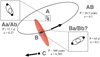 |
Fig. 1 Sketch of V773 Tau system. We hypothesise that B is itself an equal-mass binary system with a moderately eccentric orbit. Orbits are not to scale. |
2 The V773 Tau system
2.1 Discovery and architecture
V773 Tau (HD 283447, HBC 367) is a young (3 ± 1 Myr; Boden et al. 2007) stellar system that was identified as a young T Tauri star (Rydgren et al. 1976) and subsequently resolved as a visual double system (Ghez et al. 1993; Leinert et al. 1993). Its age was determined by comparing the temperature and luminosity of the stars Aa and Ab with pre-main sequence (PMS) stellar models from Montalbán & D’Antona (2006), which show excellent consistency with the component parameters from Boden et al. (2007). It is located at a distance of 132.8 ± 2.3 pc as determined by orbital and trigonometric parallax (Torres et al. 2012), in contradiction with the larger distance determined by Gaia EDR3. We attribute this discrepancy to the multiple-source nature of the system that is not resolved by Gaia, and we use the distance determined by the spatially resolved A components with the VLA observations (Torres et al. 2012).
The bound components of V773 Tau were initially identified as A, B, and C (see Fig. 1). The A component was resolved by Very Long Baseline Array observations to be a binary system with PAaAb = 51.1003 ± 0.0022 days and an eccentricity of e = 0.2710 ± 0.0072 (Torres et al. 2012). The A binary becomes more luminous in radio waves during the periastron passage of the A stars, which is thought to be from the interacting magnetic fields of the two stars (Torres et al. 2012).
A is orbited by the B component over a period of approximately 26 yr, and both A and B are orbited by a C component with an orbital period of several hundred years (Duchêne et al. 2003). C is a heavily reddened companion that is the faintest component at a wavelength of two microns but is the brightest at 4.7µm (Duchêne et al. 2003; Woitas 2003). The flux contribution from C at optical wavelengths is approximately 100 times fainter than the A and B components (Duchêne et al. 2003).
2.2 The B component
Photometry of the B component shows a significantly greater amount of extinction compared to the A component, implying the presence of additional dust along the line of sight to the B component (Torres et al. 2012). The Β component shows significant photometric variability of the order of 2–3 magnitudes in the Κ band (Boden et al. 2012), which is consistent with clouds or clumps of dust orbiting around the Β component. The initial fit to the spectral energy distribution (SED) suggested that the Β component consisted of a single Κ star (Duchêne et al. 2003), but subsequent radial velocity monitoring and astrom-etry of the A binary enabled a dynamical mass determination of both the Β and A components, revealing a much larger mass of 2.35 M⊙ for the Β component (Boden et al. 2012). A single 2.35 M⊙ star would have a luminosity of 17 L⊙, which is inconsistent with the optical luminosity observed and the extinction derived. If the Β system is itself a binary, BaBb, then assuming equal-mass components of 1.5 M⊙ yields a much lower luminosity that is consistent with the observed SED, see Table 2 for a summary of the parameters we adopt. We therefore assume that the V773 Tau AB system is a hierarchical quadruple system, with a circumbinary disc around the Β component that is responsible for the significant reddening and photometric variability seen in its vicinity.
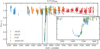 |
Fig. 2 Optical photometry of V773 Tau system. The four different photometric surveys are represented by different colours, and each photometric series has been normalised using flux outside the main eclipse. The inset panel shows the eclipse light curve in greater detail. The PTF and KELT curves show different depths of the eclipse, indicating the presence of sub-micron dust that causes different amounts of optical extinction in the different pass bands of the two surveys. |
3 Data
3.1 Discovery of the Eclipse with KELT
The Kilodegree Extremely Little Telescope (KELT; Pepper et al. 2007, 2012, 2018) survey is a project searching for transiting exoplanets, using two robotic wide-field telescopes, one at the Winer Observatory in Arizona (KELT-N) and the Southern African Astronomical Observatory (SAAO) near Sutherland (KELT-S). The observatories consist of a 4096 × 4096 AP16E Apogee CCD camera (KELT-N) and 4096 × 4096 Alta U16M Apogee CCD camera (KELT-S) using a Kodak Wratten #8 red-mass filter, comparable to an R band magnitude. The cameras are fed with a ƒ/19 42 mm (wide angle survey mode with 26° × 26° field of view) or a ƒ/28 200 mm (narrow angle campaign mode with 10.8° × 10.8° field of view) Mamiya lenses. Images are obtained at a cadence of 10–30 min and yield useful magnitudes from 7 to 13.
The KELT survey has been highly successful in the discovery and analysis of systems being eclipsed by circumstellar material, including the longest period eclipsing binary (Rodriguez et al. 2016). To search for eclipses of YSOs, we cross-matched the Zari et al. (2018) catalogue of young stars in the solar neighbourhood that were identified by a combination of Gaia DR2 (Gaia Collaboration 2018) photometry and kinematics with the KELT catalogue to obtain a sample of ~1450 stars with light curves. The corresponding KELT light curves for each YSO target were visually inspected for any large dimming events (> 10%) that lasted more than a week. From this analysis, we identified an ~80% deep dimming event in V773 Tau, which is shown in Fig. 2. The eclipse is incomplete, with the first half of the eclipse occurring when V773 Tau was behind the Sun, so we only observed the egress of the eclipse that lasted ~100 days. Based on this discovery, we searched for the eclipse in other photometric data sets.
3.2 ASAS
The All Sky Automated Survey (ASAS; Pojmanski 1997, 2005; Simon et al. 2018) is a survey consisting of two observing stations – one in Las Campanas, Chile and the other on Maui, Hawaii. Each observatory is equipped with two CCD cameras using V and I filters and commercial ƒ = 200 mm, D = 100 mm lenses, although both larger (D = 250 mm) and smaller (50–72 mm) lenses were used at earlier times. The majority of the data were taken with a pixel scale of ≈15″. ASAS splits the sky into 709 partially overlapping (9° × 9° fields, taking on average 150 3-min exposures per night, leading to a variable cadence of 0.3–2 frames per night. Depending on the equipment used and the mode of operation, the ASAS limiting magnitude varied between 13.5 and 15.5 mag in V, and the saturation limit was 5.5 to 7.5 mag. Precision is around 0.01–0.02 mag for bright stars and below 0.3 mag for the fainter ones. ASAS photometry is calibrated against the Tycho catalogue, and its accuracy is limited to 0.05 mag for bright, non-blended stars.
3.3 ASAS-SN
The All Sky Automated Survey for Supernovae (ASAS-SN; Shappee et al. 2014; Kochanek et al. 2017) consists of six stations around the globe, with each station hosting four telescopes with a shared mount. The telescopes consist of a 14-cm aperture tele-photo lens with a field of view of approximately 4.5° × 4.5° and an 8.0″ pixel scale. Two of the original stations (one in Hawaii and one in Chile) are fitted with V band filters, whereas the other stations (Chile, Texas, South Africa and China) are fitted with g band filters. ASAS-SN observes the whole sky every night with a limiting magnitude of about 17 mag in the V and g bands.
3.4 PTF
The Palomar Transient Factory (PTF) is an automated wide field optical photometric survey described in Law et al. (2009). It uses an 8.1 square degree camera with 101 megapixels at 1″ sampling mounted on the 48 in. Samuel Oschin telescope at the Palomar Observatory. Nearly all of the images are taken in one of two filters – Mould-R and SDSS-g′, reaching  and mR ≈ 20.6 in 60 s exposures. Over 120 photometric observations were obtained using the R band filter (Ofek et al. 2012).
3.5 TESS
The Transiting Exoplanet Survey Satellite (TESS; Ricker et al. 2015) is a satellite designed to survey for transiting exoplanets among the brightest and nearest stars over most of the sky. The TESS satellite orbits the Earth every 13.7 days on a highly elliptical orbit, scanning a sector of the sky spanning 24° × 96° for a total of two orbits, before moving on to the next sector. It captures images at two-second (used for guiding), 20-s (for 1000 bright asteroseismology targets), 120-s (for 200 000 stars that are likely planet hosts), and 30-min (full frame image) cadences. The instrument consists of four CCDs each with a field of view of 24° × 24°, a wide band-pass filter from 600 to 1000nm (similar to the IC band), and a limiting magnitude of about 14–15 mag (IC). The data were extracted from the TESS archive using the eleanor package (Feinstein et al. 2019), which corrected for known systematics in the cameras and telescope.
3.6 Combined light curve
A summary of all the photometry obtained for V773 Tau is shown in Table 3. Photometric data from each survey are normalised to account for camera and instrumental throughput offsets. The relative flux is computed for each subset of points, where the baseline is determined by ignoring in-eclipse data. The data out of eclipse are resampled to 1-day bins to improve the signal-to-noise ratio and reduce the number of points for display and analysis. Photometric outliers are removed by sigma-clipping on the flux and rejecting points with large photometric error values. Further processing includes removing the rotational variability due to the presence of spots on the A components, which was removed for each survey by fitting a stellar variability model (see Sect. 5).
The light curve of V773 Tau is shown in Fig. 2 with the photometry from all four ground-based surveys. The depth of the eclipse is approximately 80% at MJD 55450, with an estimated full width at half minimum of approximately 100 days. The start of the eclipse was not observed due to the observing season for the star. Three surveys show the eclipse, with the PTF survey showing a slightly shallower eclipse depth compared to the ASAS light curve. The PTF observed V773 Tau in the R band while ASAS observations were in the V band; as a result, there is a colour depth difference due to the wavelength-dependent nature of dust absorption, indicating sub-micron-sized dust. The data from TESS are shown in Fig. 8.
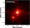 |
Fig. 3 SPHERE image of V773 Tau AB and C. The axes are centred on A, and Β is not visible in this image as it is under the first diffraction ring of the A component. C is shown to the lower left of AB. North is up and east to the left. |
3.7 Adaptive optics imaging
The V773 Tau system was observed with the SPHERE/IRDIS (Infra-Red Dual Imaging and Spectrograph; Beuzit et al. 2019; Dohlen et al. 2008), mounted at the Nasmyth platform of the Unit 3 telescope (UT3) at ESO’s VLT on 2021 Oct 28 (MJD 59515). The IRDIS camera was used to obtain 16 images with 16-s integration in direct imaging mode with no coronagraphs for a total integration time of 256 s. The astrometric PSF extraction was done by simultaneously fitting two elliptical Moffat functions to the flux image. The official astrometric calibration for the BB–K filter (Maire et al. 2016) was used to correct the observations. The image was corrected for geometric distortions and the true north offset (see Fig. 3). For the parallactic angle the header values of the data were used. Four independent measurements of the PA and separation were made (left and right detector sides, beginning and end of the sequence). The resultant position is listed in Table 4.
To confirm the astrometry of AC and to measure the AB separation in the presence of A′s diffraction rings, a custom fitting routine was used. The centre of A and C was determined by choosing a trial value for the (x, y) position of the light centroid of the stellar PSF, then rotating by 180° and subtracting this image from the unrotated image. The emcee package (Foreman-Mackey et al. 2013) was then used to minimise the calculated χ2 of the residuals within a disc with a diameter equal to that of the Airy disc of the PSF centred on the trial coordinates, and the pixel positions along with the errors derived through marginalisation of the distributions were calculated.
With the centroid of star A determined, we then subtracted a 180-degree-rotated image of A from the original image, revealing the B system at the location of the first diffraction ring of system A (see Fig. 4, left panel). We then used star C as a reference PSF, translated it to the location of B, scale the flux of the image by a factor f and then use emcee to determine the relative separation of B and C (see Fig. 4, right panel). With the absolute pixel positions of A and C, the relative position of B with respect to C and the pixel scale of the SPHERE IRDIS camera, the position angles and separations of AB and AC are determined. The AC values are found to be consistent with the Moffat fitting procedure for AC, and all fitting results are listed in Table 4.
Errors reported on the astrometry using emcee are smaller than those reported in previous measurements on larger telescopes, even though our signal-to-noise ratio is similar. The fitting routine does not include systematic errors, which are difficult to quantify with the diffraction ring residuals seen at the location of the B component. We therefore doubled the errors on the measured relative position of A from B, which is consistent with the errors reported by other papers, to represent the systematic errors in our fitting.
Orbital parameters for A and B systems.
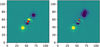 |
Fig. 4 Determining astrometry of V773 Tau A, B, and C. The left hand panel shows the rotation-subtracted image of the V773 system, which was constructed by rotating the image by 180 degrees around the centroid of A (indicated by the red dot) and then subtracting it from the original image. The positive flux image of C is seen to the lower left and the negative flux image of C to the upper right. The positive flux image of the B component is then seen to the upper right of the centroid of A, indicating its location. The right hand panel shows the subtraction of the positive image of C from the location of B, with B marked with a red circle. Residuals from the subtraction processes can be seen around the location of A and B. |
Physical parameters for V773 Tau A–B.
Summary of the photometric data for V773 Tau employed in this work.
4 Orbital fitting for A, B, and C
We combined previously obtained astrometry of the V773 Tau system (from the analysis of Duchêne et al. 2003; Boden et al. 2012) with our reported astrometry and used the orbitize! (Blunt et al. 2020; Foreman-Mackey et al. 2013) package to perform an updated orbital fit for the AB system and the orbit of C around the barycentre of AB. For orbitize!, we use 1000 walkers, 20 temperatures (to move walkers out of local minima in the optimization function), a burn in of 2000 per walker, and a total run of 106 steps for both systems. The output is in the form of orbits (consisting of six orbital elements, the total mass of the system, and the parallax) with fits consistent with the astrometry, which are referred to as a ‘bundle’. By marginalising over all the other orbital parameters in the bundle, a distribution for each orbital parameter is constructed. The value and quoted errors for the orbital elements are at the 16th, 50th, and 84th percentile points of each distribution and show no significant correlation for the AB system, indicating a good orbital fit. The orbital elements of the AB system are shown in Table 1.
With the updated orbital bundles generated for the AB system, we then took the measured AC astrometry as reported in Table 1 of Duchêne et al. (2003) and Table 1 of Boden et al. (2012) and combined it with the 2021 astrometry. We then corrected the AC relative astrometry using the measured masses of A and Β and calculated the distance from C to the barycentre of AB (called C-AB). Using the C-AB astrometry, we carried out an orbitize! fit with parameters identical to those of the AB system (see Figure 6). The orbital period of C around the AB system is of the order of hundreds of years, and so only a short arc of the orbit is traced out across the observed epochs. The resultant orbital bundle shows a much wider spread of orbital parameters, ranging from periods of several decades to almost a thousand years. The orbital bundle includes the combined mass of AB and C, including some unphysically low masses, so we keep bundles with masses between 3.5 and 7.0 M⊙.
There is, however, the matter of orbital stability within a hierarchical triple, and we can approximate the Tau system with A and Β forming an inner binary and C the distant third component orbiting them. Using the approximations within Eggleton & Kiseleva we can calculate a lower limit for the periastron of C around the AB system, and then reject orbits from the orbital bundle produced from our fitting procedure. This stability criteria is able to predict the stability over timescales of 5 × 10⁵ PAB (He & Petrovich which is much longer than the age of the system. With qin MA/MB = 1.24 and qout ≥ 7.5 and aAB 15.3 au and eAB = 0.1 this yields  and using Eq. (2) from Eggleton & Kiseleva we can derive a lower limit for the periastron distance of C. Trial masses for C vary from 0.4 to 0.7 M⊙ and only weakly change the periastron distance for C, so we set it at 68 au. After removing orbits with periastron distances smaller than this, we used this new bundle of orbits as the starting point for a second optimisation run. The resultant orbital bundles show convergence, and the triangle plot of the eccentricity and inclination of the orbit of C are very well constrained, as shown in Fig. 7. Most notably, the inclination of C is 97 + 1° with a tightly constrained eccentricity of 0.40. The asymmetry of the errors on the orbital elements reflect the wide range of possible orbits as shown in Table 1.
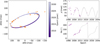 |
Fig. 5 Orbit of V773 Tau AB system. A is fixed at the origin in the left hand panel. The right hand panels show the separation and position angles of the astrometry. |
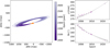 |
Fig. 6 Orbit of V773 Tau C system. The barycentre of AB is fixed at the origin in the left hand panel. The right hand panels show the separation and position angles of the astrometry. |
Orbital measurements for A, B, and C.
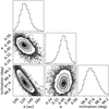 |
Fig. 7 Correlation between semi-major axis, eccentricity, and orbital inclination of the V773 Tau C system. |
5 Rotational modulation and stellar activity
The V773 Tau system was observed by TES S in Sector 19 corresponding to MJD 58816 to 58842. Several sinusoidal variations are seen in the light curve, with a total peak-to-valley variation of up to 10%, as seen in Fig. 8. A Lomb-Scargle periodogram reveals four dominant frequencies in the power spectrum, with periods of 1.29, 2.62, 1.54, and 3.09 days. Both stars are magnetically active, so it is reasonable to assume that there are multiple star spots present across their surfaces. When combined with the rotation of the star, this leads to variations in observed flux as the spots rotate in and out of view. We therefore interpret these periods as due to the rotational periods of 2.62 and 3.09 days for the stars Aa and Ab, respectively. Since these variations are not pure sinusoids, this modulation appears at double the frequencies (half the periods) in the periodogram (see Fig. 9).
Rotation periods of the order of a few days are consistent with stellar evolution models at the age of the system, around 3 Myr. Spectroscopic observations of chromospheric absorption lines show rotational broadening of ν sin i = 38 ± 4 km s−1 for the Aa component (Boden et al. 2007), and Welty (1995) quote velocities of 41.4 km s−1 and 41.9 km s−1 for Aa and Ab, respectively. Assuming stellar radii of 2.22 + 0.20 R⊙ and 1.74 ± 0.19 R⊙ for Aa and Ab, respectively (Boden et al. 2007), we can calculate the expected rotational velocity for the two stars - with the two periods we see in the periodogram, we obtain vAa = 36.4 ± 3.3 km s−1 and vAb = 34 ± 4 km s−1. We derive the inclination of the rotational equator for both stars: iAa = 73 ± 16° and iAb = 53 ± 11°, which, whilst not a strong constraint, are at least marginally consistent with the inclination of the AaAb orbital plane of 69°. Our assignment of the rotational periods to Aa and Ab could be incorrect – if these periods are assigned to the other star in the A system, then the star Aa has a rotational velocity equal to that of the projected rotational velocity, indicating that the star Aa is equator-on with an inclination of 90°, and Ab is much closer to pole-on. This would imply a far more dynamically misaligned system for A.
We modelled the light curve out of the eclipse as a sum of the four periods, mapped as a Fourier series of sines and cosines. After removing these four periods, there remains a smaller amplitude sinusoidal signal with a period of 2.45 days. We suggest that this is the rotational modulation for a star in the Β system, but we regard this as a somewhat tentative assignment that requires further confirmation with high spectral resolution spectroscopy to disentangle its nature.
In addition to short-term modulation (< 10 days), longer periodic signals can reveal the unknown orbital period of the Β component and identify the reported 51-day period of the A component. Periodograms of the separate surveys with the short-term frequencies removed are shown in Fig. 10. No 51 day period is seen, but there is a periodic signal at ~68 days that is clearly detected in all three photometric data sets. This suggests that we may be seeing the orbital period for the Β system, with the light curve modulation caused by the periodic change in orientation of the two stars. An eccentric polar orbit in the Β system would lift the apogee of both stars out of the midplane of the circumsec-ondary disc, and the resultant illumination change onto the upper surfaces of the disc leads to a periodic variation in the light curve of the system, and hence gives rise to the observed signal in the periodogram.
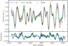 |
Fig. 8 V773 Tau light curve as observed with TESS, shown in the upper panel with brown dots. The stellar variability models computed with Lomb-Scargle (blue) and Markov chain Monte Carlo (green) are overlapped, and the residuals are indicated as a colour scale. |
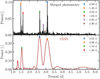 |
Fig. 9 Lomb-Scargle periodograms for the merged photometry (top) and TESS (bottom); the periods with the highest powers are highlighted. |
 |
Fig. 10 Lomb–Scargle periodograms for the two bands of ASAS-SN and KELT. In grey (green), we show the periodogram before (after) removing the short-term rotational frequencies. A peak at ~68 days is highlighted for the three data sets. |
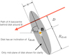 |
Fig. 11 Sketch of the disc around B. The component A passes behind the disc with a projected chord length of w. Only the midplane of the disc is shown for clarity. The radius of the disc is Rdisc with an inclination to our line of sight of idisc, and the disc is tilted by θdiscº anticlockwise from due east. |
6 Disc model for the eclipse
The V773 Tau system is unresolved by the ground-based survey telescopes, and so the light curves represent the summed flux of A, B, and C. The depth of the eclipse in the visible band is approximately 80%. The amount of flux from C at optical wavelengths is less than 1% of the total flux, so we ignore the contribution of C in the photometric analysis. A depth of 80% is consistent at optical wavelengths with a complete eclipse of the Aa/Ab stellar components by an opaque occulter. The compiled photometry covers a baseline of 18 yr, and no other significant deep eclipse is seen, which rules out a dust cloud orbiting within the region of stability around the A system.
The orbit of Β is inclined at 77° to our line of sight, and at the time of the eclipse, the Β component was passing in front of the A component, close to the minimum projected separation between A and Β (coincidentally just past the epoch of periastron). We constructed a toy model of the AB system with a disc around the Β component in order to determine the possible parameters and geometry for a circumstellar disc that is consistent with the observed photometry.
Circumstellar discs typically have a flared geometry, with a scale height for the dust that increases with increasing radii as a power law of the radius (Dullemond et al. 2002). The outermost parts of the disc will also be sculpted by the interaction with the A system and the competing torques from the Β system and geometry of the AB orbit (discussed in Sect. 7), resulting in many degrees of freedom for any fit to the photometry. We simplify our model and approximate the disc as a cylindrical slab of dust with radius Rdisc with the density of dust being a function of the height above the midplane. In cylindrical coordinates, we assume the absorbing material for r < Rdisc is A(r, ϕ,z) oc z and A = 0 for r > Rdisc. If the disc is exactly edge on to the line of sight, then a single star passing behind the disc would have a light curve where the absorption is proportional to the dust absorption integrated along the line of sight from the background star to the Earth. Since we are assuming a cylindrical slab, this integrated absorption is proportional to a Gaussian distribution: A(z) = A0 exp(−(z/σdisc)2) where z is the vertical height above the midplane of the disc and σdisc is the characteristic scale height of the dust. If the disc is tilted to the line of sight, then the star crosses a chord across the midplane of the disc of projected a width w (see Fig. 11), which samples a different part of the Gaussian distribution for that region of the disc. The inclination of the disc with respect to the line of sight idisc is related to the radius and inclination of the disc by

The long axis of the projected disc is tilted at an angle θdisc° measured anticlockwise from due east, and the impact parameter for the path of A behind Β is D. Given the depth and duration of the eclipse, the extinction due to dust around Β and the projected separation of A and B, we hypothesise that the disc is nearly edge on to our line of sight.
We determine the height of the stars Aa and Ab above the midplane of the edge-on disc around the Β component by calculating the positions of the stars Aa, Ab, and Β as seen on the sky, calculating the relative positions of Aa and Ab from the Β component, and then rotating these relative positions by an angle of θdisc with the location of Β as the origin into the coordinate frame of the disc. We then calculate the height of the star above the disc as a function of time t, producing ZAa(t) and ZAb(t) and using the Gaussian function we calculate the flux of Aa and Ab through the disc a flux ratio of the two stars as F(Ab)/F(Aa).
Our model disc flux is therefore

which represents the flux for both stars transmitted through a tilted disc with projected chord width w, the scale height σdisc, and maximum absorption in the disc Amax. The inclination of the disc is a function of both w and the radius of the disc Rdisc, which itself cannot be determined from the light curve. Instead, we assumed a given radius for the disc and then used w to estimate its inclination.
We used the emcee package to perform a fit of F(t) to the photometric light curve over the epochs of the eclipse. We minimised the χ2 statistic to obtain our fit using 100 walkers and a burn in of 300 steps. From Boden et al. (2007), the flux ratio between Aa and Ab was calculated to be F(Ab)/F(Aa) = 0.37 ± 0.03 at a mean wavelength of 518 nm. As a consequence, we carried out two separate model fits. In the first case, we fixed the flux ratio at 0.37 (see Fig. 12), and in the second case we allowed the flux ratio between the two A components to be a free parameter (see Fig. 13). The fits and marginalised errors on the parameters are shown in Table 5.
A tilted disc around Β can reach an outer radius of up to 0.38 aAB, giving Rdisc = 5.24 au for e = 0.1 and an equal mass binary (see Fig. 4 from Miranda & Lai 2015). The projected separation of A and Β during the midpoint of the eclipse D = 4.78 au, and the mean velocity of Β around A as projected on the sky is 0.0111 au day−1. We calculate that the circumbinary disc is close to edge-on, approximately 10° from an edge-on geometry. An approximate measure of the flare of the disc is given by σdisc/D ≈ 0.05. Finally, the inclination of the disc with respect to the AB orbital plane can take one of two values depending on whether the light curve ingress is due to the near side or far side of the disc, but both values are around 72° inclination, strongly supporting the theory that the disc around the Β component is around a polar aligned binary with moderate eccentricity.
Parameters for the circumbinary disc model.
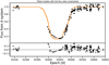 |
Fig. 12 Model with F(Aa)/F(Ab) constrained. |
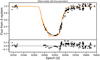 |
Fig. 13 Model with all free parameters. |
7 A tilted, polar circumbinary disc
In this section, we consider the dynamics of a circumbinary disc in this quadruple star system. In order for the stellar system to be stable, each binary must be inclined by less than about 40° to the AB binary orbital plane, otherwise the stars will undergo Kozai–Lidov (KL) oscillations of eccentricity and inclination (von Zeipel 1910; Kozai 1962; Lidov 1962). A stable circumbinary disc around stars undergoing KL oscillations is unlikely. The disc, however, is likely to be above the critical KL inclination since is it close to 90° to the AB binary orbital plane (Lubow & Ogilvie 2017; Zanazzi & Lai 2017). If the disc were orbiting a single star, it would be KL unstable (Martin et al. 2014; Fu et al. 2015a) and would move towards alignment with the AB binary orbital plane on a timescale of tens of orbital periods of the AB binary. However, the inner binary causes nodal precession that can stabilise the disc against KL oscillations (Verrier & Evans 2009; Martin et al. 2022) and lead to polar alignment in which the disc is perpendicular to the binary orbit and aligned to the eccentricity vector of the inner binary (Martin & Lubow 2017).
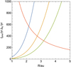 |
Fig. 14 Particle nodal precession timescale and KL timescale as a function of the particle separation from the BaBb binary. The blue (eb = 0.2), orange (eb = 0.5), and green (eb = 0.8) lines show the nodal precession timescales. The red line shows the KL timescale. The particle is unstable if the nodal precession timescale is longer than the KL timescale (Verrier & Evans 2009). |
7.1 Particle dynamics
We consider the dynamics of a test particle that orbits the BaBb binary. First, we examine the effect of the inner binary on the test particle in the absence of the outer binary. The particle is highly inclined to the inner binary orbit. It undergoes nodal precession about the eccentricity vector of the binary (Verrier & Evans 2009; Farago & Laskar 2010; Doolin & Blundell 2011; Chen et al. 2019). The frequency for the precession of a particle at semi-major axis R is given by
 (1)
(1)
where the B binary’s angular frequency is given by
 (2)
(2)
and
 (3)
(3)
(Farago & Laskar 2010; Lubow & Martin 2018). The timescale for the precession is
 (4)
(4)
We assume that the inner binary has equal mass components with a total mass of MBaBb = 2.4 M⊙. The binary orbits with a semi-major axis of aBaBb = 0.43 au. Figure 14 shows the nodal precession timescale for particles around binaries with three different eccentricities. The nodal precession timescale increases with distance from the inner binary and decreases with binary eccentricity.
In the absence of the inner binary, the outer binary component causes KL oscillations of the highly inclined test particle. These are oscillations in the eccentricity and inclination of the orbit (e.g. Naoz 2016). These occur on a timescale given by
 (5)
(5)
for a circular orbit outer binary (Kiseleva et al. 1998; Ford et al 2000), where the orbital period of the particle is  . The outer binary companion has a mass of MAaAb = 2.9 M⊙ and is in a circular orbit with a semi-major axis of aAB = 15 au. The red line in Fig. 14 shows the KL timescale.
Particles are unstable outside of the radius where the KL timescale becomes smaller than the nodal precession timescale (Verrier & Evans 2009; Martin et al. 2022). Thus, in the absence of gas, solid particles are only stable to a radius much smaller than 5 au. The larger the inner binary eccentricity, the farther out stable particles can exist. However, since the disc in V773 Tau is observed to extend to a radius of around 5 au, there must be gas present in the disc. A gas disc is in radial communication and this can allow it to be stable in a region that individual particles may be unstable.
7.2 Disc dynamics
The outer edge of the disc is likely tidally truncated by the torque from the A binary component. The outer radius of the disc decreases with the eccentricity of the AB binary (Artymowicz & Lubow 1994) and the inclination of the disc to the AB binary orbital plane (Lubow et al. 2015). The disc can extend to a radius of about 0.38 aAB when it is misaligned to the AB binary orbital plane by 90° (Miranda & Lai 2015).
If the disc is in good radial communication, it can undergo solid body precession (Larwood et al. 1996). Radial communication in the disc is maintained through pressure-induced bending waves that travel at a speed of Cs/2 (Papaloizou & Lin 1995; Lubow et al. 2002), where Cs ≈ ΗΩ is the gas sound speed. The radial communication timescale is tc ≈ 2Rout/Cs. With H/R = 0.05 and Rout = 5 au, we have tc = 47 yr. Provided that the precession is on a timescale that is significantly longer than this, then we expect solid body precession of the disc. We note that if the disc is not in good radial communication then it may undergo breaking where the disc forms disjoint rings that precess at different rates (e.g. Larwood et al. 1996; Nixon et al. 2013). This may shorten the alignment timescale (e.g. Smallwood et al. 2020).
We first ignore the A binary and consider the dynamics as a result of the inner binary. For a sufficiently high inclination, the disc’s angular momentum vector precesses about the binary eccentricity vector (Aly et al. 2015) and because viscous dissipation aligns towards this polar inclination (Martin & Lubow 2017). We consider the precession rate for the circumbinary disc as a result of the torque from the inner binary for varying inner binary separation. The inner binary carves a cavity in the inner parts of the disc. The size of the cavity depends on the binary eccentricity and the disc inclination (Artymowicz & Lubow 1994; Miranda & Lai 2015; Franchini et al. 2019). We assume that the surface density extends from an inner radius of Rin = 2.5 aBaBb out to Rout = 5 au with a profile of Σ ∝ R−3/2.
We calculated a disc-density-averaged nodal precession timescale with Eq. (16) in Lubow & Martin (2018). The blue line in Fig. 15 shows the circumbinary disc nodal precession timescale for a disc that is precessing around the BaBb binary eccentricity vector. We also calculated the disc-density-weighted KL timescale with Eq. (4) in Martin et al. (2014), and this is shown in the yellow line. The disc KL oscillation timescale is shorter than the nodal precession timescale only for small binary eccentricities. We expect that a disc may remain in a stable polar configuration for binary eccentricity eb ≳ 0.3. However, we caution that this should be verified with numerical simulations that include both binary components. While a particle that undergoes KL oscillations becomes unstable because of the high eccentricity achieved, the KL oscillations of a disc are damped and do not reach such high eccentricities (e.g. Fu et al. 2015a,b). Furthermore, disc breaking may be more likely with both an inner and an outer binary, and so an inner polar ring may still be possible even around smaller binary eccentricity (Martin et al. 2022). However, in order to have the disc out to 5 au in a polar configuration, we believe that a larger binary eccentricity is required.
We note that all of the timescales calculated in this section are approximate since we assume a truncated power-law surface density. The surface-density profile is affected by the inclination of the disc and will evolve as the disc aligns. Hydrodynamical simulations of a polar-aligning disc found that the alignment timescale was about a factor of two faster in the simulation as predicted by the linear theory (Smallwood et al. 2020). This system should be investigated in hydrodynamical simulations in the future. This would allow us to put stronger constraints on the orbital parameters of the BaBb binary.
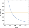 |
Fig. 15 Disc nodal precession timescale (blue) and KL timescale (orange) as a function of the eccentricity of the BaBb binary. The disc can remain polar if the nodal precession timescale is shorter than the KL timescale. |
8 Discussion
8.1 Orbital dynamics of the C component
Without radial velocity measurements, orbital fits with direct imaging have two degenerate orbital solutions. For the orbit of C around the AB system, one orbital solution has the orbital vector almost antiparallel to the orbit of the AB system (where C is in front of the AB system) at 166°. The other solution has C behind the AB system and with C orbiting in the same direction as the AB system, with a mutual inclination of 29°. If the stellar system formed from the same cloud of protostellar material, this would suggest that the inclination of 29° is the correct orbit, but radial velocity measurements of C will break this degeneracy.
8.2 The B circumbinary disc
The eclipse cannot be fit with an exactly edge-on Gaussian disc; the bottom of the eclipse is too broad with respect to the wings of the eclipse. A disc that is tilted with respect to the line of sight provides a significantly improved fit, but without a measured outer radius for the disc there is a degeneracy between the tilt of the disc and the radius. We ran two separate models for the eclipse. In the first one, we fixed the brightness ratio of the A binary at the measured value and for the second model we leave it as a free parameter – we note that the free parameter fit gives a brightness ratio for Aa and Ab that is almost exactly the opposite of that measured in previous papers. The free parameter fit had a lower χ2 value, but both models yielded similar parameters for the inclination, chord width, and scale height of the disc. Possible explanations for this include an incorrect assumption about the symmetry of the disc, especially since we are probing radii close to the outer edge of the disc, where warping from coplanar geometry is possible. Another degeneracy exists with the direction of the tilt: whether the leading edge of the eclipse is caused by the front edge or the back edge of the disc. In either possible configuration, the disc has a significant inclination of around 70° with respect to the orbital plane of AB.
8.3 The next eclipse
The resulting orbital fit bundle is shown in Fig. 5. We can see using the astrometric fit that the midpoint of the next eclipse will be on 2037 March 10, plus or minus 25 days (2037.19 ± 0.07 yr). As the next eclipse approaches, nightly photometric monitoring with the AAVSO association will alert observers to start a detailed observational campaign.
9 Conclusions
We have discovered an extended eclipse seen towards the V773 Tau multiple star system, and we hypothesise that it is due to a disc of dust orbiting the B component. In order to see the eclipse, the disc must be significantly inclined with respect to the orbital plane of the AB system, implying a restoring torque that prevents the disc from becoming coplanar with the AB orbit. The V773 Tau system has a large mid-IR flux (Prusti et al. 1992; Duchêne et al. 2003; Padgett et al. 2007) above that of the photospheric levels expected from the stellar components, and sub-millimetre flux at 850 µm and 1.3 mm (Andrews & Williams 2005) consistent with the presence of dust in the system. Due to the confounding effects of the dust around C (Duchêne et al. 2003; Woitas 2003), estimating a mass of the disc around B is not possible without spatially resolved sub-millimetre imaging to distinguish separate dust emission contributions from each source.
Several observations indicate that the B component is itself a binary system: the luminosity observed for B is consistent with that from two equal-mass components; the inclined disc can be dynamically stable if the B binary has a moderately eccentric orbit; a 67-day modulation in the light curve of the system would be consistent with a change in illumination of the circumbinary disc due to the eccentric orbital motion of the two B components in a polar orbit. We conclude that B is a moderately eccentric, nearly equal-mass binary on a 67-day orbital period with polar orientation with respect to the surrounding disc.
A direct imaging observation of the V773 Tau system enables a refinement of the orbital elements of the AB system and a first determination of the orbital elements of the AB-C system. The C system has a well-constrained inclination and eccentricity, with an orbital period from 570 to 700 yr, and it is moderately inclined (≈30°) with respect to the AB system.
The fortuitous alignment of the circumsecondary disc around V773 Tau B enables an additional characterisation of a young multiple stellar system that contains three components at different stages of evolution. An observational campaign during the next eclipse in 2037 will enable the spectroscopic characterisation of the disc, including gas and dust kinematics at scales significantly smaller than can be observed with large distributed interferometers such as the Atacama Large Millimeter/submillimeter Array.
Acknowledgements
We thank our referees for their constructive comments which helped improve this paper. This research has used the SIMBAD database, operated at CDS, Strasbourg, France (Wenger et al. 2000). This work has used data from the European Space Agency (ESA) mission Gaia (https://www.cosmos.esa.int/gaia), processed by the Gaia Data Processing and Analysis Consortium (DPAC, https://www.cosmos.esa.int/web/gaia/dpac/consortium). Funding for the DPAC has been provided by national institutions, in particular the institutions participating in the Gaia Multilateral Agreement. To achieve the scientific results presented in this article we made use of the Python programming language (Python Software Foundation, https://www.python.org/), especially the SciPy (Virtanen et al. 2020), NumPy (Oliphant 2006), Matplotlib (Hunter 2007), emcee (Foreman-Mackey et al. 2013), and astropy (Astropy Collaboration 2013, 2018) packages. We acknowledge with thanks the variable star observations from the AAVSO International Database contributed by observers worldwide and used in this research. We thank the Las Cumbres Observatory and its staff for its continuing support of the ASAS-SN project, and the Ohio State University College of Arts and Sciences Technology Services for helping us set up and maintain the ASAS-SN variable stars and photometry databases. ASAS-SN is supported by the Gordon and Betty Moore Foundation through grant GBMF5490 to the Ohio State University and NSF grant AST-1515927. Development of ASAS-SN has been supported by NSF grant AST-0908816, the Mt. Cuba Astronomical Foundation, the Center for Cosmology and AstroParticle Physics at the Ohio State University, the Chinese Academy of Sciences South America Center for Astronomy (CASSACA), the Villum Foundation, and George Skestos. Early work on KELT-North was supported by NASA Grant NNG04GO70G. Work on KELT-North was partially supported by NSF CAREER Grant AST-1056524 to S. Gaudi. Work on KELT-North received support from the Vanderbilt Office of the Provost through the Vanderbilt Initiative in Data-intensive Astrophysics. Part of this research was carried out in part at the Jet Propulsion Laboratory, California Institute of Technology, under a contract with the National Aeronautics and Space Administration (80NM0018D0004). This publication makes use of VOSA, developed under the Spanish Virtual Observatory project supported by the Spanish MINECO through grant AyA2017-84089. VOSA has been partially updated by using funding from the European Union’s Horizon 2020 Research and Innovation Programme, under Grant Agreement number 776403 (EXOPLANETS-A) The research of CA is supported by the Comité Mixto ESO-Chile and the VRIIP/DGI at the University of Antofagasta. G.M.K. is supported by the Royal Society as a Royal Society University Research Fellow. M.A.K. thanks Sarah Blunt and Jason Wang for discussions on setting up orbit bundles.
References
- Akeson, R. L., Jensen, E. L. N., Carpenter, J., et al. 2019, ApJ, 872, 158 [Google Scholar]
- Aly, H., Dehnen, W., Nixon, C., & King, A. 2015, MNRAS, 449, 65 [NASA ADS] [CrossRef] [Google Scholar]
- Andrews, S. M., & Williams, J. P. 2005, ApJ, 631, 1134 [Google Scholar]
- Artymowicz, P., & Lubow, S. H. 1994, ApJ, 421, 651 [Google Scholar]
- Astropy Collaboration (Robitaille, T.P., et al.) 2013, A&A, 558, A33 [NASA ADS] [CrossRef] [EDP Sciences] [Google Scholar]
- Astropy Collaboration (Price-Whelan, A.M., et al.) 2018, AJ, 156, 123 [NASA ADS] [CrossRef] [Google Scholar]
- Bate, M. R. 2018, MNRAS, 475, 5618 [Google Scholar]
- Bate, M. R., Lubow, S. H., Ogilvie, G. I., & Miller, K. A. 2003, MNRAS, 341, 213 [NASA ADS] [CrossRef] [Google Scholar]
- Beuzit, J. L., Vigan, A., Mouillet, D., et al. 2019, A&A, 631, A155 [NASA ADS] [CrossRef] [EDP Sciences] [Google Scholar]
- Blunt, S., Wang, J. J., Angelo, I., et al. 2020, AJ, 159, 89 [NASA ADS] [CrossRef] [Google Scholar]
- Boden, A. F., Torres, G., Sargent, A. I., et al. 2007, ApJ, 670, 1214 [NASA ADS] [CrossRef] [Google Scholar]
- Boden, A. F., Torres, G., Duchêne, G., et al. 2012, ApJ, 747, 17 [NASA ADS] [CrossRef] [Google Scholar]
- Boss, A. P. 2006, ApJ, 641, 1148 [NASA ADS] [CrossRef] [Google Scholar]
- Brinch, C., Jørgensen, J. K., Hogerheijde, M. R., Nelson, R. P., & Gressel, O. 2016, ApJ, 830, L16 [Google Scholar]
- Cabrit, S., Pety, J., Pesenti, N., & Dougados, C. 2006, A&A, 452, 897 [CrossRef] [EDP Sciences] [Google Scholar]
- Capelo, H. L., Herbst, W., Leggett, S. K., Hamilton, C. M., & Johnson, J. A. 2012, ApJ, 757, L18 [NASA ADS] [CrossRef] [Google Scholar]
- Chen, C., Franchini, A., Lubow, S. H., & Martin, R. G. 2019, MNRAS, 490, 5634 [Google Scholar]
- Chen, C., Lubow, S. H., & Martin, R. G. 2020, MNRAS, 494, 4645 [NASA ADS] [CrossRef] [Google Scholar]
- Chiang, E. I., & Murray-Clay, R. A. 2004, ApJ, 607, 913 [NASA ADS] [CrossRef] [Google Scholar]
- Childs, A. C., & Martin, R. G. 2021, ApJ, 920, L8 [NASA ADS] [CrossRef] [Google Scholar]
- Dohlen, K., Langlois, M., Saisse, M., et al. 2008, SPIE Conf. Ser., 7014, 70143L [Google Scholar]
- Doolin, S., & Blundell, K. M. 2011, MNRAS, 418, 2656 [Google Scholar]
- Duchêne, G., & Kraus, A. 2013, ARA&A, 51, 269 [Google Scholar]
- Duchêne, G., Ghez, A. M., McCabe, C., & Weinberger, A. J. 2003, ApJ, 592, 288 [CrossRef] [Google Scholar]
- Dullemond, C. P., van Zadelhoff, G. J., & Natta, A. 2002, A&A, 389, 464 [NASA ADS] [CrossRef] [EDP Sciences] [Google Scholar]
- Eggleton, P., & Kiseleva, L. 1995, ApJ, 455, 640 [NASA ADS] [CrossRef] [Google Scholar]
- Farago, F., & Laskar, J. 2010, MNRAS, 401, 1189 [Google Scholar]
- Feinstein, A. D., Montet, B. T., Foreman-Mackey, D., et al. 2019, PASP, 131, 094502 [Google Scholar]
- Ford, E. B., Kozinsky, B., & Rasio, F. A. 2000, ApJ, 535, 385 [NASA ADS] [CrossRef] [Google Scholar]
- Foreman-Mackey, D., Hogg, D. W., Lang, D., & Goodman, J. 2013, PASP, 125, 306 [Google Scholar]
- Franchini, A., Lubow, S. H., & Martin, R. G. 2019, ApJ, 880, L18 [Google Scholar]
- Fu, W., Lubow, S. H., & Martin, R. G. 2015a, ApJ, 807, 75 [NASA ADS] [CrossRef] [Google Scholar]
- Fu, W., Lubow, S. H., & Martin, R. G. 2015b, ApJ, 813, 105 [NASA ADS] [CrossRef] [Google Scholar]
- Fu, W., Lubow, S. H., & Martin, R. G. 2017, ApJ, 835, L29 [NASA ADS] [CrossRef] [Google Scholar]
- Gaia Collaboration (Brown, A.G.A., et al.) 2018, A&A, 616, A1 [NASA ADS] [CrossRef] [EDP Sciences] [Google Scholar]
- Ghez, A. M., Neugebauer, G., & Matthews, K. 1993, AJ, 106, 2005 [NASA ADS] [CrossRef] [Google Scholar]
- He, M. Y., & Petrovich, C. 2018, MNRAS, 474, 20 [NASA ADS] [CrossRef] [Google Scholar]
- Hunter, J. D. 2007, Comput. Sci. Eng., 9, 90 [NASA ADS] [CrossRef] [Google Scholar]
- Kennedy, G. M., Wyatt, M. C., Sibthorpe, B., et al. 2012, MNRAS, 421, 2264 [Google Scholar]
- Kennedy, G. M., Matrà, L., Facchini, S., et al. 2019, Nat. Astron., 3, 230 [Google Scholar]
- Kiseleva, L. G., Eggleton, P. P., & Mikkola, S. 1998, MNRAS, 300, 292 [NASA ADS] [CrossRef] [Google Scholar]
- Kochanek, C. S., Shappee, B. J., Stanek, K. Z., et al. 2017, PASP, 129, 104502 [Google Scholar]
- Kozai, Y. 1962, AJ, 67, 591 [Google Scholar]
- Larwood, J. D., Nelson, R. P., Papaloizou, J. C. B., & Terquem, C. 1996, MNRAS, 282, 597 [NASA ADS] [Google Scholar]
- Law, N. M., Kulkarni, S. R., Dekany, R. G., et al. 2009, PASP, 121, 1395 [NASA ADS] [CrossRef] [Google Scholar]
- Leinert, C., Zinnecker, H., Weitzel, N., et al. 1993, A&A, 278, 129 [NASA ADS] [Google Scholar]
- Lidov, M. L. 1962, Planet. Space Sci., 9, 719 [Google Scholar]
- Lubow, S. H., & Martin, R. G. 2016, ApJ, 817, 30 [NASA ADS] [CrossRef] [Google Scholar]
- Lubow, S. H., & Martin, R. G. 2018, MNRAS, 473, 3733 [NASA ADS] [CrossRef] [Google Scholar]
- Lubow, S. H., & Ogilvie, G. I. 2017, MNRAS, 469, 4292 [NASA ADS] [CrossRef] [Google Scholar]
- Lubow, S. H., Ogilvie, G. I., & Pringle, J. E. 2002, MNRAS, 337, 706 [NASA ADS] [CrossRef] [Google Scholar]
- Lubow, S. H., Martin, R. G., & Nixon, C. 2015, ApJ, 800, 96 [Google Scholar]
- Maire, A.-L., Langlois, M., Dohlen, K., et al. 2016, SPIE Conf. Ser., 9908, 990834 [Google Scholar]
- Martin, R. G., & Lubow, S. H. 2017, ApJ, 835, L28 [NASA ADS] [CrossRef] [Google Scholar]
- Martin, R. G., Nixon, C., Lubow, S. H., et al. 2014, ApJ, 792, L33 [Google Scholar]
- Martin, R. G., Lubow, S. H., Nixon, C., & Armitage, P. J. 2016, MNRAS, 458, 4345 [NASA ADS] [CrossRef] [Google Scholar]
- Martin, R. G., Lepp, S., Lubow, S. H., et al. 2022, ApJ, 927, L26 [NASA ADS] [CrossRef] [Google Scholar]
- Mayer, L., Wadsley, J., Quinn, T., & Stadel, J. 2005, MNRAS, 363, 641 [NASA ADS] [CrossRef] [Google Scholar]
- McKee, C. F., & Ostriker, E. C. 2007, ARA&A, 45, 565 [Google Scholar]
- Miranda, R., & Lai, D. 2015, MNRAS, 452, 2396 [Google Scholar]
- Monin, J.-L., Clarke, C. J., Prato, L., & McCabe, C. 2007, Protostars and Planets V, 395 [Google Scholar]
- Montalbán, J., & Dantona, F. 2006, MNRAS, 370, 1823 [CrossRef] [Google Scholar]
- Naoz, S. 2016, ARA&A, 54, 441 [Google Scholar]
- Nelson, A. F. 2000, ApJ, 537, L65 [Google Scholar]
- Nixon, C., King, A., & Price, D. 2013, MNRAS, 434, 1946 [NASA ADS] [CrossRef] [Google Scholar]
- Ofek, E. O., Laher, R., Law, N., et al. 2012, PASP, 124, 62 [NASA ADS] [CrossRef] [Google Scholar]
- Oliphant, T. E. 2006, A Guide to NumPy, 1 (Trelgol Publishing USA) [Google Scholar]
- Padgett, D., McCabe, C., Rebull, L., et al. 2007, in BAAS, 39, 780 [NASA ADS] [Google Scholar]
- Papaloizou, J. C. B., & Lin, D. N. C. 1995, ApJ, 438, 841 [NASA ADS] [CrossRef] [Google Scholar]
- Pepper, J., Pogge, R. W., DePoy, D. L., et al. 2007, PASP, 119, 923 [NASA ADS] [CrossRef] [Google Scholar]
- Pepper, J., Kuhn, R. B., Siverd, R., James, D., & Stassun, K. 2012, PASP, 124, 230 [Google Scholar]
- Pepper, J., Stassun, K. G., & Gaudi, B. S. 2018, KELT: The Kilodegree Extremely Little Telescope, a Survey for Exoplanets Transiting Bright, Hot Stars (Springer), 128 [Google Scholar]
- Picogna, G., & Marzari, F. 2015, A&A, 583, A133 [NASA ADS] [CrossRef] [EDP Sciences] [Google Scholar]
- Pojmanski, G. 1997, Acta Astron., 47, 467 [Google Scholar]
- Pojmanski, G. 2005, VizieR Online Data Catalog: J/other/AcA/50 [Google Scholar]
- Poon, M., Zanazzi, J. J., & Zhu, W. 2021, MNRAS, 503, 1599 [CrossRef] [Google Scholar]
- Prusti, T., Clark, F. O., Laureijs, R. J., Wakker, B. P., & Wesselius, P. R. 1992, A&A, 259, 537 [NASA ADS] [Google Scholar]
- Ricker, G. R., Winn, J. N., Vanderspek, R., et al. 2015, J. Astron. Telescopes Instrum. Syst., 1, 014003 [Google Scholar]
- Rodriguez, J. E., Stassun, K. G., Lund, M. B., et al. 2016, AJ, 151, 123 [NASA ADS] [CrossRef] [Google Scholar]
- Rodriguez, J. E., Loomis, R., Cabrit, S., et al. 2018, ApJ, 859, 150 [Google Scholar]
- Rydgren, A. E., Strom, S. E., & Strom, K. M. 1976, ApJS, 30, 307 [NASA ADS] [CrossRef] [Google Scholar]
- Shappee, B. J., Prieto, J. L., Grupe, D., et al. 2014, ApJ, 788, 48 [Google Scholar]
- Simon, J. D., Shappee, B. J., Pojmanski, G., et al. 2018, VizieR Online Data Catalog: J/ApJ/853/77 [Google Scholar]
- Smallwood, J. L., Franchini, A., Chen, C., et al. 2020, MNRAS, 494, 487 [NASA ADS] [CrossRef] [Google Scholar]
- Torres, R. M., Loinard, L., Mioduszewski, A. J., et al. 2012, ApJ, 747, 18 [NASA ADS] [CrossRef] [Google Scholar]
- Verrier, P. E., & Evans, N. W. 2009, MNRAS, 394, 1721 [NASA ADS] [CrossRef] [Google Scholar]
- Virtanen, P., Gommers, R., Oliphant, T. E., et al. 2020, Nat. Methods, 17, 261 [Google Scholar]
- von Zeipel, H. 1910, Astron. Nachr., 183, 345 [Google Scholar]
- Welty, A. D. 1995, AJ, 110, 776 [CrossRef] [Google Scholar]
- Wenger, M., Ochsenbein, F., Egret, D., et al. 2000, A&AS, 143, 9 [NASA ADS] [CrossRef] [EDP Sciences] [Google Scholar]
- Winn, J. N., Holman, M. J., Johnson, J. A., Stanek, K. Z., & Garnavich, P. M. 2004, ApJ, 603, L45 [NASA ADS] [CrossRef] [Google Scholar]
- Woitas, J. 2003, A&A, 406, 685 [NASA ADS] [CrossRef] [EDP Sciences] [Google Scholar]
- Zanazzi, J. J., & Lai, D. 2017, MNRAS, 467, 1957 [Google Scholar]
- Zanazzi, J. J., & Lai, D. 2018, MNRAS, 473, 603 [NASA ADS] [CrossRef] [Google Scholar]
- Zari, E., Hashemi, H., Brown, A. G. A., Jardine, K., & de Zeeuw, P. T. 2018, A&A, 620, A172 [NASA ADS] [CrossRef] [EDP Sciences] [Google Scholar]
- Zúñiga-Fernández, S., Olofsson, J., Bayo, A., et al. 2021, A&A, 655, A15 [NASA ADS] [CrossRef] [EDP Sciences] [Google Scholar]
All Tables
All Figures
|
Fig. 1 Sketch of V773 Tau system. We hypothesise that B is itself an equal-mass binary system with a moderately eccentric orbit. Orbits are not to scale. |
| In the text | |
|
Fig. 2 Optical photometry of V773 Tau system. The four different photometric surveys are represented by different colours, and each photometric series has been normalised using flux outside the main eclipse. The inset panel shows the eclipse light curve in greater detail. The PTF and KELT curves show different depths of the eclipse, indicating the presence of sub-micron dust that causes different amounts of optical extinction in the different pass bands of the two surveys. |
| In the text | |
|
Fig. 3 SPHERE image of V773 Tau AB and C. The axes are centred on A, and Β is not visible in this image as it is under the first diffraction ring of the A component. C is shown to the lower left of AB. North is up and east to the left. |
| In the text | |
|
Fig. 4 Determining astrometry of V773 Tau A, B, and C. The left hand panel shows the rotation-subtracted image of the V773 system, which was constructed by rotating the image by 180 degrees around the centroid of A (indicated by the red dot) and then subtracting it from the original image. The positive flux image of C is seen to the lower left and the negative flux image of C to the upper right. The positive flux image of the B component is then seen to the upper right of the centroid of A, indicating its location. The right hand panel shows the subtraction of the positive image of C from the location of B, with B marked with a red circle. Residuals from the subtraction processes can be seen around the location of A and B. |
| In the text | |
|
Fig. 5 Orbit of V773 Tau AB system. A is fixed at the origin in the left hand panel. The right hand panels show the separation and position angles of the astrometry. |
| In the text | |
|
Fig. 6 Orbit of V773 Tau C system. The barycentre of AB is fixed at the origin in the left hand panel. The right hand panels show the separation and position angles of the astrometry. |
| In the text | |
|
Fig. 7 Correlation between semi-major axis, eccentricity, and orbital inclination of the V773 Tau C system. |
| In the text | |
|
Fig. 8 V773 Tau light curve as observed with TESS, shown in the upper panel with brown dots. The stellar variability models computed with Lomb-Scargle (blue) and Markov chain Monte Carlo (green) are overlapped, and the residuals are indicated as a colour scale. |
| In the text | |
|
Fig. 9 Lomb-Scargle periodograms for the merged photometry (top) and TESS (bottom); the periods with the highest powers are highlighted. |
| In the text | |
|
Fig. 10 Lomb–Scargle periodograms for the two bands of ASAS-SN and KELT. In grey (green), we show the periodogram before (after) removing the short-term rotational frequencies. A peak at ~68 days is highlighted for the three data sets. |
| In the text | |
|
Fig. 11 Sketch of the disc around B. The component A passes behind the disc with a projected chord length of w. Only the midplane of the disc is shown for clarity. The radius of the disc is Rdisc with an inclination to our line of sight of idisc, and the disc is tilted by θdiscº anticlockwise from due east. |
| In the text | |
|
Fig. 12 Model with F(Aa)/F(Ab) constrained. |
| In the text | |
|
Fig. 13 Model with all free parameters. |
| In the text | |
|
Fig. 14 Particle nodal precession timescale and KL timescale as a function of the particle separation from the BaBb binary. The blue (eb = 0.2), orange (eb = 0.5), and green (eb = 0.8) lines show the nodal precession timescales. The red line shows the KL timescale. The particle is unstable if the nodal precession timescale is longer than the KL timescale (Verrier & Evans 2009). |
| In the text | |
|
Fig. 15 Disc nodal precession timescale (blue) and KL timescale (orange) as a function of the eccentricity of the BaBb binary. The disc can remain polar if the nodal precession timescale is shorter than the KL timescale. |
| In the text | |
Current usage metrics show cumulative count of Article Views (full-text article views including HTML views, PDF and ePub downloads, according to the available data) and Abstracts Views on Vision4Press platform.
Data correspond to usage on the plateform after 2015. The current usage metrics is available 48-96 hours after online publication and is updated daily on week days.
Initial download of the metrics may take a while.