| Issue |
A&A
Volume 664, August 2022
|
|
|---|---|---|
| Article Number | A181 | |
| Number of page(s) | 10 | |
| Section | Stellar structure and evolution | |
| DOI | https://doi.org/10.1051/0004-6361/202243474 | |
| Published online | 29 August 2022 | |
Very massive star winds as sources of the short-lived radioactive isotope 26Al
1
Geneva Observatory, University of Geneva, Chemin Pegasi 51, 1290 Versoix, Switzerland
e-mail: This email address is being protected from spambots. You need JavaScript enabled to view it.
2
Astrophysics Group, Keele University, Keele, Staffordshire ST5 5BG, UK
3
Institute for Physics and Mathematics of the Universe (WPI), University of Tokyo, 5-1-5 Kashiwanoha, Kashiwa 277-8583, Japan
4
Department of Physics, Faculty of Science, University of Malaya, 50603 Kuala Lumpur, Malaysia
5
IMPMC, CNRS – UMR 7590, Sorbonne Université, Muséum national d’Histoire Naturelle, 75005 Paris, France
6
Department of Astronomy and Astrophysics, University of Chicago, 5640 S Ellis Ave, Chicago, IL 60637, USA
Received:
3
March
2022
Accepted:
27
May
2022
Abstract
Context. The 26Al short-lived radioactive nuclide is the source of the observed galactic diffuse γ-ray emission at 1.8 MeV. While different sources of 26Al have been explored, such as asymptotic giant branch stars, massive stellar winds, and supernovae, the contribution of very massive stars has not been studied so far.
Aims. We study the contribution of the stellar wind of very massive stars, here, stars with initial masses between 150 and 300 M⊙, to the enrichment in 26Al of the galactic interstellar medium.
Methods. We studied the production of 26Al by studying rotating and non-rotating very massive stellar models with initial masses between 150 and 300 M⊙ for metallicities Z = 0.006, 0.014, and 0.020. We compared this result to a simple Milky Way model and took the metallicity and the star formation rate gradients into account.
Results. We obtain that very massive stars in the Z = 0.006 − 0.020 metallicity range might be very significant contributors to the 26Al enrichment of the interstellar medium. Typically, the contribution of the winds of massive stars to the total quantity of 26Al in the Galaxy increases by 150% when very massive stars are considered.
Conclusions. Despite their rarity, very massive stars might be important contributors to 26Al and might overall be very important actors for nucleosynthesis in the Galaxy.
Key words: stars: evolution / Galaxy: abundances / stars: massive / stars: abundances / stars: rotation
© S. Martinet et al. 2022
 Open Access article, published by EDP Sciences, under the terms of the Creative Commons Attribution License (https://creativecommons.org/licenses/by/4.0), which permits unrestricted use, distribution, and reproduction in any medium, provided the original work is properly cited.
This article is published in open access under the Subscribe-to-Open model. This email address is being protected from spambots. You need JavaScript enabled to view it. to support open access publication.
1. Introduction
26Al holds a special position among the short-lived radioisotopes with lifetimes shorter than or equal to about 1 Myr. Together with 60Fe, it is the only element emitting a gamma-ray line that has been observed as diffusive emission from the disk of our Galaxy. The origin of the gamma-ray emission is the decay of the ground state of 26Al with a half-life of 0.717 Myr (Norris et al. 1983) into an excited state of 26Mg, the deexcitation of which emits a 1.805 MeV photon.
The emission line was first detected by the HEAO-C satellite (Mahoney et al. 1982, 1984) and was then confirmed by balloon-borne experiments (Varendorff & Schoenfelder 1992) and later on by the ACE satellite (Yanasak et al. 2001). The first map of the Milky Way in this line has been obtained by the CGRO Comptel (von Ballmoos et al. 1987; Chen et al. 1995). Subsequent new maps have been obtained by INTEGRAL (Diehl et al. 2003). Through studying emission line intensity and adopting reasonable assumptions about the distribution of 26Al in the Galaxy, a total amount between 1.7 and 3.5 M⊙ of 26Al has been estimated to be present in the Milky Way today (Knödlseder 1999; Diehl et al. 2006; Wang et al. 2009). The current best estimate is 2 M⊙ (Pleintinger 2020). Interestingly, a comparison between the 1.8 MeV intensity map and other maps at different wavelengths showed that the best correspondence is obtained with free–free emission (Knödlseder et al. 1999). This clearly points to ionized regions in which hot stars are present, and thus favors short-lived massive stars as the main contributors to this 26Al.
The amount of galactic 26Al likely remains constant with time because we can reasonably assume that throughout the whole Galaxy and on a timescale that covers a few 26Al lifetimes, that is, a few million years, a stationary equilibrium is reached between the production and destruction rate of this isotope. The change in mass of 26Al in the Galaxy, M26, can be written
 (1)
(1)
where P26 is the rate of production of 26Al, and  is its decay rate. τ26 is the decay constant. For instance, when M26 is so low that the right-hand side is positive, then 26Al will accumulate in the interstellar medium (ISM). In the reverse case, M26 is so high that the right-hand side is negative. Thus, on timescales of a few τ26, an equilibrium is reached between the production and destruction rate of 26Al. This implies that at any time, M26 ∼ P26τ26 can be reasonably assumed (see the question about the granularity of nucleosynthesis in Meyer & Clayton 2000). The 26Al whose decay can be observed as diffuse γ-ray emission in the Galaxy today needs to have been ejected into the interstellar medium in the past million years. Thus, the 1.8 MeV observation is a measure of the recent nucleosynthetic activity (of at least some specific sources) in our Galaxy (see, e.g., the reviews by Diehl 2021).
To estimate P26, we must identify the sources of 26Al. Massive stars can contribute to the 26Al budget through their winds and at the moment of their explosion as a supernova. Grids of models predicting the quantities ejected by stellar winds (Prantzos & Casse 1986; Meynet et al. 1997; Palacios et al. 2005), by winds and supernovae (Limongi & Chieffi 2006), and more recently, by winds in close binaries (Brinkman et al. 2019) have been published. Other sources have been explored, such as supermassive stars (stars above 104 M⊙Hillebrandt et al. 1987), asymptotic giant branch (AGB) stars (Wasserburg et al. 2006; Mowlavi et al. 2005), and novae (Bennett et al. 2013). The AGB, however, are today considered as likely minor contributors.
Based on the prevalence of massive young stars as 26Al sources, models for specific young star-forming regions such as the Carina and the Cygnus regions, for which maps can be obtained (Knödlseder et al. 1996, 2002; Bouchet et al. 2003), or more generally, for starburst regions, have also been built (del Rio et al. 1996; Cerviño et al. 2000; Higdon et al. 2004; Rothschild et al. 2006; Voss et al. 2009; Lacki 2014; Krause et al. 2015). They agree reasonably well with observations. A still better constraint would be to see the emission of one source. Some attempts have been made to detect a signal from the nearest Wolf-Rayet star, γ Velorum (Oberlack et al. 2000), but without success. In case of a point-like source, models would predict enough flux to be detectable, however. An explanation for the nondetection might be that due to the velocities of the stellar winds, 26Al is distributed rapidly enough in a large area around the star, which would then make the detection much harder (Mowlavi et al. 2005; Mowlavi & Meynet 2006). The minimum level for detecting an emission is higher for a source that is diluted over a large area than for a point-like source.
Recent papers that have simulated galactic-scale 26Al maps (Pleintinger et al. 2019) have also explored the contribution of massive stars toward 26Al and 60Fe at the scale of the Galaxy (Wang et al. 2020). Furthermore, questions such as how 26Al can trace metal losses through hot chimneys (Krause et al. 2021), or how it is distributed in superbubbles (Rodgers-Lee et al. 2019), have also been explored. All these works are based on 26Al masses that are ejected by stars with initial masses between 25 and around 120 M⊙. However, stars more massive than 120 M⊙ up to at least ∼300 M⊙ likely exist (Crowther et al. 2010; Bestenlehner et al. 2020; Brands et al. 2022), and their extreme evolution and high mass-loss rates could make them important contributors to the 26Al production in the Galaxy. In the present paper, we explore the contribution of these very massive stars to enriching the interstellar medium in 26Al through their winds. Although these stars are very rare (see Sect. 6.2), their contribution might be important depending on the mass-loss rates they exhibit.
The paper is organized as follows: in Sect. 2 we briefly indicate the physical ingredients used to compute the present models for very massive stars. The physics contributing to make very massive stars potential 26Al sources is discussed in Sect. 3. The 26Al masses ejected by the stellar winds of these stars and their dependence on initial mass, rotation, and metallicity is discussed in Sect. 4. A simple estimate of the contribution of very massive stars to the total 26Al mass budget in the Milky Way is given in Sect. 5. The main conclusions are listed in Sect. 6, and we offer some possible links with other topics involving 26Al.
2. Ingredients of the stellar models
We computed very massive star models with GENEC (Eggenberger et al. 2008). The stars had initial masses of 180, 250, and 300 M⊙ for Z = 0.006 and Z = 0.014, had no rotation or a rotation rate of V/Vc = 0.4, where Vc is the critical velocity1. The nuclear network allows following the abundance variation of 30 isotopes2. In addition to the CNO cycles, the Ne–Na and Mg–Al chains were included. The isomeric (26Alm) and the ground state (26Alg) of 26Al were considered as two different species. The nuclear reaction rate of 25Mg(p,γ)26Alg, m was taken from Iliadis et al. (2001). Champagne et al. (1993) was used for 26Al(p,γ) 27Si, and Caughlan & Fowler (1988) for 26Al(n,α) 23Na and 26Al(n, p)26Mg. The rates are the same as those used in the previous study on this topic by Palacios et al. (2005).
The present models differ mainly in three points (Martinet et al., in prep.) with respect to the physics used in the grids by Ekström et al. (2012) and Yusof et al. (2022). First, we adopted the Ledoux criterion for convection instead of Schwarzschild and an overshoot of 0.2 Hp instead of 0.1 Hp. These changes were made because there are some indications that the Ledoux criterion might be more appropriate (Georgy et al. 2014; Kaiser et al. 2020) for these stars, and that an increase in overshoot parameter is needed for stars with masses higher than 8 M⊙ (Martinet et al. 2021). Another change is that our very massive star models have been computed with an equation of state accounting for electron-positron pair production (Timmes & Swesty 2000)3. These changes have, however, very little impact on the question discussed in this paper. The results depend on the structure of the models during the main-sequence (MS) phase. Changing from Schwarzschild to Ledoux during the MS phase does not change anything because the mass of the convective core decreases with time. This produces no gradient in the chemical composition in the layer just above the convective core. A larger overshoot will tend to reduce the time between the beginning of the evolution and the first surface enrichment in 26Al. However, very massive stars have very large convective cores, and this time would be short even with a smaller overshoot. The change in the equation of state has no effect on the MS phase.
The radiative mass-loss rate we adopted on the MS was taken from Vink et al. (2001); for the domains that are not covered by this prescription (see Fig. 1 of Eggenberger et al. 2021), we used the de Jager et al. (1988) rates. Gräfener & Hamann (2008) prescriptions were used where they apply, while Nugis & Lamers (2000) prescriptions were used everywhere else for the Wolf-Rayet phase. The Wolf-Rayet phase was assumed to begin when the effective temperature of the model is higher than 10 000 K and the surface mass fraction of hydrogen at the surface is below 0.3. The radiative mass-loss rate correction factor described in Maeder & Meynet (2000) was applied for rotating models. The dependence on metallicity was taken such that Ṁ(Z) = (Z/Z⊙)0.7 Ṁ(Z), except during the red supergiant (RSG) phase, for which no dependence on the metallicity was used. This follows van Loon et al. (2005) and Groenewegen (2012a,b), who showed that the metallicity dependence for the mass-loss rates of these stars appear to be weak. For the rotation prescription, the models used the shear diffusion coefficient as given by Maeder (1997) and the horizontal diffusion coefficient from Zahn (1992).
3. 26Al production and wind ejection in very massive stars
The evolution as a function of the age for 60 and 250 M⊙ models is shown in the left and right panel of Fig. 1, respectively. As is well known, 26Al is synthesized during the core-H burning phase by proton capture on 25Mg. At a mass of 60 M⊙, the abundance of 26Al at the center reaches a maximum before the age of 1 Myr. The decrease that follows results from the fact that the β-decay of the radioisotope dominates the production process when the abundance of 25Mg decreases. At the beginning of the core He-burning phase, the central 26Al mass fraction drops rapidly. 26Al is destroyed at the beginning of the core He-burning phase mainly by neutron captures, is initially released by the 13C(α, n)16O reactions, and then mainly by 22Ne(α, n)25Mg.
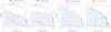 |
Fig. 1. Evolution as a function of the stellar age in million years of the total mass (Mtot, continuous red curve), of the convective core mass (Mcc, continuous blue curve) in solar mass units, of the central ( |


As a result either of mass loss alone (in non-rotating models) or of mass loss and rotationally induced mixing in the outer radiative zone, the surface, and hence the winds, become enriched in 26Al during the core H-burning phase. This surface enrichment lasts until products of core He-burning appear at the surface. From this stage on, the surface abundance of 26Al rapidly decreases, reflecting the destruction of 26Al when interior regions of the star processed by He-burning reactions are exposed at the surface by stellar winds.
Comparing the rotating and the non-rotating model for the 60 M⊙, we see, as was already discussed in Palacios et al. (2005), that rotation favors the 26Al wind enrichment through the following effects:
-
(1)
Species synthesized in the core appear at the surface by rotational mixing on a timescale that is shorter than the time for mass loss to uncover layers whose composition has been changed by nuclear burning. The left panel of Fig. 1 shows that the maximum abundance at the surface is typically reached at an age of ∼3.6 Myr in the non-rotating 60 M⊙ model, while the same surface mass fraction is reached at an age shorter than 2 Myr in the corresponding rotating model.
-
(2)
Due to diffusion of hydrogen from the radiative envelope into the convective core, the convective core remains larger in the rotating model than in the non-rotating model. This also favors a rapid emergence of core H-burning products at the surface.
-
(3)
The core H-burning lifetime is increased by rotation from 3.5 to more than 4.5 Myr in the case of the 60 M⊙ model. This supports 26Al wind ejection during that phase.
We can wonder whether the diffusion of some 25Mg from the radiative envelope into the convective core contributes in some significant way to the increase of 26Al that is produced in the rotating model. We note that the maximum value of the mass fraction of 26Al at the center of the rotating 60 M⊙ is slightly higher than the maximum value reached in the non-rotating corresponding model. This may in part be due to that effect, but it is also due to the difference in the central temperatures between the two models (see the discussion in Sect. 4).
The right panel of Fig. 1 shows the case of a 250 M⊙ very massive star. The following differences with respect to a more classical 60 M⊙ stellar model are evident:
-
(1)
26Al appears significantly earlier at the surface, typically at ages of a few 0.1 Myr. The main reason is that convective cores in very massive stars occupy a much larger fraction of the total mass than they do in less massive stars.
-
(2)
The time difference between reaching the peak abundance at the center and at the surface is reduced. This further reduces the time for the decay of 26Al between these two epochs. This favors larger ejected amounts.
-
(3)
The mass lost with a composition bearing the signatures of H-burning corresponds to 60% of the initial mass for the 250 M⊙ model, while it corresponds to 25% in the case of the rotating 60 M⊙ model and to even less for the non-rotating model. This reflects the increase in mass loss with initial mass. We likely underestimate the mass-loss rates with the present models, and thus their predictions are likely on the conservative side (see the discussion in Sect. 6).
-
(4)
The impact of rotation, while non-negligible, is not as strong in the 250 M⊙ stellar model as in the 60 M⊙ model. This reflects the fact that mass loss by stellar winds and convection dominates the evolution of these stars more strongly than in models with a lower initial mass.
Overall, rotation has a major effect on the increase in the 26Al yields because strong transport from rotational mixing brings large quantities of 26Al to the surface earlier on, enabling the 26Al-enriched envelope to be lost by the winds on longer timescales. While higher initial masses contain a larger reservoir of 25Mg to produce 26Al, they also have stronger mixing due to larger convective cores. This effect, combined with the higher mass loss events, will dominate the rotation effect at very high initial masses.
4. 26Al stellar yields
For each model, we computed the quantity of 26Al that is ejected by stellar winds,  . This quantity was obtained by computing the integral
 (2)
(2)
where τ(M, Z, V) is the lifetime of a star with an initial mass M, an initial metallicity Z, and an initial rotation V.  and Ṁ are the mass fraction of 26Al at the surface and the mass-loss rates for the same model as a function of time. While the decay of 26Al in the stellar interior was accounted for, we did not account for the 26Al decay in the wind ejecta because as explained in the introduction, we need to evaluate the production rate of 26Al.
The stellar yields resulting from our different models can be found in Table A.1 in the appendix and are shown as a function of the initial mass, initial metallicity, and rotation in Fig. 2. The yields become larger than 10−5 M⊙ for initial masses above about 25 M⊙. Above this mass, the 26Al increases in general with the mass, metallicity, and rotation. We can note the following interesting features in Fig. 2:
-
(1)
For initial masses equal to or above 60
 increases with the initial mass and the metallicity according to power laws. For solar metallicity models with rotation, typically
  , and for a rotating 120 M⊙,
  .
. -
(2)
Above 60 M⊙, the differences between rotating and non-rotating models decrease. This reflects the fact that in the very high mass regime, models are more dominated by mass loss and convection than by rotation (at least for the rotational velocities considered here).
-
(3)
Below 60 M⊙, we note that the behavior of the yields as a function of mass can be nonmonotonous (see the non-rotating Z = 0.006 models). At this metallicity, the yield of the 60 M⊙ model typically presents a local maximum. This is due to the specific combination of the effects of stellar winds and convection in this model. At 60 M⊙, this combinatio produces a longer phase than in models with higher initial mass, during which layers processed by H-burning appear at the surface.
-
(4)
The non-rotating models at Z = 0.020 give similar yields as the rotating models at Z = 0.014, showing thus a degeneracy of the yields between increase in rotation and an increase in metallicity.
-
(5)
The rotating models at Z = 0.006 give lower yields than the non-rotating models for masses below about 85 M⊙. This is due to the fact that non-rotating Z = 0.006 models from 40 to 85 M⊙ remain at lower effective temperature than rotating models during He-burning. This induces higher mass losses for these models and results in larger 26Al yields.
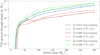 |
Fig. 2. Masses of 26Al ejected by stellar winds during the total stellar lifetime of massive stars with different initial masses, initial metallicities, and rotation rates. |
Figure 3 compares the stellar yields obtained from the present models with and without rotation at Z = 0.014 with models by different authors. The models of Limongi & Chieffi (2018) and Brinkman et al. (2021) displayed here are for single solar metallicity stars. For initial masses above 60 M⊙, the agreement between the predictions of the different models for both rotating and non-rotating models is good in general. In the 30–60 M⊙ mass range, the non-rotating models of this work produce more 26Al than the models of Limongi & Chieffi (2018) and Brinkman et al. (2021), while the rotating models agree. Below 25 M⊙, the present yields are larger than those of Brinkman et al. (2021) and Limongi & Chieffi (2018) because the mass loss in RSG stars is higher, except for the 12–15 M⊙ mass range, where a large difference is displayed by the Limongi & Chieffi (2018) models. This is due to the higher mass-loss rates chosen for these models. They have implemented rates obtained from dust-driven wind during the RSG phase (see Chieffi & Limongi 2013). Except for this mass domain, the models agree well overall. The differences remain at a moderate level, or at least at a level that cannot be distinguished by any current observations.
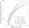 |
Fig. 3. Yields of the present models at Z = 0.014 in comparison to the single-star models of Limongi & Chieffi (2018) and Brinkman et al. (2021). At 50 M⊙, V/Vc = 0.4 is equivalent to 300 km s−1, and at 150 M⊙, it is equivalent to 400 km s−1. |
5. Contribution of the winds of very massive stars to 26Al in the Milky Way
In this section, we compute the quantity of 26Al in the Milky Way that is due to the winds of massive stars. The star formation rate (SFR) is Ψ(R) and is given in terms of the number of stars that forms per unit surface and per unit time at a given galactocentric radius, R, in the Galaxy. We assumed that this function is constant in the past 10 Myr and that the Galaxy is axisymmetric. Our objective here is to estimate the impact of including very massive stars in the 26Al due to stellar winds, rather than to provide a very detailed estimate based on a more complex model for the Galaxy. We normalized the initial mass function, Φ(M)dM, such that
 (3)
(3)
Thus we can interpret Φ(M)dM as the probability that a star of initial mass between M and M + dM is formed when stars with initial masses between 0.07 and 300 M⊙ are formed. We assumed that this function does not vary with time, SFR, or with metallicity, Z. We estimated the production rate of 26Al by stellar winds of stars of a given age t, with an initial mass between M and M + dM, a initial metallicity Z, and initial rotation V at a given galactocentric distance R per unit surface. This quantity is given by  . The contribution of these stars regardless of their age is obtained by integrating this expression over a period that begins at a time t0 − τ(M, Z, V) and t0, thus over a period whose duration is equal to the total lifetime of the star considered. The contribution of stars of a given mass M, regardless of their age, is given by
  . The contribution of stars of different masses is then given by
  , where
 (4)
(4)
is the average mass of 26Al ejected by stellar winds per star formed in a given initial mass interval. The rate of 26Al production in a galactic ring with an internal radius R and width dR is given by  and the total mass in the Galaxy is obtained by integrating the above expression throughout the entire plane of the Milky Way. We call this quantity P26, the galactic production rate. The different rings have different metallicities because the Galaxy presents a metallicity gradient such that the metallicity tends to increase when the galactocentric distance decreases. The above integration needs to account for this, such that the yields that are adopted correspond to the metallicity of each ring, depending on its distance to the galactic center. From this production rate, we can estimate the total amount of 26Al in the Galaxy that is due to stellar winds, M26, assuming that this total amount does not depend on time. As seen in the introduction, it is equal to M26 = P26τ26.
In Fig. 4 we show the result of this integration, adopting the star formation rate from Kubryk et al. (2015)4. We slightly reduced this to obtain a number of core-collapse supernovae of 2 per century in the Milky Way, a Salpeter IMF with α = 2.35, and a metallicity gradient taken from Hayden et al. (2014) (shown in the bottom panel of Fig. 4).
 |
Fig. 4. Milky Way model for 26Al production. Top panel: 26Al production in rings with a width of 0.1 kpc as a function of galactocentric distance. The production is displayed for a Salpeter IMF (α = 2.35) with different maximum masses and with models with and without rotation. The results were obtained taking the SFR and the radial metallicity gradient in the Milky Way into account. The dashed lines show the result when the uncertainties on the metallicity displayed in the bottom panel are considered. The integrated quantities over the whole Milky Way of 26Al are given in the legend. Middle panel: star formation rate as a function of galactocentric distance from Kubryk et al. (2015). Bottom panel: metallicity as a function of galactocentric distance from Hayden et al. (2014). |
The top panel of Fig. 4 shows the 26Al production in rings with a width of 0.1 kpc as a function of galactocentric distance. We considered four different sets of stellar populations, with and without rotation, and including and excluding very massive stars (VMS) in the IMF. These four sets were chosen to underline the effect of rotational mixing on the galactic production of 26Al, and to explore the impact on 26Al production when only a few VMS are included in these populations. The choice of a maximum mass of 300 M⊙ is motivated by the highest initial masses of VMS derived from observations of the Tarantula nebula (Bestenlehner et al. 2020; Brands et al. 2022) in the Large Magellanic Cloud (LMC). The resulting total amount of 26Al produced by these populations ranges from 0.340 M⊙ to 1.431 M⊙. These integrated quantities are displayed in the legend and give the total content of 26Al in the Milky Way that is produced by the winds according to the stellar models. Only stars above 8 M⊙ were used to compute the 26Al lost by the winds. Stars with lower masses have very limited mass loss, and stars with masses lower than 8–12 M⊙ do not even produce 26Al through the Ne–Na and Mg–Al chains because their central temperature during core H-burning5 is lower. The number of stars above 8 M⊙ was computed through the SFR, taking every star in the Milky Way model into account. It is therefore normalized on the whole range from 0.07 M⊙ to the maximum mass included (here either 120 M⊙ or 300 M⊙), as we showed in Eq. (3). The extrapolation into metallicity was made for each initial mass and the yields are compatible with supersolar mass-loss rates.
For every population model, the 26Al peak production is about 4.5 kpc. This is due to the combination of three factors: (1) the peak of the SFR, leading to higher quantities of massive stars, which produce more 26Al; (2) the high metallicity of the inner part of the Milky Way, leading to higher yields, as we showed in Fig. 2, and (3) the surface covered by each bin. While the bins have a width of 0.1 kpc, the surface they cover indeed increases with πR2. The combination of these three components explains the slight shift between the peak of the SFR and the 26Al production. The 26Al production then decreases more abruptly from 6 kpc to the outer parts. This is directly linked to the change in the metallicity trend, which dominates the yields.
The impact of rotation can be seen when the red (non-rotating) and yellow (V/Vc = 0.4) curves are compared. As expected from Sect. 4, the higher yields produced by rotating models lead to a twice higher Galactic 26Al production. The larger effect is seen around the peak of SFR, once again due to the larger number of massive stars, for which all rotating models produce more 26Al at these super solar metallicities.
The impact of including very massive stars can be seen when the red (IMF from 8 to 120 M⊙) and blue (8 to 300 M⊙) curves are compared. The inclusion of the VMS in the stellar population leads to an increase of 120–150% in the 26Al galaxy production. The larger effect is seen once again around the peak of the SFR, where VMS have a higher probability to be produced. This means that a few VMS are sufficient to increase the 26Al production significantly.
Finally, the combined effect of rotation and including the VMS leads to a four times higher 26Al production compared to models that do not account for rotation or VMS. These results show that although very massive stars are very rare (see Sect. 6.2), their effect is still significant because their yields are large. Even a few VMS can have an important impact on the 26Al production at the Galactic scale. This underlines the need to improve our knowledge of their frequency at various metallicities.
6. Discussion and conclusions
6.1. Impact of changing physical ingredients of the models
The evolution of very massive star models mainly depends on the mass-loss rates. We likely underestimate the mass-loss rates here due to the uncertainties on Eddington mass-loss rates (Vink et al. 2011; Bestenlehner et al. 2014; Vink 2018). This means that the 26Al yields might also be underestimated. Increasing the mass-loss rates shortens the period preceding the time when layers that belonged to the convective core appear at the surface, and it increases the quantity of mass that is lost and is enriched in 26Al from that stage on. Fig. 1 and the 250 M⊙ model show that the first effect, that is, shortening the phase before the surface is enriched in 26Al, will have little impact. This phase is already very short. With current mass-loss rates, starting from the time when the surface is enriched in 26Al, more than 100 M⊙ are lost through winds. Increasing the amount of mass that is lost increases the 26Al yield, and will thus increase the contribution of VMS to the global 26Al budget.
The impact of rotational mixing is also very significant, as a population of rotating massive stars produces twice the amount of 26Al as a population of non-rotating stars would in the Milky Way. An increase in rotation rate would result in even higher 26Al yields due to an even stronger transport from rotational mixing, which results in even more 26Al at the surface early on. A less efficient transport of the chemical species will act in the opposite way and would decrease the quantities of 26Al that are ejected by stellar winds. Convection also plays an important role in the transport of 26Al to the surface. With an increase in core size (e.g., as suggested by Martinet et al. 2021; Scott et al. 2021), the transport of 26Al would also be enhanced (as we showed Fig. 1), resulting in higher 26Al yields. We showed that increasing the initial mass increases the mass loss and the convective core size for VMS. This means that increasing the upper mass limit for VMS (e.g., 300–500 M⊙) would also result in an even larger increase of the 26Al galactic production. This is shown in Fig. 5, where the 26Al production in the galaxy is displayed for an IMF with an upper mass limit of up to 500 M⊙. The yields used for stars with initial masses higher than 300 M⊙ were extrapolated and are compatible with the mass loss obtained in the 500 M⊙ models of Yusof et al. (2013). Pushing the upper mass limit to 500 M⊙ increases the total 26Al output from winds by a factor of two in comparison to 300 M⊙ and would account for a very large fraction of galactic 26Al.
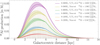 |
Fig. 5. Effect of the upper mass limit on the 26Al production in rings with a width of 0.1 kpc as a function of the galactocentric distance. The same method as in Fig. 4 was used. The 26Al yields above 300 M⊙ are extrapolated. |
Some changes in the nuclear reaction rates may of affect our results. We refer to Iliadis et al. (2011), who reported a detailed study of the dependence of the 26Al masses synthesized by massive stars on the nuclear reaction rates. For the 26Al produced in the H-burning convective core, an important reaction is the one synthesizing 26Al from 25Mg by the 25Mg(p, γ)26Al reaction. A higher reaction rate will increase the quantity of 26Al that is ejected by the winds, and the opposite holds for a lower rate. The median rate by Iliadis et al. (2010) for the 25Mg(p, γ)26Al is 20% lower at most than the rate we used (taken from Iliadis et al. 2001) for the typical temperatures in the H-burning cores of massive stars. This reduction does not have a dramatic impact on the yields. It decreases them slightly if all other parameters remain unchanged. Very recently, the 26Al(n, α) reaction rate has been updated by Lederer-Woods et al. (2021), but this reaction does not impact the phase during which most of the 26Al is produced and ejected. It is therefore not expected to have a strong effect on our results.
6.2. Synthesis of the main results and future perspectives
We computed the yields of 26Al ejected by stellar winds for massive and very massive stars with and without rotation at three different metallicities. We showed that their impact on the global budget of 26Al is significant. This underlines the need to search for such objects and obtain data on their frequency at different metallicities and environments.
Using a simple galactic model to compute the total 26Al mass due to the winds of massive and very massive stars, we obtained that the Galaxy globally contains about 120 000 stars with masses between 8 and 300 M⊙, and 500 stars with initial masses between 120 and 300 M⊙. The variation in these numbers as a function of the galactocentric distance is shown in Fig. 6 (top panel). The lower panel displays the expected number of VMS in a disk around the Sun as a function of the radius of the disk. For example, we expect about 2.5 VMS in a sphere with a radius of 1 kpc around the Sun. These are very rough estimates. Figure 1 in Meynet (1994) gives the maximum distance at which a given mass of 26Al can be detected as a point source by INTEGRAL. When the mass ejected by our rotating model of 180 M⊙ is considered and half of the total yield of 1.3e−03 M⊙ is assumed to still emit γ-ray emission at 1.8 MeV, and when this amount is additionally assumed to be sufficiently concentrated to appear as a point source, then the maximum distance at which such a star would be detectable is 1.25 kpc. This is a very optimistic value. Stochastic effects, the fact that such a source might not appear as point-like or (that the source) presents a smaller amount of nondecayed 26Al than assumed here, would decrease the distance at which the star could be detectable. At the moment, the most convincing candidates for very massive stars have been observed in the LMC (Crowther et al. 2010; Bestenlehner et al. 2020). They are far too far away (roughly 50 kpc) for being observed at 1.8 MeV. An interesting candidate in the Galaxy is Westerhout 49-2 (Wu et al. 2016), which has an estimated mass of 250 M⊙, but lies at 11.1 kpc, still far beyond INTEGRAL sensitivity range. One of the closest candidates would be WR 93 (HD 157504), a 120 M⊙ star (Rate & Crowther 2020). Its distance of 1.76 kpc is beyond the maximum distance at which such a source might be detectable, however. This discussion indicates that while VMS might contribute significantly to the enrichment, this putative contribution is still compatible with the fact that no point-like source of 26Al has been detected so far. While the detection of such a source seems plausible in terms of instrument sensitivity, it would necessitate highly favorable circumstances that seem, for the time being, unlikely.
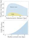 |
Fig. 6. Population of VMS in our Milky Way model. Top panel: number of massive stars (8–120 M⊙) and VMS (120–300 M⊙) in rings with a width of 0.1 kpc as a function of galactocentric distance. We used a Salpeter IMF with α = 2.35 and the SFR from the middle panel of Fig. 4 in Kubryk et al. (2015). Bottom panel: number of VMS in a disk around the Sun as a function of the maximum distance to the Sun, following the same method. |
In addition to the question of the origin of the galactic 26Al, this isotope is also much discussed in two other contexts. There is ample evidence in meteorites for the presence of live 26Al in the cloud that gave birth to the Solar System 4.56 Gyr ago (e.g., Lee et al. 1976; Park et al. 2017). Because of its short half-life, 26Al can help us probe the astrophysical environment of the Solar System at its birth (e.g., Adams & Laughlin 2001). To account for 26Al elevated abundance in the nascent Solar System compared to the 26Al/27Al ratio found in calcium-aluminium-rich inclusions (Jacobsen et al. 2008), in situ irradiation of the protoplanetary disk gas and dust has been proposed (Lee et al. 1977; Gounelle et al. 2001), but is now abandoned after some nuclear cross-sections have been remeasured (Fitoussi et al. 2008). Late delivery by supernovae and AGB stars has long been considered as a possibility to account for Solar System 26Al. Supernovae are now often discarded because they would yield a 60Fe/26Al ratio at least one order of magnitude higher than the ratio that is observed in the early Solar System (Gounelle & Meibom 2008). The probability of associating an AGB star with a star-forming region is very low (Kastner & Myers 1994). The most promising models currently involve the winds of massive stars (Arnould et al. 1997; Gounelle & Meynet 2012). A setting according to which a massive star injects 26Al into a dense shell that it generated itself (Gounelle & Meynet 2012; Dwarkadas et al. 2017) seems to be a likely model (Gounelle 2015).
Another aspect in which 26Al plays an important role is the question of the sources of pristine circumstellar grains, that is, of grains that formed around stars that travel through space and are finally locked in meteorites. Traces of 26Mg due to 26Al that was present at the time of formation of these pristine circumstellar grains, along with the measurements of the abundances of other isotopes, provide a clue about the nature of stars that produce such grains (see, e.g., Zinner et al. 1991; Dauphas & Chaussidon 2011). The proportion in which these grains might be produced around VMS is an interesting open question, as is whether the 26Al that was injected into the protosolar nebula comes from a very massive star.
The critical velocity is the velocity at which the centrifugal force at the equator balances the gravity there. Its expression is taken as indicated by expression (6) in Ekström et al. (2008).
These isotopes are 1H, 3, 4He, 12, 13, 14C, 14, 15N, 16, 17, 18O, 18, 19F, 20, 21, 22Ne, 23Na, 24, 25, 26Mg, 26, 27Al, 28Si, 32S, 36Ar, 40Ca, 44Ti, 48Cr, 52Fe, and 56Ni.
The models at Z = 0.020 were computed with the same equation of state as in Ekström et al. (2012).
To obtain from this SFR, given in solar mass per pc−2 and per billion years (see the middle panel of Fig. 4), an SFR given in number of stars per pc−2 and per billion years, we need to divide by the average mass of a star when stars are formed over the whole mass range between 0.07 and 300 M⊙.
AGB stars can reach a high temperature in their H-burning shell and thus can contribute to the production of this element. However, this is another channel of production that is not discussed here.
Acknowledgments
SM has received support from the SNS project number 200020-205154. GM, SE, CG and DN have received funding from the European Research Council (ERC) under the European Union’s Horizon 2020 research and innovation program (grant agreement No 833925, project STAREX). RH acknowledges support from the World Premier International Research Centre Initiative (WPI Initiative, MEXT, Japan), STFC UK, the European Union’s Horizon 2020 research and innovation program under grant agreement No 101008324 (ChETEC-INFRA) and the IReNA AccelNet Network of Networks, supported by the National Science Foundation under Grant No. OISE-1927130. NY acknowledged the support from Fundamental Research Grant scheme grant number FP042-2021 under Ministry of Higher Education Malaysia. VVD’s work is supported by National Science Foundation award 1911061 to the University of Chicago (PI V. Dwarkadas).
References
- Adams, F. C., & Laughlin, G. 2001, Icarus, 150, 151 [NASA ADS] [CrossRef] [Google Scholar]
- Arnould, M., Paulus, G., & Meynet, G. 1997, A&A, 321, 452 [NASA ADS] [Google Scholar]
- Bennett, M. B., Wrede, C., Chipps, K. A., et al. 2013, Phys. Rev. Lett., 111 [Google Scholar]
- Bestenlehner, J. M., Gräfener, G., Vink, J. S., et al. 2014, A&A, 570, A38 [NASA ADS] [CrossRef] [EDP Sciences] [Google Scholar]
- Bestenlehner, J. M., Crowther, P. A., Caballero-Nieves, S. M., et al. 2020, MNRAS, 499, 1918 [Google Scholar]
- Bouchet, L., Jourdain, E., Roques, J. P., et al. 2003, A&A, 411, L377 [NASA ADS] [CrossRef] [EDP Sciences] [Google Scholar]
- Brands, S. A., de Koter, A., Bestenlehner, J. M., et al. 2022, A&A, 663, A36 [Google Scholar]
- Brinkman, H. E., Doherty, C. L., Pols, O. R., et al. 2019, ApJ, 884, 38 [NASA ADS] [CrossRef] [Google Scholar]
- Brinkman, H. E., den Hartogh, J. W., Doherty, C. L., Pignatari, M., & Lugaro, M. 2021, ApJ, 923, 47 [NASA ADS] [CrossRef] [Google Scholar]
- Caughlan, G. R., & Fowler, W. A. 1988, Atomic Data Nucl. Data Tables, 40, 283 [NASA ADS] [CrossRef] [Google Scholar]
- Cerviño, M., Knödlseder, J., Schaerer, D., von Ballmoos, P., & Meynet, G. 2000, A&A, 363, 970 [NASA ADS] [Google Scholar]
- Champagne, A. E., Brown, B. A., & Sherr, R. 1993, Nucl. Phys. A, 556, 123 [NASA ADS] [CrossRef] [Google Scholar]
- Chen, W., Gehrels, N., & Diehl, R. 1995, ApJ, 440, L57 [NASA ADS] [CrossRef] [Google Scholar]
- Chieffi, A., & Limongi, M. 2013, ApJ, 764, 21 [Google Scholar]
- Crowther, P. A., Schnurr, O., Hirschi, R., et al. 2010, MNRAS, 408, 731 [Google Scholar]
- Dauphas, N., & Chaussidon, M. 2011, Ann. Rev. Earth Planet. Sci., 39, 351 [CrossRef] [Google Scholar]
- de Jager, C., Nieuwenhuijzen, H., & van der Hucht, K. A. 1988, A&AS, 72, 259 [NASA ADS] [Google Scholar]
- del Rio, E., von Ballmoos, P., Bennett, K., et al. 1996, A&A, 315, 237 [NASA ADS] [Google Scholar]
- Diehl, R. 2021, Ap&SS, 366, 104 [NASA ADS] [CrossRef] [Google Scholar]
- Diehl, R., Knödlseder, J., Lichti, G. G., et al. 2003, A&A, 411, L451 [NASA ADS] [CrossRef] [EDP Sciences] [Google Scholar]
- Diehl, R., Halloin, H., Kretschmer, K., et al. 2006, A&A, 449, 1025 [NASA ADS] [CrossRef] [EDP Sciences] [Google Scholar]
- Dwarkadas, V. V., Dauphas, N., Meyer, B., Boyajian, P., & Bojazi, M. 2017, ApJ, 851, 147 [NASA ADS] [CrossRef] [Google Scholar]
- Eggenberger, P., Meynet, G., Maeder, A., et al. 2008, Ap&SS, 316, 43 [Google Scholar]
- Eggenberger, P., Ekström, S., Georgy, C., et al. 2021, A&A, 652, A137 [NASA ADS] [CrossRef] [EDP Sciences] [Google Scholar]
- Ekström, S., Meynet, G., Maeder, A., & Barblan, F. 2008, A&A, 478, 467 [Google Scholar]
- Ekström, S., Georgy, C., Eggenberger, P., et al. 2012, A&A, 537, A146 [Google Scholar]
- Fitoussi, C., Duprat, J., Tatischeff, V., et al. 2008, Phys. Rev. C, 78, 044613 [NASA ADS] [CrossRef] [Google Scholar]
- Georgy, C., Saio, H., & Meynet, G. 2014, MNRAS, 439, L6 [Google Scholar]
- Gounelle, M. 2015, A&A, 582, A26 [NASA ADS] [CrossRef] [EDP Sciences] [Google Scholar]
- Gounelle, M., & Meibom, A. 2008, ApJ, 680, 781 [NASA ADS] [CrossRef] [Google Scholar]
- Gounelle, M., & Meynet, G. 2012, A&A, 545, A4 [NASA ADS] [CrossRef] [EDP Sciences] [Google Scholar]
- Gounelle, M., Shu, F. H., Shang, H., et al. 2001, ApJ, 548, 1051 [NASA ADS] [CrossRef] [Google Scholar]
- Gräfener, G., & Hamann, W. R. 2008, A&A, 482, 945 [Google Scholar]
- Groenewegen, M. A. T. 2012a, A&A, 540, A32 [NASA ADS] [CrossRef] [EDP Sciences] [Google Scholar]
- Groenewegen, M. A. T. 2012b, A&A, 541, C3 [NASA ADS] [CrossRef] [EDP Sciences] [Google Scholar]
- Hayden, M. R., Holtzman, J. A., Bovy, J., et al. 2014, AJ, 147, 116 [NASA ADS] [CrossRef] [Google Scholar]
- Higdon, J. C., Lingenfelter, R. E., & Rothschild, R. E. 2004, ApJ, 611, L29 [NASA ADS] [CrossRef] [Google Scholar]
- Hillebrandt, W., Thielemann, F.-K., & Langer, N. 1987, ApJ, 321, 761 [NASA ADS] [CrossRef] [Google Scholar]
- Iliadis, C., D’Auria, J. M., Starrfield, S., Thompson, W. J., & Wiescher, M. 2001, ApJS, 134, 151 [NASA ADS] [CrossRef] [Google Scholar]
- Iliadis, C., Longland, R., Champagne, A. E., & Coc, A. 2010, Nucl. Phys. A, 841, 323 [NASA ADS] [CrossRef] [Google Scholar]
- Iliadis, C., Champagne, A., Chieffi, A., & Limongi, M. 2011, ApJS, 193, 16 [NASA ADS] [CrossRef] [Google Scholar]
- Jacobsen, B., Yin, Q.-Z., Moynier, F., et al. 2008, Earth Planet. Sci. Lett., 272, 353 [CrossRef] [Google Scholar]
- Kaiser, E. A., Hirschi, R., Arnett, W. D., et al. 2020, MNRAS, 496, 1967 [Google Scholar]
- Kastner, J. H., & Myers, P. C. 1994, ApJ, 421, 605 [NASA ADS] [CrossRef] [Google Scholar]
- Knödlseder, J. 1999, ApJ, 510, 915 [CrossRef] [Google Scholar]
- Knödlseder, J., Bennett, K., Bloemen, H., et al. 1996, A&AS, 120, 327 [NASA ADS] [Google Scholar]
- Knödlseder, J., Bennett, K., Bloemen, H., et al. 1999, A&A, 344, 68 [NASA ADS] [Google Scholar]
- Knödlseder, J., Cerviño, M., Le Duigou, J. M., et al. 2002, A&A, 390, 945 [NASA ADS] [CrossRef] [EDP Sciences] [Google Scholar]
- Krause, M. G. H., Diehl, R., Bagetakos, Y., et al. 2015, A&A, 578, A113 [NASA ADS] [CrossRef] [EDP Sciences] [Google Scholar]
- Krause, M. G. H., Rodgers-Lee, D., Dale, J. E., Diehl, R., & Kobayashi, C. 2021, MNRAS, 501, 210 [Google Scholar]
- Kubryk, M., Prantzos, N., & Athanassoula, E. 2015, A&A, 580, A126 [NASA ADS] [CrossRef] [EDP Sciences] [Google Scholar]
- Lacki, B. C. 2014, MNRAS, 440, 3738 [NASA ADS] [CrossRef] [Google Scholar]
- Lederer-Woods, C., Woods, P. J., Davinson, T., et al. 2021, Phys. Rev. C, 104, L032803 [NASA ADS] [CrossRef] [Google Scholar]
- Lee, T., Papanastassiou, D. A., & Wasserburg, G. J. 1976, Geophys. Rev. Lett., 3, 41 [NASA ADS] [CrossRef] [Google Scholar]
- Lee, T., Papanastassiou, D. A., & Wasserburg, G. J. 1977, ApJ, 211, L107 [NASA ADS] [CrossRef] [Google Scholar]
- Limongi, M., & Chieffi, A. 2006, ApJ, 647, 483 [NASA ADS] [CrossRef] [Google Scholar]
- Limongi, M., & Chieffi, A. 2018, ApJS, 237, 13 [NASA ADS] [CrossRef] [Google Scholar]
- Maeder, A. 1997, A&A, 321, 134 [NASA ADS] [Google Scholar]
- Maeder, A., & Meynet, G. 2000, A&A, 361, 159 [NASA ADS] [Google Scholar]
- Mahoney, W. A., Ling, J. C., Jacobson, A. S., & Lingenfelter, R. E. 1982, ApJ, 262, 742 [NASA ADS] [CrossRef] [Google Scholar]
- Mahoney, W. A., Ling, J. C., Wheaton, W. A., & Jacobson, A. S. 1984, ApJ, 286, 578 [NASA ADS] [CrossRef] [Google Scholar]
- Martinet, S., Meynet, G., Ekström, S., et al. 2021, A&A, 648, A126 [NASA ADS] [CrossRef] [EDP Sciences] [Google Scholar]
- Meyer, B. S., & Clayton, D. D. 2000, Space Sci. Rev., 92, 133 [NASA ADS] [CrossRef] [Google Scholar]
- Meynet, G. 1994, ApJS, 92, 441 [NASA ADS] [CrossRef] [Google Scholar]
- Meynet, G., Arnould, M., Prantzos, N., & Paulus, G. 1997, A&A, 320, 460 [NASA ADS] [Google Scholar]
- Mowlavi, N., & Meynet, G. 2006, New Astron. Rev., 50, 484 [CrossRef] [Google Scholar]
- Mowlavi, N., Knödlseder, J., Meynet, G., et al. 2005, Nucl. Phys. A, 758, 320 [NASA ADS] [CrossRef] [Google Scholar]
- Norris, T. L., Gancarz, A. J., Rokop, D. J., & Thomas, K. W. 1983, Lunar Planet. Sci. Conf. Proc., 88, B331 [Google Scholar]
- Nugis, T., & Lamers, H. J. G. L. M. 2000, A&A, 360, 227 [NASA ADS] [Google Scholar]
- Oberlack, U., Wessolowski, U., Diehl, R., et al. 2000, A&A, 353, 715 [NASA ADS] [Google Scholar]
- Palacios, A., Meynet, G., Vuissoz, C., et al. 2005, A&A, 429, 613 [NASA ADS] [CrossRef] [EDP Sciences] [Google Scholar]
- Park, C., Nagashima, K., Krot, A. N., et al. 2017, Geochim. Cosmochim. Acta., 201, 6 [NASA ADS] [CrossRef] [Google Scholar]
- Pleintinger, M. M. M. 2020, PhD Thesis, Max Planck Institute for Extraterrestrial Physics, Germany [Google Scholar]
- Pleintinger, M. M. M., Siegert, T., Diehl, R., et al. 2019, A&A, 632, A73 [NASA ADS] [CrossRef] [EDP Sciences] [Google Scholar]
- Prantzos, N., & Casse, M. 1986, ApJ, 307, 324 [NASA ADS] [CrossRef] [Google Scholar]
- Rate, G., & Crowther, P. A. 2020, MNRAS, 493, 1512 [NASA ADS] [CrossRef] [Google Scholar]
- Rodgers-Lee, D., Krause, M. G. H., Dale, J., & Diehl, R. 2019, MNRAS, 490, 1894 [NASA ADS] [CrossRef] [Google Scholar]
- Rothschild, R. E., Lingenfelter, R. E., & Higdon, J. C. 2006, New Astron. Rev., 50, 477 [CrossRef] [Google Scholar]
- Scott, L. J. A., Hirschi, R., Georgy, C., et al. 2021, MNRAS, 503, 4208 [NASA ADS] [CrossRef] [Google Scholar]
- Timmes, F. X., & Swesty, F. D. 2000, ApJS, 126, 501 [NASA ADS] [CrossRef] [Google Scholar]
- van Loon, J. T., Cioni, M. R. L., Zijlstra, A. A., & Loup, C. 2005, A&A, 438, 273 [NASA ADS] [CrossRef] [EDP Sciences] [Google Scholar]
- Varendorff, M., & Schoenfelder, V. 1992, ApJ, 395, 158 [NASA ADS] [CrossRef] [Google Scholar]
- Vink, J. S. 2018, A&A, 615, A119 [NASA ADS] [CrossRef] [EDP Sciences] [Google Scholar]
- Vink, J. S., de Koter, A., & Lamers, H. J. G. L. M. 2001, A&A, 369, 574 [NASA ADS] [CrossRef] [EDP Sciences] [Google Scholar]
- Vink, J. S., Muijres, L. E., Anthonisse, B., et al. 2011, A&A, 531, A132 [NASA ADS] [CrossRef] [EDP Sciences] [Google Scholar]
- von Ballmoos, P., Diehl, R., & Schoenfelder, V. 1987, ApJ, 318, 654 [NASA ADS] [CrossRef] [Google Scholar]
- Voss, R., Diehl, R., Hartmann, D. H., et al. 2009, A&A, 504, 531 [NASA ADS] [CrossRef] [EDP Sciences] [Google Scholar]
- Wang, W., Lang, M. G., Diehl, R., et al. 2009, A&A, 496, 713 [NASA ADS] [CrossRef] [EDP Sciences] [Google Scholar]
- Wang, W., Siegert, T., Dai, Z. G., et al. 2020, ApJ, 889, 169 [NASA ADS] [CrossRef] [Google Scholar]
- Wasserburg, G. J., Busso, M., Gallino, R., & Nollett, K. M. 2006, Nucl. Phys. A, 777, 5 [NASA ADS] [CrossRef] [Google Scholar]
- Wu, S.-W., Bik, A., Bestenlehner, J. M., et al. 2016, A&A, 589, A16 [NASA ADS] [CrossRef] [EDP Sciences] [Google Scholar]
- Yanasak, N. E., Wiedenbeck, M. E., Mewaldt, R. A., et al. 2001, ApJ, 563, 768 [NASA ADS] [CrossRef] [Google Scholar]
- Yusof, N., Hirschi, R., Meynet, G., et al. 2013, MNRAS, 433, 1114 [NASA ADS] [CrossRef] [Google Scholar]
- Yusof, N., Hirschi, R., Eggenberger, P., et al. 2022, MNRAS, 511, 2814 [NASA ADS] [CrossRef] [Google Scholar]
- Zahn, J.-P. 1992, A&A, 265, 115 [NASA ADS] [Google Scholar]
- Zinner, E., Amari, S., Anders, E., & Lewis, R. 1991, Nature, 349, 51 [NASA ADS] [CrossRef] [Google Scholar]
Appendix A: Table
Table A.1 presents the stellar 26Al yields from winds obtained in this work as a function of the initial mass and metallicity for non-rotating models and for models that rotate at V/Vc = 0.4.
26Al wind yields (calculated using Eq. 2) in M⊙ units. The VMS models at Z = 0.006 and Z = 0.014 are from Martinet et al. (in prep.) probing initial masses of 180, 250 and 300 M⊙, while the models at Z = 0.020 are from Yusof et al. (2022), with VMS models computed only for 150 and 300 M⊙. More details on the massive stars models at Z = 0.006 can be found in Eggenberger et al. (2021) and in Ekström et al. (2012) for the ones at Z = 0.014. Dashes indicate where the models where not computed.
All Tables
26Al wind yields (calculated using Eq. 2) in M⊙ units. The VMS models at Z = 0.006 and Z = 0.014 are from Martinet et al. (in prep.) probing initial masses of 180, 250 and 300 M⊙, while the models at Z = 0.020 are from Yusof et al. (2022), with VMS models computed only for 150 and 300 M⊙. More details on the massive stars models at Z = 0.006 can be found in Eggenberger et al. (2021) and in Ekström et al. (2012) for the ones at Z = 0.014. Dashes indicate where the models where not computed.
All Figures
|
Fig. 1. Evolution as a function of the stellar age in million years of the total mass (Mtot, continuous red curve), of the convective core mass (Mcc, continuous blue curve) in solar mass units, of the central ( |
| In the text | |
|
Fig. 2. Masses of 26Al ejected by stellar winds during the total stellar lifetime of massive stars with different initial masses, initial metallicities, and rotation rates. |
| In the text | |
|
Fig. 3. Yields of the present models at Z = 0.014 in comparison to the single-star models of Limongi & Chieffi (2018) and Brinkman et al. (2021). At 50 M⊙, V/Vc = 0.4 is equivalent to 300 km s−1, and at 150 M⊙, it is equivalent to 400 km s−1. |
| In the text | |
|
Fig. 4. Milky Way model for 26Al production. Top panel: 26Al production in rings with a width of 0.1 kpc as a function of galactocentric distance. The production is displayed for a Salpeter IMF (α = 2.35) with different maximum masses and with models with and without rotation. The results were obtained taking the SFR and the radial metallicity gradient in the Milky Way into account. The dashed lines show the result when the uncertainties on the metallicity displayed in the bottom panel are considered. The integrated quantities over the whole Milky Way of 26Al are given in the legend. Middle panel: star formation rate as a function of galactocentric distance from Kubryk et al. (2015). Bottom panel: metallicity as a function of galactocentric distance from Hayden et al. (2014). |
| In the text | |
|
Fig. 5. Effect of the upper mass limit on the 26Al production in rings with a width of 0.1 kpc as a function of the galactocentric distance. The same method as in Fig. 4 was used. The 26Al yields above 300 M⊙ are extrapolated. |
| In the text | |
|
Fig. 6. Population of VMS in our Milky Way model. Top panel: number of massive stars (8–120 M⊙) and VMS (120–300 M⊙) in rings with a width of 0.1 kpc as a function of galactocentric distance. We used a Salpeter IMF with α = 2.35 and the SFR from the middle panel of Fig. 4 in Kubryk et al. (2015). Bottom panel: number of VMS in a disk around the Sun as a function of the maximum distance to the Sun, following the same method. |
| In the text | |
Current usage metrics show cumulative count of Article Views (full-text article views including HTML views, PDF and ePub downloads, according to the available data) and Abstracts Views on Vision4Press platform.
Data correspond to usage on the plateform after 2015. The current usage metrics is available 48-96 hours after online publication and is updated daily on week days.
Initial download of the metrics may take a while.