| Issue |
A&A
Volume 663, July 2022
|
|
|---|---|---|
| Article Number | A100 | |
| Number of page(s) | 13 | |
| Section | Planets and planetary systems | |
| DOI | https://doi.org/10.1051/0004-6361/202243490 | |
| Published online | 19 July 2022 | |
Precision measurement of a brown dwarf mass in a binary system in the microlensing event
OGLE-2019-BLG-0033/MOA-2019-BLG-035★
1
Dipartimento di Fisica e Astronomia “Galileo Galilei”, Università di Padova,
Vicolo dell’Osservatorio 3,
Padova
35122, Italy
2
Observatory, University of Warsaw,
Al. Ujazdowskie 4,
00-478
Warszawa, Poland
3
Dipartimento di Fisica “E.R. Caianiello”, Università degli studi di Salerno,
Via Giovanni Paolo II 132,
84084
Fisciano (SA), Italy
e-mail: valboz@sa.infn.it
4
Istituto Nazionale di Fisica Nucleare, Sezione di Napoli,
Via Cintia,
80126
Napoli (NA), Italy
5
School of Mathematical and Computational Sciences, Massey University,
Auckland
0745, New Zealand
6
Center for Astrophysics, Harvard & Smithsonian,
60 Garden St.,
Cambridge, MA
02138, USA
7
Department of Physics, Isfahan University of Technology,
Isfahan, Iran
8
Department of Physics, University of Warwick,
Gibbet Hill Road,
Coventry
CV4 7AL, UK
9
Institute for Space-Earth Environmental Research, Nagoya University,
Nagoya
464-8601, Japan
10
Code 667,
NASA Goddard Space Flight Center,
Greenbelt, MD
20771, USA
11
Department of Astronomy, University of Maryland,
College Park, MD
20742, USA
12
Department of Earth and Planetary Science, Graduate School of Science, The University of Tokyo,
7-3-1 Hongo, Bunkyo-ku,
Tokyo
113-0033, Japan
13
Instituto de Astrofísica de Canarias,
Vía Láctea s/n,
38205
La Laguna, Tenerife, Spain
14
Department of Earth and Space Science, Graduate School of Science, Osaka University,
Toyonaka, Osaka
560-0043, Japan
15
Zentrum für Astronomie der Universität Heidelberg, Astronomisches Rechen-Institut,
Mönchhofstr. 12–14,
69120
Heidelberg, Germany
16
Department of Physics, University of Auckland,
Private Bag 92019,
Auckland, New Zealand
17
Department of Physics, The Catholic University of America,
Washington, DC
20064, USA
18
University of Canterbury Mt. John Observatory,
PO Box 56,
Lake Tekapo
8770, New Zealand
19
IPAC,
Mail Code 100-22, Caltech, 1200 E. California Blvd.,
Pasadena, CA
91125, USA
20
Jet Propulsion Laboratory, California Institute of Technology,
4800 Oak Grove Drive,
Pasadena, CA
91109, USA
21
Department of Astronomy, Ohio State University,
140 W. 18th Ave.,
Columbus, OH
43210, USA
22
Max-Planck-Institute for Astronomy,
Königstuhl 17,
69117
Heidelberg, Germany
23
Department of Particle Physics and Astrophysics, Weizmann Institute of Science,
Rehovot
76100, Israel
24
Department of Astronomy, Tsinghua University,
Beijing
100084, PR China
25
Centre for Exoplanet Science, SUPA, School of Physics & Astronomy, University of St Andrews,
North Haugh,
St Andrews
KY16 9SS, UK
26
Centre for ExoLife Sciences, Niels Bohr Institute,
Øster Voldgade 5,
1350
Copenhagen, Denmark
27
Unidad de Astronomía, Universidad de Antofagasta,
Av. Angamos 601,
Antofagasta, Chile
28
Centre for Electronic Imaging, Department of Physical Sciences, The Open University,
Milton Keynes
MK7 6AA, UK
29
Instituto de Astronomía y Ciencias Planetarias, Universidad de Atacama,
Avenida Copayapu 485,
Copiapó, Atacama, Chile
30
Universität Hamburg, Faculty of Mathematics, Informatics and Natural Sciences, Department of Earth Sciences, Meteorological Institute,
Bundesstrasse 55,
20146
Hamburg, Germany
31
Instituto de Astrofísica Pontificia Universidad Católica de Chile,
Avenida Vicuna Mackenna 4860,
Macul, Santiago, Chile
32
Department of Physics, Sharif University of Technology,
PO Box 11155-9161
Tehran, Iran
33
Institute for Astronomy, University of Edinburgh, Royal Observatory,
Edinburgh
EH9 3HJ, UK
34
Astrophysics Group, Keele University,
Staffordshire
ST5 5BG, UK
35
National Astronomical Observatories, Chinese Academy of Sciences,
Beijing
100101, PR China
36
Las Cumbres Observatory,
6740 Cortona Drive, suite 102,
Goleta, CA
93117, USA
37
School of Physics and Astronomy, Tel-Aviv University,
Tel-Aviv
6997801, Israel
38
Auckland Observatory,
Auckland, New Zealand
39
Kumeu Observatory,
Kumeu, New Zealand
40
Universidade Federal do Rio Grande do Norte (UFRN), Departamento de Fśica,
59078-970
Natal, RN, Brazil
41
Laboratório Nacional de Astrofísica,
Rua Estados Unidos 154,
37504-364
Itajubá - MG, Brazil
42
Department of Physics, Chungbuk National University,
Cheongju
28644, Republic of Korea
43
Farm Cove Observatory, Centre for Backyard Astrophysics,
Pakuranga, Auckland, New Zealand
44
Klein Karoo Observatory, Centre for Backyard Astrophysics,
Calitzdorp, South Africa
45
Institute for Radio Astronomy and Space Research (IRASR), AUT University,
Auckland, New Zealand
Received:
7
March
2022
Accepted:
3
April
2022
Context. Brown dwarfs are transition objects between stars and planets that are still poorly understood, for which several competing mechanisms have been proposed to describe their formation. Mass measurements are generally difficult to carry out for isolated objects as well as for brown dwarfs orbiting low-mass stars, which are often too faint for a spectroscopic follow-up.
Aims. Microlensing provides an alternative tool for the discovery and investigation of such faint systems. Here, we present an analysis of the microlensing event OGLE-2019-BLG-0033/MOA-2019-BLG-035, which is caused by a binary system composed of a brown dwarf orbiting a red dwarf.
Methods. Thanks to extensive ground observations and the availability of space observations from Spitzer, it has been possible to obtain accurate estimates of all microlensing parameters, including the parallax, source radius, and orbital motion of the binary lens.
Results. Following an accurate modeling process, we found that the lens is composed of a red dwarf with a mass of M1 = 0.149 ± 0.010 M⊙ and a brown dwarf with a mass of M2 = 0.0463 ± 0.0031 M⊙ at a projected separation of a⊥ = 0.585 au. The system has a peculiar velocity that is typical of old metal-poor populations in the thick disk. A percent-level precision in the mass measurement of brown dwarfs has been achieved only in a few microlensing events up to now, but will likely become more common in the future thanks to the Roman space telescope.
Key words: gravitational lensing: micro / binaries: general / brown dwarfs / stars: low-mass
The lightcurves are only available at the CDS via anonymous ftp to cdsarc.u-strasbg.fr (130.79.128.5) or via http://cdsarc.u-strasbg.fr/viz-bin/cat/J/A+A/663/A100
© ESO 2022
1 Introduction
The low-mass end of main-sequence stars is conventionally set by the minimum mass needed to trigger hydrogen burning in the core. This corresponds to 0.078 M⊙ at solar metallicity (Auddy et al. 2016). Objects below this mass, classified as brown dwarfs (BDs), may still burn deuterium for a short phase and then cool down, similarly to the case of planets (Burrows et al. 1997). The distinction between planets and BDs is more vague because the deuterium-burning limit of 0.013⊙ (Spiegel et al. 2011) has little impact on the global properties and evolution of these substellar objects. It is also known that the formation of BDs may occur via the instability and collapse of gas clouds with the same Jeans mechanism that generates stars (Béjar et al. 2001). However, this mechanism rapidly becomes inefficient at low masses and may not fully account for the number of observed BDs (Larson 1992; Elmegreen 1997). On the other hand, bigger planets formed by core accretion may exceed the above-mentioned planet-BD threshold and be classified as BDs, although they are, in fact, formed starting from a rock-ice core (Mollière & Mordasini 2012; Whitworth et al. 2007). However, the lack of transiting BDs in Kepler discoveries and of BD companions to Sun-like stars hints at some migration or instability mechanism depleting planetary systems of overly massive objects (Marcy & Butler 2000; Grether & Lineweaver 2006; Johnson et al. 2011). Following a different route, lower-mass stars may be naturally formed in binaries or multiples via the turbulent fragmentation of the pro-tostellar clouds, with some of the low-mass companions lying in the BD mass range (Padoan et al. 2005).
Confronting the efficiency of the alternative channels for the formation of BDs is difficult because these elusive objects are intrinsically dim and can only be detected when they are relatively young and hot (Close et al. 2007; Lafrenière et al. 2007). Space-borne instruments are well suited for the detection of young BDs in the infrared (Spezzi et al. 2011; McLean et al. 2003), with a recent direct radio discovery of a BD having been reported by Vedantham et al. (2020). Similar complications exist for small companions to red dwarfs as well, as red dwarfs are typically too faint to act as appropriate targets for spectroscopic follow-up (Sahlmann et al. 2011). Thus, the mass and the nature of such companions remain poorly known.
The low luminosity of brown and red dwarfs is not a limitation if observations rely on the light of some other sources, as in gravitational microlensing. Indeed, most of the lenses populating our Galaxy and causing the magnification of background sources are believed to be low-mass stars or possibly BDs and even rogue planets (Mróz et al. 2017, 2019 Mróz et al. 2020; Kim et al. 2021; Ryu et al. 2021). Therefore, microlensing provides a key to explore the low end of the mass function throughout our Galaxy (Koshimoto et al. 2021). However, the mass measurement of individual lenses is generally difficult because the information stored in a basic microlensing event is very degenerate. Subtle anomalies, higher order effects, or additional observations are needed to resolve such degeneracies. Fortunately, this happens routinely for a sizeable fraction of microlensing events, leading to relatively good mass estimates of otherwise unde-tectable objects based on a variety of methods (An et al. 2002; Wyrzykowski & Mandel 2020).
Concerning the discoveries of BDs with microlensing, the first isolated brown dwarf was recognized in the microlensing event OGLE-2007-BLG-224 (Gould et al. 2009). Often, BDs as companions to stellar primaries have been previously discovered (Bozza et al. 2012; Ranc et al. 2015). Interestingly, several binary systems composed of BDs have been detected (Choi et al. 2013), as well as a case of a planet orbiting a BD just slightly below the hydrogen-burning limit (Bennett et al. 2008). The growing number of BD discoveries allows for microlensing to confirm previous considerations about the existence of a BD desert at short periods around Sun-like stars, with some possible accumulation at intermediate periods (Ranc et al. 2015). Of particular note are those discoveries with very precise mass measurements, with a better than 10% accuracy having been reached in a number of instances (Gould et al. 2009; Choi et al. 2013; Han et al. 2013; Ranc et al. 2015; Albrow et al. 2018).
In this paper, we report our analysis of OGLE-2019-BLG-0033/MOA-2019-BLG-035, a long timescale event that has been well covered by many ground telescopes, including surveys and follow-ups, allowing for a very good determination of parallax and finite-source effects. With the help of Spitzer data from space, the best model for this binary lens event including orbital motion can be uniquely determined. With all this information, it is possible to achieve exceptional precision in the mass measurement of the two components of the system, which have turned out to be a red and brown dwarf at an intermediate separation.
In Sect. 2, we present the observations used for the analysis. In Sect. 3, we describe the modeling stages of the microlensing light curve. In Sect. 4, we deal with the source analysis using the color-magnitude diagram from the MOA telescope. In Sect. 5, we finalize the full interpretation of the model presenting the physical parameters. Section 6 contains a discussion on precise mass measurements by microlensing and their contribution to the understanding of BDs. We conclude with a brief summary in Sect. 7.
2 Observations
The microlensing event OGLE-2019-BLG-0033/MOA-2019-BLG-035 was announced by the OGLE collaboration at the beginning of the 2019 bulge season on February 19 and independently found by MOA four days later. Its equatorial coordinates (J2000.0) are RA= 18 : 08 : 38.26, Dec= −30 : 03 : 38.7, corresponding to Galactic coordinates l = 1.53°, b = −4.90°. Figure 1 shows all observations taken on OGLE-20 9-BLG-0033 by different ground telescopes and from Spitzer. We summarize these observations and their reduction in this section.
The OGLE observations were carried out with the 1.3-m Warsaw telescope located at the Las Campanas Observatory, Chile. It was equipped with a 32-CCD mosaic camera covering 1.4 square degrees on the sky with a pixel scale of 0.26 arcsec per pixel. Most observations were obtained through the I-band filter (exposure time of 100 sec) for time series with occasional observations in the V–band for color information. The lens is located in the BLG521 OGLE field which was observed with an average cadence of less than one observation per night. Photometry of OGLE-2019-BLG-0033 was derived using the standard OGLE photometric pipeline (Udalski et al. 2015), based on difference image analysis implementation by Wozniak (2000).
The MOA collaboration is carrying out a high cadence microlensing survey with a 1.8-m MOA-II telescope at Mt. John University Observatory in New Zealand (Bond et al. 2001; Sumi et al. 2003). The telescope has a 2.2 deg2 FOV, with a 10-chip CCD camera. The main observations are taken using the MOA-Red filter, which corresponds to the standard Cousins R- and I-bands (630–1000nm). The MOA images were reduced with MOA’s implementation (Bond et al. 2001) of the difference image analysis (DIA) method (Tomaney & Crotts 1996; Alard & Lupton 1998; Alard 2000). In the MOA photometry, we de-trend the systematic errors that correlate with the seeing and airmass, as well as the motion (due to differential refraction) of a nearby, possibly unresolved star (Bond et al. 2017).
OGLE-2019-BLG-0033 was selected for Spitzer observations on 2019 May 10 at UT 04:11 (HJD′ = HJD-2400000 = 8613.67), well before the binary anomaly was identified. It was selected as a “subjective, immediate” target with an “objective” cadence following the protocols described by Yee et al. (2015). This cadence resulted in roughly one observation per day starting in Week 2 of the 2019 Spitzer campaign (the first week the target was observable). The Spitzer observations were taken using the 3.6 μm (L-band) channel of the IRAC camera. Each observation consisted of six dithered exposures. Because the target was very bright, the first ten epochs were taken with 12s exposures. Then, 30s exposures were used after HJD′ = 8692, once it was established that the target would not be saturated as seen from Spitzer. The Spitzer data were reduced using the photometry pipeline developed by Calchi Novati et al. (2015) for IRAC data in crowded fields. Because OGLE-2019-BLG-0033 was a Spitzer target outside of the KMTNet fields (Kim et al. 2016) and the OGLE cadence was < 1 obs per night, follow-up telescopes have been particularly useful.
The Microlensing Follow-Up Network (μFUN) observed this event in the I- and H-bands using the SMARTS Cerro Tololo 1.3m telescope (CT13) in Chile. Initially, these observations were taken primarily in order to measure the (I – H) color of the source. However, starting from HJD′ = 8666, this event was added to a group of events followed at a higher cadence in order to increase the sensitivity to small planets. Hence, OGLE-2019-BLG-0033 received a couple of observations per night from CT13 as time allowed. On 2019 July 19, μFUN recognized that the event was deviating from a point lens and sent out an anomaly alert at UT 17:09. As a result, additional follow-up observations were taken by several μFUN observatories, including the Auckland Observatory (AO), Farm Cove Observatory (FCO), and Kumeu Observatory in New Zealand: AO and Kumeu observed using a Wratten #12 filter (designated R), while FCO observed without a filter (designated U for “unfiltered”). Observations were also obtained in the i band by the 1.6m telescope at Observatorio do Pico dos Dias (OPD) located in Brazil and using a clear filter (also designated U) from Klein Karoo Observatory in South Africa. All μFUN data, including CT13, were reduced using the DoPHOT pipeline (Schechter et al. 1993).
The Las Cumbres Observatory (LCO) global network conducted observations using the 0.4 m telescope at the South African Astronomical Observatory (SAAO) in South Africa and the Haleakala Observatory in Hawaii (FTN). The LCO data were reduced using a custom DIA pipeline (Zang et al. 2018) based on the ISIS package (Alard & Lupton 1998; Alard 2000).
The MiNDSTEp data were obtained using the Danish 1.54m Telescope at ESO La Silla Observatory in Chile, as part of the MiNDSTEp microlensing follow-up program (Dominik et al. 2010). The Danish 1.54m Telescope is equipped with a multiband EMCCD instrument (Skottfelt et al. 2015) providing shifted and co-added images in its custom red and visual passbands. This work utilizes red band time-series photometry which was reduced with a modified version of DANDIA (Bramich 2008; Bramich et al. 2013). In total, 817 observations were taken, of which 3 were discarded based on photometric scale factors close to zero, which serves as proxy for identifying system-atics in photometric measurements (most commonly overcast skies).
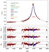 |
Fig. 1 Light curve of the event OGLE-2019-BLG-0033 showing all observations from different telescopes as described in the text. The black curve is the best microlens-ing model for ground observers, and the red curve is the best model for Spitzer observations, as described in Sect. 3. In the bottom panel, we show the residuals from several models: best model including the parallax and orbital motion, best model with parallax without orbital motion, and best static model without parallax. |
3 Modeling
Microlensing occurs when the lens passes close to the line of sight to a background source whose flux is thus temporarily magnified. The fundamental angular scale that governs microlensing is the angular Einstein radius:
 (1)
(1)
where M is the total lens mass, κ = 4G/(c2au) combines Newton’s constant, the speed of light, and the astronomical unit, and where
 (2)
(2)
is the difference of the lens and source parallaxes.
For a lens moving with respect to the source with proper motion μ, the timescale of the event (or Einstein time) is
 (3)
(3)
The magnification of the source is maximum at the time of closest approach of the lens to the source line of sight, t0, when the minimum angular separation, u0, is reached (expressed in units of the Einstein radius).
If the lens is composed of two masses, besides tE, t0, and u0, the light curve also depends on additional parameters: the mass ratio, q, the projected angular separation in Einstein radii, s, the position angle α of the second mass relative to the primary measured from the lens proper motion vector, and the source angular radius, ρ*, in units of the Einstein radius.
For long-timescale microlensing events, the motion of the Earth around the Sun must be taken into account, as it affects the apparent relative proper motion of lens and source. Such an annual parallax effect is modeled by two additional parameters, πE,N and πE,E, representing the northern and eastern components of the parallax vector, whose modulus is
 (4)
(4)
and whose direction is given by the lens-source proper motion direction (Gould 1992, Gould 2000). A binary lens model including parallax, thus, is characterized by nine parameters.
Finally, as the two lenses are gravitationally bound, they should orbit around their common center of mass. The full Keplerian motion can be modeled by five additional parameters (Skowron et al. 2011). However, because the duration of the microlensing event is often too short to derive a full orbit, it is generally sufficient to add a minimal set of three velocity components to obtain a circular orbit (Skowron et al. 2011; Bozza et al. 2021). A two-component orbital motion, sometimes used for minimal fits, should be avoided as it leads to unphysical orbital trajectories (Bozza et al. 2021; Ma & Zhu 2021). The three components of the velocity are  , where sz is the separation between the two lenses along the line of sight in Einstein radii. A binary lens model including parallax and orbital motion has, thus, 12 parameters.
As the lens moves in front of the source (or, equivalently, the source moves behind the lens), the source may enter regions in which new images are created. The boundaries of such regions are called caustics and determine the overall shape of the light curve for binary lenses.
Figure 2 provides a zoom-in on the double-peak region of the light curve of OGLE-2019-BLG-0033, occurring at moderate magnification (Amax ≃ 15). This structure indicates that the central caustic generated by the lens has a typical astroid shape, which may arise either for close binary lenses or for a lens perturbed by a wide companion (Dominik 1999; Bozza 2000). Figure 3 shows this shape as reconstructed by the best models to be described in this section, with a zoom-in shown in Fig. 4.
The presence of a double-peak was immediately recognized during the observation campaigns, as noted in Sect. 2. Automatic modeling of the available online photometry by RTModel1 found a full solution on 2019 August 25, including annual parallax and finite source effect, with the conclusion that the system was made up of a red and brown dwarf, with masses very similar to those reported following the full analysis.
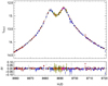 |
Fig. 2 Zoom on the double-peak region of the light curve. The color-coding for the observations is the same as in Fig. 1. |
3.1 Detailed Modeling Procedure
The photometry collected by all observatories has been reduced according to the procedures described in Sect. 2. We noted that the Spitzer light curve consists of 29 data points spanning 32 nights. These observations are around the peak of the magnification as seen from the ground observations and are very far from the baseline. Without a baseline, Spitzer observations for this event must be complemented by a flux constraint to be included in the analysis (Calchi Novati et al. 2015). Given the special role of the Spitzer data, which provide an independent determination of the parallax with respect to ground data, we decided to first analyze the ground data alone and obtain a first determination of all microlensing parameters of the event. As a second step, using the flux constraint on Spitzer data and comparing with the measured flux, we infer the geometry of the event as seen from the satellite alone. From this we obtain an independent estimate of the parallax that can be compared with the ground-only measurement to provide an important confirmation of the previous result (Gould & Yee 2012). Finally, we present the results for a combined fit of ground + Spitzer data and we discuss the impact of satellite data in the fit.
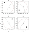 |
Fig. 3 Caustics of the four binary lens models examined in our analysis, with the best model labeled as A. The source trajectories are also shown as seen from Earth observatories (black) and from Spitzer (red). |
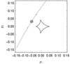 |
Fig. 4 Zoom-in on the caustic of the best binary lens model with the source trajectory. The size of the source is shown by the gray disk. |
3.1.1 Modeling of Ground Data
With all the available ground data, we re-ran an RTModel search and evaluated all possible competing models. This first run confirmed the results of the preliminary model. However, it is widely known that parallax measurements using satellites are subject to a four-fold satellite degeneracy (Refsdal 1966; Gould 1994a), which corresponds to four competing models that can be obtained by reflection of the source trajectory around the binary-lens axis and by changes of signs in the parallax components. These four models are labeled A, B, C, and D (as shown in Fig. 3). We then decided to check all possibilities in parallel before dismissing any of them. Moreover, for all the models, we obtained a significant improvement by including orbital motion. It is important to correctly account for this last additional effect because it impacts the estimated components of the parallax (Skowron et al. 2011; Batista et al. 2011). We work in the geocentric frame, setting the reference time for the parallax and orbital motion calculations as t0,orb = t0,par = t0.
After this first step, we go on to re-normalize the error bars of all datasets to ensure that χ2/d.o.f. = 1 for the model with the lowest χ2. This standard procedure makes the fit more robust against possible low-level unknown systematics in the data (Miyake et al. 2011). However, we note that all datasets very accurately follow the best model with no particular deviations, as is evident from Figs. 1–2.
With the re-normalized uncertainties and including appropriate limb darkening coefficients for the source in each band (as detailed in Sect. 4), we ran a Markov chain Monte Carlo with one million samples to explore the parameter space around each model. As for RTModel, the microlensing magnification has been computed by the contour integration code VBBinaryLensing2 (Bozza 2010; Bozza et al. 2018, Bozza et al. 2021). The final parameters for each of the four models are listed in Table 1, where we see that the model labeled A stands out with a Δχ2 = 120 from the closest alternative, which is B. In this table we also include the baseline magnitude for OGLE (IOGLE) and the relative blending fraction BFOGLE, namely, the ratio of the contaminating flux from unresolved stars in the blend to the source flux.
For reference, the best model without orbital motion has Δχ2 = +477 with respect to the best solution. The static model without parallax has Δχ2 = +4020. The best binary source model with a single-lens has Δχ2 = +906, while a model with a binary lens including parallax and xallarap (i.e., a source moving around an unseen companion) gives Δχ2 = +215.
The quality of the ground data and coverage of the light curve, combined with the favorable case of a giant source with negligible blending and a long timescale (tE ≃ 103.6 days), allow us to obtain particularly accurate estimates for all the microlens-ing parameters. The event can be clearly ascribed to a close binary system with a secondary object that is one-third as massive as the primary. The source size parameter, ρ*, is measured at 3% precision, in spite of the fact that the source trajectory does not cross any caustics. This is due to the fact that the giant source passes over the magnified lobes surrounding two cusps of the astroid caustic. Its size is large enough to make it sensitive to the steep gradients in these regions, as shown in Fig. 4. Both parallax components are also particularly accurate even when using ground data alone without any continuous or discrete degeneracies (Refsdal 1966; Gould 1994b; Smith et al. 2003; Poindexter et al. 2005). Finally, orbital motion is clearly measured in its first component: ds/dt, it is marginally seen in: dα/dt, while only an upper limit can be given to the radial velocity component. The blending ratio is close to zero, with the flux vastly dominated by the magnified giant source, which makes the source analysis easier.
Parameters of the best microlensing models found with ground-only data.
3.1.2 Parallax Determination from Spitzer
In principle, the parallax determination from the ground can be affected by competing higher order effects, such as the orbital motion of the lens, xallarap, or even long-term source variability. Thus, an independent confirmation of the result using a different observation point is desirable. The existence of Spitzer data provides the opportunity to carry out such a test and check the consistency of the results. In order to do this, we followed the cheap space-based parallax method suggested by Gould & Yee (2012) and tested previously by Shin et al. (2018, 2022).
The ground model confirms that the blending in OGLE photometry, if any, is negligible. However, Spitzer has a pixel scale of 1.2″ compared to 0.26″ for OGLE, therefore being more exposed to blending by nearby objects. Fortunately, no stars within this angular distance appear in OGLE images or in OGLE catalog and, indeed, the source appears well isolated in the Spitzer images. As a further proof that the source does not suffer from contamination in Spitzer images, we compare the color-magnitude-diagram (CMD) obtained using MOA observations in V and R bands (top panel of Fig. 5) with a CMD obtained using OGLE I-band and Spitzer L-band (bottom panel of Fig. 5). In both cases, the source lies just slightly below the centroid of the red clump, demonstrating that the ground and space measurements refer to the same object with no appreciable blending.
Following the strategy outlined by Yee et al. (2013) and based upon Spitzer photometry of field stars cross-matched with OGLE-EWS CMD, we evaluate a corresponding color, I − L = −5.67 ± 0.06, for a zero point at 25 for Spitzer. With an OGLE baseline of I = 15.65, this translates to the following baseline flux for Spitzer:
 (5)
(5)
in instrumental units.
On the other hand, the Spitzer measurements during the observation window show a quite flat light curve. In particular, at time t0, the two closest observations average at  . This means that the magnification as seen from Spitzer at this time is
 (6)
(6)
where again we are assuming that blending is negligible, as indicated by the ground-data model.
If the lens were a point mass, we would simply invert the Paczynski formula:
 (7)
(7)
to obtain the angular separation of source and lens in Einstein radii
![$u\left( A \right) = \sqrt {2[{{(1 - {A^{ - 2}})}^{ - 1/2}} - 1]}.$](/articles/aa/full_html/2022/07/aa43490-22/aa43490-22-eq57.png) (8)
(8)
The derived separation obtained thus is |u0,Sp|=0.460 ± 0.015. Since our lens is binary, we can make a more detailed search for angular separations yielding a magnification equal to A0,Sp. We find that 0.44 < |u0,Sp| < 0.48 depending on the orientation of the source as seen from Spitzer with respect to the binary lens axis. This is very similar to the result for a single lens quoted before. Indeed, the Spitzer separation is seven times larger than the size of the caustic in Einstein units, so that perturbations of the magnification from lens binarity are small.
The offset of the source as seen from Spitzer with respect to the ground again depends on the unknown relative position angle. Therefore, this offset may range from |u0,Sp| − |u0| to |u0,Sp| + |u0|. Combining the uncertainties, we set Δu0 = |u0,Sp| − u0| = 0.46 ± 0.07.
At time t0, the separation of Spitzer from Earth projected orthogonally to the line of sight was d0,Sp = 1.51 au. Thus, we finally obtain:
 (9)
(9)
This can be compared to the result from the ground-only fit, which corresponds to:
 (10)
(10)
We stress that the only information from the ground model used in the derivation of the Spitzer parallax was the time of the peak, t0, the source separation from the lens, u0, and the absence of blending; thus, with regard to the parallax, the two results can be considered completely independent of each other. The consistency becomes even more evident when we note that for the best model A, the predicted offset of the source δu as seen from Spitzer is indeed close the maximal value quoted before. We conclude that Spitzer fully validates the ground-only derived parallax making our result more robust against any possible sources of systematics that would remain uncontrolled with ground-only data.
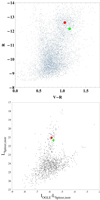 |
Fig. 5 Color-magnitude diagrams using different resources. Top panel: CMD of stars in the 2′ field of the event OGLE-2019-BLG-0033 built from MOA observations. The red dot corresponds to the center of the red clump and the green dot shows the position of the source. Bottom panel: CMD built from I-band observations from OGLE and L-band measurements from Spitzer. |
3.1.3 Models Including Ground and Spitzer Data
As a final check for the consistency between ground and Spitzer observations, we conducted Markov chain explorations of the parameter space including Spitzer data for all four configurations studied in Sect. 3.1.1. In these fits, we forced the Spitzer flux to fulfill the constraint (5) so as to keep the exploration within physically acceptable regions. The results are summarized in Table 2, where we see that model A is largely preferred also by Spitzer data, with a Δχ2 = 46, compared to Δχ2 > 71 for other models. The value of the parallax parameter πE remains within 2σ for model A, while it is significantly altered in other models, proving that the space parallax would be in tension with the ground parallax in these cases. This tension is apparent in the light curves of these models, which predict a declining trend for the Spitzer light curve that is not observed. The Spitzer light curve is quite flat in the observation window, as correctly predicted by model A as shown in Fig. 1. Therefore, Spitzer provides an additional strong confirmation of the model found using ground data only. In Fig. 6, we can appreciate how accurate the parallax measurement is for our event and the consistency of the fits performed with or without Spitzer data in model A.
Taken the other way round, the full consistency of ground and Spitzer parallaxes also demonstrates that in this case Spitzer photometry was free of any important systematic effects, which may be present when the source is faint or blended (Koshimoto & Bennett 2020) and that a correct use of the color constraint makes Spitzer data extremely useful for validating ground data and excluding possible additional effects.
In the following sections, we may choose to use the parameters derived from ground-only fits or from ground-Spitzer combined fits. We find that either choice gives practically interchangeable results, with a slightly smaller uncertainty if we include the Spitzer data. Therefore, we adopted the values of the combined fits given by Table 3 as reference for our analysis.
Comparison of parallax πE and χ2 for our four models if Spitzer data are included or excluded.
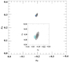 |
Fig. 6 Components of the parallax vector as found by the fit excluding Spitzer (in gray) or including Spitzer data (in cyan). Confidence levels at 68% and 95% are given. |
Microlensing parameters for model A including Spitzer data.
4 Source Analysis
The source characterization is important in determining the correct limb darkening profile to be used in the modeling of the light curve and the angular source radius θ*, which provides a physical scale hooked to the Einstein radius. In the case of OGLE-2019-BLG-0033, we have no observations from OGLE in V band. However, we can exploit MOA observations in V and R bands to construct the color-magnitude-diagram shown in the top panel of Fig. 5, in which we can place the source (green) and identify the center of the red clump on the giant branch (red). We have RMOA,Clump = −12.5931 ± 0.0091 and (V − R)MOA,Clump = 1.0543 ± 0.0065, which can be converted to standard Johnson–Cousins magnitudes using the photometric relations by Bond et al. (2017):
 (11)
(11)
 (12)
(12)
Hence, we obtain IClump = 15.2241 ± 0.0095 and (V − I)Clump = 1.6872 ± 0.0074. Comparing to the Red Clump intrinsic magnitude, IClump,O = 14.384 ± 0.040 (Nataf et al. 2013), and color, (V − I)Clump,O = 106 ± 0.07 (Bensby et al. 2011), at the Galactic coordinate of our microlensing event, we find a reddening of E(V − I) = 0.627 and an extinction AI = 0.852.
The best microlensing model indicates that the blending fraction is compatible with zero, so we attribute the baseline flux entirely to the source, as shown in Fig. 5. Applying the same transformations to the source flux and taking into account the extinction and reddening just derived, we obtain (V − I)*,0 = 1.137 ± 0.071 and I*,0 = 14.835 ± 0.042. Following Yoo et al. (2004), we transform the (V, I) bands to (V, K) bands using the relations by Bessell & Brett (1988) and then find the angular radius of the source following Kervella et al. (2004):
 (13)
(13)
The parallax from Gaia EDR33 for our source is πS = −0.013 ± 0.089 mas, thus it is compatible with zero within the errors (Gaia Collaboration 2016, 2021). So, for an estimate of the source distance, we solely rely on the CMD. As the source position in the CMD is very close to the bulge red clump, it is reasonable to assume it is a bulge giant. Therefore, adopting the Galactic model by Dominik (2006) for the Galactic coordinates of OGLE-2019-BLG-0033, we find that the peak stellar density in the bulge along the observation cone is encountered at a distance DS = 8.1 kpc, which we assume to be a valid proxy for the source distance as well. The uncertainty in the source distance is assumed to be 1 kpc, reflecting the FWHM of the stellar density distribution along the line of sight.
In order to estimate the limb darkening coefficients for our source, we simulate a stellar population with IAC-Star (Aparicio & Gallart 2004) with the stellar evolution library by Bertelli et al. (1994) and the bolometric correction by Castelli & Kurucz (2003). The best match with our source magnitude and color is found for Teff = 4950 K, log g = 2.77 and Z = 0.011. Using the tables by Claret & Bloemen (2011), we get the linear limb darkening coefficients in the relevant bands: uI = 0.5015, uR = 0.5983, and uV = 0.6945. These coefficients have been used to obtain the microlensing models presented in Sect. 3.
5 Lens System Properties
5.1 Mass and Distance
For OGLE-2019-BLG-0033, we benefit from the optimal circumstance in which the lens model is singled out without any degeneracies and with very accurate values for the parallax and source size parameters. In addition, the source is a red clump giant with negligible blending flux, which allows for an easy derivation of the angular source radius that is useful in fixing the Einstein radius as:
 (14)
(14)
By inversion of Eqs. (1) and (4), we can calculate the total mass and the distance to the lens:
 (15)
(15)
 (16)
(16)
where πS = au/DS is the source parallax.
The masses of the two components of the binary lens can be found by use of the mass ratio, q, which is very precisely fixed by the microlensing model: M1 = M/(1 + q) and M2 = qM/(1 + q). Finally, the projected separation of the two lenses can be obtained as
 (17)
(17)
The results of our analysis are reported in Table 4, showing that the binary system is composed of a red dwarf of 0.14 M⊙ and a BD of 0.046 M⊙ at a projected separation of 0.58 au. The light from the system is very weak compared to the background microlensed source, namely, V ~ 26 for a M5V red dwarf, as follows from Benedict et al. (2016), which is in agreement with the negligible blending flux found in the model. The separation of half-au is quite typical for binary systems discovered through the microlensing method as the sensitivity to companions is maximized for separations of the same order as the Einstein radius.
Parameters of the binary lens system.
5.2 Orbital Motion
We have seen that orbital motion was detected for our lens at least in the component along the binary lens axis. In microlens-ing events, a change in the separation s is reflected in rapid evolution of the caustics, which leave an immediate imprint on the light curve. Therefore, it is expected that the component γ1 = (ds/dt)/s is best constrained. The rotation of the axis γ2 = dα/dt is compatible with zero at 1σ level, while for the radial component of the velocity we only have an upper limit, as typical in most microlensing events. With this scarce information, we may still check that the system is really bound by comparing the projected kinetic energy to the potential energy, that is, a bound system must have:
 (18)
(18)
Using the values for our lens system, we find K = 0.0153, which satisfies the constraint, but remains relatively smaller than typical expectations from a random distribution of orbits. Such small values indicate a nearly edge-on orbit, which would apply to our case, given that γ2/γ1 = 0.09. So, with the information in hand, we can conclude that the orbital motion suggested by the light curve fit is perfectly acceptable and consistent with the constraints on the mass and scale of the system coming from the combination of parallax and finite source effects.
5.3 Lens Kinematics
With the determination of the Einstein radius θE (14), we can find the relative lens-source proper motion from Eq. (3) as
 (19)
(19)
which is relatively slow for a lens in the disk (Han & Chang 2003). The components in the eastern and northern directions in the geocentric frame can be derived from the parallax vector:
 (20)
(20)
These can be easily transformed to the heliocentric frame using the velocity components of the Earth at time t0 projected orthogonally to the line of sight:
 (21)
(21)
Thanks to the Gaia EDR3 measurement of the proper motion of the source, we are equipped to carry out a full investigation of the lens kinematics and assign the lens to a distinct component of the Milky Way (Gaia Collaboration 2016, 2021). From Gaia, we have
 (22)
(22)
with components given in the eastern and northern directions, respectively. Then, we can extract the lens proper motion:
 (23)
(23)
We then rotate this vector by 61.36° so as to measure its components in a Galactic frame:
 (24)
(24)
Here, the first component is along the Galactic longitude direction l and the second component is along the Galactic latitude b. As we know the distance of the lens (Eq. (16)), we can translate the proper motion to the velocity components:
 (25)
(25)
Finally, subtracting the peculiar velocity of the Sun, we may move to the local standard of rest (LSR):
 (26)
(26)
Since the line of sight is very close to the Galactic center, these components are very close to the peculiar velocity components of the lens along the tangential circle, v, and orthogonal to the Galactic plane, w, respectively. A value of v ~ −71 km s−1 is quite typical of red metal-poor old stellar populations from the thick disk, as can be inferred from studies of the asymmetric drift (Golubov et al. 2013). So, the kinematic study allows us to firmly assign our lens, made up of a red and a brown dwarf, to Population II stars in the thick disk. Similar conclusions were obtained by Gould (1992), proving the effectiveness of microlensing in the investigation of populations of very low-mass components of our Galaxy.
6 Discussion
6.1 High-Precision Mass Measurements by Microlensing
There is a good number of systems similar to OGLE-2019-BLG-0033 that have been discovered in binary microlensing events, showing that such low-mass binary systems are very common in the Milky Way (Ranc et al. 2015). It is interesting to compare the precision of the mass measurement for our BD to that achieved in other similar microlensing events. Table 5 collects the masses and the relative uncertainties of some microlensing events with binary lenses containing a BD. These events have been selected by us as featuring an uncertainty lower than 10% in the BD mass. We can then realize that our measurement is well-ranked as one of the most precise ever realized for a BD in a binary system.
OGLE-2019-BLG-0033 represents an apt example for demonstrating the potential of microlensing observations to contribute data to a more detailed knowledge of the properties and statistics of low-mass objects in our Galaxy, from planets to BDs and red dwarfs, but also stellar remnants (Blackman et al. 2021; Wyrzykowski & Mandel 2020). Nevertheless, obtaining a unique lens model without degenerate alternatives and with very precise values for the parameters is not that simple. The case of OGLE-2019-BLG-0033 shows that long events with clear parallax and orbital motion signals are optimal for at least two reasons: a precise parallax detection gives a mass-distance relation to be combined with other constraints on θE ; orbital motion may distinguish otherwise degenerate solutions and help single out the correct model. Short events, instead, are typically affected by discrete degeneracies that leave several alternative interpretations for the lens geometry with typically different values for the masses in spite of individual low uncertainties for the degenerate models (Shvartzvald et al. 2016; Mróz et al. 2020). However, annual parallax measurements rely on long-term modulations in the observed flux for which there might be possible alternative explanations or contaminants, including lens orbital motion itsef, xallarap, long-term variability of the source, or sys-tematics in the data. Therefore, the presence of measurements from a different point of observation such as Spitzer, allows for an independent determination of parallax that goes back to pure geometry rather than subtle modulations in the photometry. In fact, Spitzer observations contribute to a further reduction with regard to the uncertainty inherent in our best model.
The second ingredient needed to obtain a precise mass measurement is a good estimate of the Einstein angle, θE. In the case of OGLE-2019-BLG-0033, this is obtained through the detection of finite source effects in the light curve. Although the source did not cross any caustics, it was big enough that even a close approach with the cusps was sufficient to obtain a precise value for ρ*. In addition, the source was a red clump giant with no blending, which made the source analysis particularly easy and precise. The importance of the source analysis should not be underestimated in microlensing mass measurements. Indeed, even in our optimal situation, θ* dominates the error budget in the derived masses. One way to improve the source knowledge could be a systematic spectroscopic survey of bright sources of microlensing events, which certainly may enhance the significance of microlensing mass measurements (Bensby et al. 2010, 2011, 2021). An alternative to finite-source effects, namely, precise mass-distance relations, can be obtained by high-resolution imaging, which works in a complementary way to the annual parallax, as it privileges fast-moving lenses (Bhattacharya et al. 2018), but requires sufficiently bright lenses; otherwise, only the upper limits can be obtained. Measurements of θE have been recently obtained by interferometry (Dong et al. 2019; Cassan et al. 2021), which may open very interesting perspectives for very bright sources. Finally, the astrometric detection of the cen-troid motion provides an alternative channel for space missions (Klüter et al. 2020; Sahu et al. 2022; Lam et al. 2022).
Binary microlensing events with relative error less than 10% for the BD mass.
6.2 The Microlensing Contribution to the Understanding of Brown Dwarfs
There have been more than 3000 BDs discovered to date, and many of them are in the solar neighborhood (Meisner et al. 2020), with some discovered in young clusters (Miret-Roig et al. 2022) and some in binary systems. For FGK stars, the absence of BDs in a close orbit <5AU has led to the postulation of a BD desert (Grether & Lineweaver 2006). Our lens OGLE-2019-BLG-0033 consists of a low-mass M-dwarf as a primary and a BD as a companion with projected separation of 0.587 au. There are many theories explaining the formation of BD binaries: for instance, Offner et al. (2010) describes the formation of low-mass binaries via turbulent fragmentation with separations up to 104 au. Fontanive et al. (2019) posit that there should be a wide-orbit companion for a low-mass star having a close-in orbiting BD; such a wide orbit companion would play a central role in the formation of the BD and also for the sparse population of BDs in close-in orbits (Irwin et al. 2010). Since low-mass binaries are difficult to observe directly, microlensing will play an increasingly important role in identifying such systems, especially with regard to measuring the masses of BDs in binaries and quantifying their occurrence throughout the Galaxy. Kinematic studies combining relative lens-source proper motions from microlensing and source proper motion from Gaia provide very interesting perspectives for assigning low-mass systems to the correct dynamical component of the Galaxy and understanding how the production of BDs may have evolved during the history of the Milky Way.
One of the goals of the upcoming Roman Galactic Exoplanet Survey (RGES) is the determination of the planetary mass function at 10% per decade (Penny et al. 2019; Johnson et al. 2020). By combining high-resolution imaging together with the space parallax and precise characterization of resolved sources, this space mission is likely to provide a substantial census of BDs, including both isolated ones and those in binary systems. Some additional detections are also expected by the xallarap effect (Miyazaki et al. 2021). In order to exploit all this potential, it is necessary to pay adequate attention to equal-mass binary-lens events, even if it is clear that they do not lead to the discovery of planets.
Compared to the BD science from the James Webb Space Telescope (JWST) (Ryan & Reid 2016), Roman has a 100 times wider field of view, enabling the possibility of direct detection of a great number of BDs as a byproduct of its survey operations as a whole, in addition to those that will be detected through microlensing. Instead, JWST will be well-suited for the detection of BDs and rogue planet search in smaller fields, such as clusters, and for the detailed investigation of nearby BDs.
Finally, in terms of a longer perspective, the Extremely Large Telescope, equipped with advanced Adaptive Optics (Trippe et al. 2010), will be able to provide exquisite astrometry in crowded fields. This would be an extraordinary opportunity to revisit all past microlensing events. In fact, current microlens-ing surveys discover about 100 microlensing binary events every year, with most of them likely composed of low-mass objects. A systematic astrometric investigation of all events would thus build a very broad, detailed, and reliable statistics of binary systems in our Galaxy.
7 Conclusions
Here, we present a full analysis of OGLE-2019-BLG-0033, a microlensing event discovered by the OGLE survey and observed by many ground telescopes and from the Spitzer spacecraft. The event is long enough to allow for accurate parallax and orbital motion measurements, along with a detailed characterization of the bright background source. With these favorable circumstances, we managed to achieve an exceptionally precise mass measurement for the lens system, which turns out to be composed of a 0.149 M⊙ red dwarf and a brown dwarf of 0.0463 M⊙ at a projected separation of 0.585 au. The precision of this mass measurement is 6.8%, which is one of the best ever achieved in microlensing observations. The kinematic analysis shows that this binary system is part of the old metal-poor thick disk component of our Galaxy. We argue that the upcoming Roman Galactic Exoplanet Survey will represent a major advance in our understanding of any class of sub-stellar objects.
Acknowledgements
The MOA project is supported by JSPS KAK-ENHI Grant Number JSPS24253004, JSPS26247023, JSPS23340064, JSPS15H00781, JP16H06287, 17H02871 and 19KK0082 and a Royal Society of New Zealand Marsden Grant MFP-MAU1901. U.G.J. acknowledges funding from the European Union H2020-MSCA-ITN-2019 under Grant no. 860470 (CHAMELEON) and from the Novo Nordisk Foundation Interdisciplinary Synergy Program grant no. NNF19OC0057374. W. Zang, W. Zhu, H.Y. and S.M. acknowledge support by the National Science Foundation of China (grant no. 12133005). This research uses data obtained through the Telescope Access Program (TAP), which has been funded by the TAP member institutes. Work by C.R. was supported by a Research Fellowship of the Alexander von Humboldt Foundation. Work by C.H. was supported by the grants of National Research Foundation of Korea (2020R1A4A2002885 and 2019R1A2C2085965). Work by J.C.Y. was supported by JPL grant 1571564. This work has made use of data from the European Space Agency (ESA) mission Gaia (https://www. cosmos.esa.int/gaia), processed by the Gaia Data Processing and Analysis Consortium (DPAC, https://www.cosmos.esa.int/web/gaia/dpac/consortium). Funding for the DPAC has been provided by national institutions, in particular the institutions participating in the Gaia Multilateral Agreement. This work uses observations made at the Observatorio do Pico dos Dias/LNA (Brazil).
References
- Alard, C. 2000, A&As, 144, 363 [NASA ADS] [CrossRef] [EDP Sciences] [Google Scholar]
- Alard, C., & Lupton, R. H. 1998, ApJ, 503, 325 [Google Scholar]
- Albrow, M. D., Yee, J. C., Udalski, A., et al. 2018, ApJ, 858, 107 [NASA ADS] [CrossRef] [Google Scholar]
- An, J. H., Albrow, M. D., Beaulieu, J. P., et al. 2002, ApJ, 572, 521 [NASA ADS] [CrossRef] [Google Scholar]
- Aparicio, A., & Gallart, C. 2004, AJ, 128, 1465 [NASA ADS] [CrossRef] [Google Scholar]
- Auddy, S., Basu, S., & Valluri, S. R. 2016, Adv. Astron., 2016, 574327 [Google Scholar]
- Batista, V., Gould, A., Dieters, S., et al. 2011, A&A, 529, A102 [NASA ADS] [CrossRef] [EDP Sciences] [Google Scholar]
- Béjar, V. J. S., Martín, E. L., Zapatero Osorio, M. R., et al. 2001, ApJ, 556, 830 [CrossRef] [Google Scholar]
- Benedict, G. F., Henry, T. J., Franz, O. G., et al. 2016, AJ, 152, 141 [Google Scholar]
- Bennett, D. P., Bond, I. A., Udalski, A., et al. 2008, ApJ, 684, 663 [Google Scholar]
- Bensby, T., Feltzing, S., Johnson, J. A., et al. 2010, A&A, 512, A41 [NASA ADS] [CrossRef] [EDP Sciences] [Google Scholar]
- Bensby, T., Adén, D., Meléndez, J., et al. 2011, A&A, 533, A134 [NASA ADS] [CrossRef] [EDP Sciences] [Google Scholar]
- Bensby, T., Gould, A., Asplund, M., et al. 2021, A&A, 655, A117 [NASA ADS] [CrossRef] [EDP Sciences] [Google Scholar]
- Bertelli, G., Bressan, A., Chiosi, C., Fagotto, F., & Nasi, E. 1994, A&As, 106, 275 [NASA ADS] [Google Scholar]
- Bessell, M. S., & Brett, J. M. 1988, PASP, 100, 1134 [Google Scholar]
- Bhattacharya, A., Beaulieu, J. P., Bennett, D. P., et al. 2018, AJ, 156, 289 [NASA ADS] [CrossRef] [Google Scholar]
- Blackman, J. W., Beaulieu, J. P., Bennett, D. P., et al. 2021, Nature, 598, 272 [NASA ADS] [CrossRef] [Google Scholar]
- Bond, I. A., Abe, F., Dodd, R. J., et al. 2001, MNRAS, 327, 868 [Google Scholar]
- Bond, I. A., Bennett, D. P., Sumi, T., et al. 2017, MNRAS, 469, 2434 [Google Scholar]
- Bozza, V. 2000, A&A, 355, 423 [NASA ADS] [Google Scholar]
- Bozza, V. 2010, MNRAS, 408, 2188 [NASA ADS] [CrossRef] [Google Scholar]
- Bozza, V., Dominik, M., Rattenbury, N. J., et al. 2012, MNRAS, 424, 902 [Google Scholar]
- Bozza, V., Bachelet, E., Bartolic, F., et al. 2018, MNRAS, 479, 5157 [NASA ADS] [CrossRef] [Google Scholar]
- Bozza, V., Khalouei, E., & Bachelet, E. 2021, MNRAS, 505, 126 [NASA ADS] [CrossRef] [Google Scholar]
- Bramich, D. M. 2008, MNRAS, 386, L77 [NASA ADS] [CrossRef] [Google Scholar]
- Bramich, D. M., Horne, K., Albrow, M. D., et al. 2013, MNRAS, 428, 2275 [NASA ADS] [CrossRef] [Google Scholar]
- Burrows, A., Marley, M., Hubbard, W. B., et al. 1997, ApJ, 491, 856 [Google Scholar]
- Calchi Novati, S., Gould, A., Yee, J. C., et al. 2015, ApJ, 814, 92 [NASA ADS] [CrossRef] [Google Scholar]
- Cassan, A., Ranc, C., Absil, O., et al. 2021, Nat. Astron. [Google Scholar]
- Castelli, F., & Kurucz, R. L. 2003, in Modelling of Stellar Atmospheres, eds. N. Piskunov, W. W. Weiss, & D. F. Gray, 210, A20 [Google Scholar]
- Choi, J. Y., Han, C., Udalski, A., et al. 2013, ApJ, 768, 129 [NASA ADS] [CrossRef] [Google Scholar]
- Claret, A., & Bloemen, S. 2011, A&A, 529, A75 [NASA ADS] [CrossRef] [EDP Sciences] [Google Scholar]
- Close, L. M., Zuckerman, B., Song, I., et al. 2007, ApJ, 660, 1492 [NASA ADS] [CrossRef] [Google Scholar]
- Dominik, M. 1999, A&A, 349, 108 [NASA ADS] [Google Scholar]
- Dominik, M. 2006, MNRAS, 367, 669 [NASA ADS] [CrossRef] [Google Scholar]
- Dominik, M., Jørgensen, U. G., Rattenbury, N. J., et al. 2010, Astron. Nachr., 331, 671 [NASA ADS] [CrossRef] [Google Scholar]
- Dong, S., Mérand, A., Delplancke-Ströbele, F., et al. 2019, ApJ, 871, 70 [CrossRef] [Google Scholar]
- Elmegreen, B. G. 1997, ApJ, 486, 944 [CrossRef] [Google Scholar]
- Fontanive, C., Rice, K., Bonavita, M., et al. 2019, MNRAS, 485, 4967 [Google Scholar]
- Gaia Collaboration (Prusti, T., et al.) 2016, A&A, 595, A1 [NASA ADS] [CrossRef] [EDP Sciences] [Google Scholar]
- Gaia Collaboration (Brown, A. G. A., et al.) 2021, A&A, 649, A1 [NASA ADS] [CrossRef] [EDP Sciences] [Google Scholar]
- Golubov, O., Just, A., Bienaymé, O., et al. 2013, A&A, 557, A92 [NASA ADS] [CrossRef] [EDP Sciences] [Google Scholar]
- Gould, A. 1992, ApJ, 392, 442 [Google Scholar]
- Gould, A. 1994a, ApJ, 421, L75 [NASA ADS] [CrossRef] [Google Scholar]
- Gould, A. 1994b, ApJ, 421, L71 [NASA ADS] [CrossRef] [Google Scholar]
- Gould, A. 2000, ApJ, 542, 785 [NASA ADS] [CrossRef] [Google Scholar]
- Gould, A., & Yee, J. C. 2012, ApJ, 755, L17 [NASA ADS] [CrossRef] [Google Scholar]
- Gould, A., Udalski, A., Monard, B., et al. 2009, ApJ, 698, L147 [Google Scholar]
- Grether, D., & Lineweaver, C. H. 2006, ApJ, 640, 1051 [Google Scholar]
- Han, C., & Chang, H.-Y. 2003, MNRAS, 338, 637 [NASA ADS] [CrossRef] [Google Scholar]
- Han, C., Jung, Y. K., Udalski, A., et al. 2013, ApJ, 778, 38 [NASA ADS] [CrossRef] [Google Scholar]
- Irwin, J., Buchhave, L., Berta, Z. K., et al. 2010, ApJ, 718, 1353 [Google Scholar]
- Johnson, J. A., Apps, K., Gazak, J. Z., et al. 2011, ApJ, 730, 79 [Google Scholar]
- Johnson, S. A., Penny, M., Gaudi, B. S., et al. 2020, AJ, 160, 123 [NASA ADS] [CrossRef] [Google Scholar]
- Kervella, P., Thévenin, F., Di Folco, E., & Ségransan, D. 2004, A&A, 426, 297 [NASA ADS] [CrossRef] [EDP Sciences] [Google Scholar]
- Kim, S.-L., Lee, C.-U., Park, B.-G., et al. 2016, J. Korean Astron. Soc., 49, 37 [Google Scholar]
- Kim, H.-W., Hwang, K.-H., Gould, A., et al. 2021, AJ, 162, 15 [NASA ADS] [CrossRef] [Google Scholar]
- Klüter, J., Bastian, U., & Wambsganss, J. 2020, A&A, 640, A83 [NASA ADS] [CrossRef] [EDP Sciences] [Google Scholar]
- Koshimoto, N., & Bennett, D. P. 2020, AJ, 160, 177 [NASA ADS] [CrossRef] [Google Scholar]
- Koshimoto, N., Baba, J., & Bennett, D. P. 2021, ApJ, 917, 78 [NASA ADS] [CrossRef] [Google Scholar]
- Lafrenière, D., Doyon, R., Marois, C., et al. 2007, ApJ, 670, 1367 [Google Scholar]
- Lam, C. Y., Lu, J. R., Udalski, A., et al. 2022, AAS J., submitted [arXiv:2202.01903] [Google Scholar]
- Larson, R. B. 1992, MNRAS, 256, 641 [NASA ADS] [CrossRef] [Google Scholar]
- Ma, X., & Zhu, W. 2022, MNRAS, 513, 5088 [NASA ADS] [CrossRef] [Google Scholar]
- Mao, S., & Di Stefano, R. 1995, ApJ, 440, 22 [NASA ADS] [CrossRef] [Google Scholar]
- Marcy, G. W., & Butler, R. P. 2000, PASP, 112, 137 [Google Scholar]
- McLean, I. S., McGovern, M. R., Burgasser, A. J., et al. 2003, ApJ, 596, 561 [Google Scholar]
- Meisner, A. M., Faherty, J. K., Kirkpatrick, J. D., et al. 2020, ApJ, 899, 123 [NASA ADS] [CrossRef] [Google Scholar]
- Miret-Roig, N., Bouy, H., Raymond, S. N., et al. 2022, Nat. Astron., 6, 89 [NASA ADS] [CrossRef] [Google Scholar]
- Miyake, N., Sumi, T., Dong, S., et al. 2011, ApJ, 728, 120 [NASA ADS] [CrossRef] [Google Scholar]
- Miyazaki, S., Johnson, S. A., Sumi, T., et al. 2021, AJ, 161, 84 [NASA ADS] [CrossRef] [Google Scholar]
- Mollière, P., & Mordasini, C. 2012, A&A, 547, A105 [NASA ADS] [CrossRef] [EDP Sciences] [Google Scholar]
- Mróz, P., Udalski, A., Skowron, J., et al. 2017, Nature, 548, 183 [Google Scholar]
- Mróz, P., Udalski, A., Skowron, J., et al. 2019, ApJS, 244, 29 [Google Scholar]
- Mróz, P., Poleski, R., Gould, A., et al. 2020, ApJ, 903, L11 [Google Scholar]
- Nataf, D. M., Gould, A., Fouqué, P., et al. 2013, ApJ, 769, 88 [Google Scholar]
- Offner, S. S. R., Kratter, K. M., Matzner, C. D., Krumholz, M. R., & Klein, R. I. 2010, ApJ, 725, 1485 [Google Scholar]
- Padoan, P., Kritsuk, A., Michael, Norman, L., & Nordlund, A. 2005, Mem. Soc. Astron. Italiana, 76, 187 [NASA ADS] [Google Scholar]
- Penny, M. T., Gaudi, B. S., Kerins, E., et al. 2019, ApJS, 241, 3 [CrossRef] [Google Scholar]
- Poindexter, S., Afonso, C., Bennett, D. P., et al. 2005, ApJ, 633, 914 [NASA ADS] [CrossRef] [Google Scholar]
- Ranc, C., Cassan, A., Albrow, M. D., et al. 2015, A&A, 580, A125 [NASA ADS] [CrossRef] [EDP Sciences] [Google Scholar]
- Refsdal, S. 1966, MNRAS, 134, 315 [NASA ADS] [CrossRef] [Google Scholar]
- Ryan, R. E. J., & Reid, I. N. 2016, AJ, 151, 92 [NASA ADS] [CrossRef] [Google Scholar]
- Ryu, Y.-H., Hwang, K.-H., Gould, A., et al. 2021, AJ, 162, 96 [NASA ADS] [CrossRef] [Google Scholar]
- Sahlmann, J., Ségransan, D., Queloz, D., et al. 2011, A&A, 525, A95 [NASA ADS] [CrossRef] [EDP Sciences] [Google Scholar]
- Sahu, K. C., Anderson, J., Casertano, S., et al. 2022, ApJ, submitted, [arXiv:2201.13296] [Google Scholar]
- Schechter, P. L., Mateo, M., & Saha, A. 1993, PASP, 105, 1342 [Google Scholar]
- Shin, I. G., Han, C., Gould, A., et al. 2012, ApJ, 760, 116 [NASA ADS] [CrossRef] [Google Scholar]
- Shin, I. G., Udalski, A., Yee, J. C., et al. 2018, ApJ, 863, 23 [NASA ADS] [CrossRef] [Google Scholar]
- Shin, I.-G., Yee, J. C., Hwang, K.-H., et al. 2022, AJ, 163, 254 [NASA ADS] [CrossRef] [Google Scholar]
- Shvartzvald, Y., Li, Z., Udalski, A., et al. 2016, ApJ, 831, 183 [NASA ADS] [CrossRef] [Google Scholar]
- Skottfelt, J., Bramich, D. M., Hundertmark, M., et al. 2015, A&A, 574, A54 [NASA ADS] [CrossRef] [EDP Sciences] [Google Scholar]
- Skowron, J., Udalski, A., Gould, A., et al. 2011, ApJ, 738, 87 [Google Scholar]
- Smith, M. C., Mao, S., & Paczynski, B. 2003, MNRAS, 339, 925 [NASA ADS] [CrossRef] [Google Scholar]
- Spezzi, L., Beccari, G., De Marchi, G., et al. 2011, ApJ, 731, 1 [NASA ADS] [CrossRef] [Google Scholar]
- Spiegel, D. S., Burrows, A., & Milsom, J. A. 2011, ApJ, 727, 57 [Google Scholar]
- Sumi, T., Abe, F., Bond, I. A., et al. 2003, ApJ, 591, 204 [NASA ADS] [CrossRef] [Google Scholar]
- Tomaney, A. B., & Crotts, A. P. S. 1996, AJ, 112, 2872 [Google Scholar]
- Trippe, S., Davies, R., Eisenhauer, F., et al. 2010, MNRAS, 402, 1126 [NASA ADS] [CrossRef] [Google Scholar]
- Udalski, A., Szymanski, M. K., & Szymanski, G. 2015, Acta Astron., 65, 1 [Google Scholar]
- Vedantham, H. K., Callingham, J. R., Shimwell, T. W., et al. 2020, ApJ, 903, L33 [Google Scholar]
- Whitworth, A., Bate, M. R., Nordlund, Å., Reipurth, B., & Zinnecker, H. 2007, in Protostars and Planets V, eds. B. Reipurth, D. Jewitt, & K. Keil, 459 [Google Scholar]
- Wozniak, P. R. 2000, Acta Astron., 50, 421 [NASA ADS] [Google Scholar]
- Wyrzykowski, Ł., & Mandel, I. 2020, A&A, 636, A20 [NASA ADS] [CrossRef] [EDP Sciences] [Google Scholar]
- Yee, J. C., Hung, L. W., Bond, I. A., et al. 2013, ApJ, 769, 77 [NASA ADS] [CrossRef] [Google Scholar]
- Yee, J. C., Gould, A., Beichman, C., et al. 2015, ApJ, 810, 155 [NASA ADS] [CrossRef] [Google Scholar]
- Yoo, J., DePoy, D. L., Gal-Yam, A., et al. 2004, ApJ, 603, 139 [Google Scholar]
- Zang, W., Penny, M. T., Zhu, W., et al. 2018, PASP, 130, 104401 [NASA ADS] [CrossRef] [Google Scholar]
http://www.fisica.unisa.it/GravitationAstrophysics/RTModel.htm. RTModel performs Levenberg-Marquardt fitting starting from initial conditions obtained by matching the data to template light curves from a library (Mao & Di Stefano 1995).
All Tables
Comparison of parallax πE and χ2 for our four models if Spitzer data are included or excluded.
All Figures
|
Fig. 1 Light curve of the event OGLE-2019-BLG-0033 showing all observations from different telescopes as described in the text. The black curve is the best microlens-ing model for ground observers, and the red curve is the best model for Spitzer observations, as described in Sect. 3. In the bottom panel, we show the residuals from several models: best model including the parallax and orbital motion, best model with parallax without orbital motion, and best static model without parallax. |
| In the text | |
|
Fig. 2 Zoom on the double-peak region of the light curve. The color-coding for the observations is the same as in Fig. 1. |
| In the text | |
|
Fig. 3 Caustics of the four binary lens models examined in our analysis, with the best model labeled as A. The source trajectories are also shown as seen from Earth observatories (black) and from Spitzer (red). |
| In the text | |
|
Fig. 4 Zoom-in on the caustic of the best binary lens model with the source trajectory. The size of the source is shown by the gray disk. |
| In the text | |
|
Fig. 5 Color-magnitude diagrams using different resources. Top panel: CMD of stars in the 2′ field of the event OGLE-2019-BLG-0033 built from MOA observations. The red dot corresponds to the center of the red clump and the green dot shows the position of the source. Bottom panel: CMD built from I-band observations from OGLE and L-band measurements from Spitzer. |
| In the text | |
|
Fig. 6 Components of the parallax vector as found by the fit excluding Spitzer (in gray) or including Spitzer data (in cyan). Confidence levels at 68% and 95% are given. |
| In the text | |
Current usage metrics show cumulative count of Article Views (full-text article views including HTML views, PDF and ePub downloads, according to the available data) and Abstracts Views on Vision4Press platform.
Data correspond to usage on the plateform after 2015. The current usage metrics is available 48-96 hours after online publication and is updated daily on week days.
Initial download of the metrics may take a while.