| Issue |
A&A
Volume 662, June 2022
|
|
|---|---|---|
| Article Number | A126 | |
| Number of page(s) | 7 | |
| Section | Stellar structure and evolution | |
| DOI | https://doi.org/10.1051/0004-6361/202143010 | |
| Published online | 30 June 2022 | |
GRB 190919B: Rapid optical rise explained as a flaring activity
1
Astronomical Institute (ASU CAS), Ondřejov, Czech Republic
e-mail: This email address is being protected from spambots. You need JavaScript enabled to view it.
2
INAF – Instituto di Astrofisica Spaziale e Fisica Cosmica, Milano, Italy
3
Department of Theoretical Physics and Astrophysics, Masaryk University, Brno, Czech Republic
4
Institute of Physics of Czech Academy of Sciences, Prague, Czech Republic
5
Astronomical Institute, MFF UK, Prague, Czech Republic
6
Instituto de Astrofísica de Andalucía (IAA-CSIC), Granada, Spain
7
Instituto de Astronomía de la UNAM, Ensenada, Baja Cfa., Mexico
8
Circuito Exterior s/n, Ciudad Universitaria, Delg. Coyoacán, México DF, Mexico
9
Faculty of Electrical Engneering (FEL-CVUT), Prague, Czech Republic
Received:
27
December
2021
Accepted:
8
March
2022
Abstract
Following the detection of a long GRB 190919B by INTEGRAL (INTErnational Gamma-Ray Astrophysics Laboratory), we obtained an optical photometric sequence of its optical counterpart. The light curve of the optical emission exhibits an unusually steep rise ∼100 s after the initial trigger. This behaviour is not expected from a ‘canonical’ GRB optical afterglow. As an explanation, we propose a scenario consisting of two superimposed flares: an optical flare originating from the inner engine activity followed by the hydrodynamic peak of an external shock. The inner-engine nature of the first pulse is supported by a marginal detection of flux in hard X-rays. The second pulse eventually concludes in a slow constant decay, which, as we show, follows the closure relations for a slow cooling plasma expanding into the constant interstellar medium and can be seen as an optical afterglow sensu stricto.
Key words: techniques: photometric / gamma-ray burst: individual: GRB190919B
© ESO 2022
1. Introduction
Gamma-ray bursts (GRBs) are undoubtedly the brightest single events occurring at cosmological distances. Their isotropic luminosity may reach up to 1054 erg s−1. A broadly accepted scheme explains the prompt gamma-ray emission as produced by internal dissipation processes within the relativistic ejecta (Piran 2004; Mészáros 2006; Zhang 2007; Kumar & Zhang 2015). The long-lived broadband afterglow emission is then usually described in terms of an interaction of the ultra-relativistic ejecta with the ambient medium (Mészáros & Rees 1997; Sari et al. 1998).
The growing ability of rapid follow-up by both X-ray and optical and near-infrared instruments (large number of both space- and ground-based telescopes) permitted us to see the transition between these two modes. A world of interesting features was found in both optical and X-rays as well as in the relation between the two. In contrast to a rather humdrum afterglow behaviour at later times, in the early light curves one may see the onset of the emission and breaks to steeper or shallower decay and flares (Zaninoni et al. 2013; Swenson et al. 2013; Yi et al. 2017).
In this paper, we present observations of the onset of the afterglow of GRB 190919B and propose an explanation for its far too steeply rising afterglow emission. This is something the relativistic fireball model of an afterglow can not explain.
2. Observations
The long GRB, 190919B was detected by INTEGRAL/IBAS (INTErnational Gamma-Ray Astrophysics Laboratory, INTEGRAL Burst Alert System Winkler et al. 2003; Kuulkers et al. 2021; Mereghetti et al. 2003) on September 19, 2019 at 23:46:40 UT in the southern constellation of The Microscope (Mereghetti et al. 2019).
The event localisation was available within 34.6 s to 1.5′accuracy. This precision permitted rapid ground-based follow-up with a number of telescopes, and soon the optical counterpart was discovered at

(Bolmer 2019), and the redshift was determined from several absorption lines in the afterglow spectrum as z = 3.225 (Pugliese et al. 2019).
As found at the Burst analyser web page1 (Evans et al. 2007, 2009, 2010), GRB 190919B was observed in X-rays for 3 ks by Swift-XRT (X-Ray Telescope) ∼30 ks after the trigger. We adopted the results of the spectral fit for this observation, and for reference copy them in Table 1. A further observation was performed ∼128 ks after trigger, but the signal was too faint to centre a centroid at the object, and the pipeline marks this observation as unreliable. Despite this, the Burst analyser mentions an X-ray decay rate of  based on the two mentioned observing epochs.
Parameters of an X-ray spectral fit of the 3 ks observation by Swift-XRT.
2.1. INTEGRAL
Of the instruments aboard the spacecraft, INTEGRAL/ISGRI (INTEGRAL Soft Gamma-Ray Imager, Lebrun et al. 2003) was the primary detector to provide data for our analysis, and SPI (SPectrometer on INTEGRAL) provided some extra signal to be included in the processing, despite reduced performance due to annealing. The GRB was 8.9° off the main axis of the spacecraft, away from the fields of view of Joint European X-Ray Monitor (JEM-X) and the Optical Monitoring Camera (OMC). The high-energy photon detector PICsIT and the anti-coincidence shield did not provide any useful data either.
We processed the data from the INTEGRAL archive with the standard software (Offline Scientific Analysis, OSA version 11). The GRB consisted of a dim first pulse followed by two bright emission episodes. The overall signficance of the GRB detection is ∼24σ.
The two main pulses have different temporal profiles, including different burst asymmetry in terms of the ratio of the rise time to the decay time. These differences eliminate the scenario of a single pulse being seen twice due to strong gravitational lensing.
The resulting background-subtracted light curve is at Fig. 1. The duration of the burst is T90 = 28.5 ± 0.6 s, and the peak flux in the 1 s window at t0 + 19 s was 351.72 photons s−1. We carefully inspected the ISGRI signal during the following three minutes after trigger and found a hint of emission by T0 + ∼120 s.
 |
Fig. 1. INTEGRAL/ISGRI 20−50 keV and 50−150 keV light curves of GRB 190919B. The vertical lines depict the times of individual flare maxima in the high energy range. The hard energy excess is detected during the second main flare at (t − t0)∼20 s in the 100–200 keV energy range. |
Among the considered spectral models (power law, the Band model, cut-off power law (CPL), and black-body + power-law), the spectrum of the burst is best fit with the CPL model with an extra component necessary to explain a high energy excess at about 220 keV (see Fig. 2). However, the spectral properties of the high-energy component are difficult to constrain due to the low number of counts above 100 keV. The model selection was based on the Akaike information criterion (Akaike 1974), AIC = 2d + C, where d is the number of degrees of freedom of the model and C the cstat Poisson log-likelihood obtained from the fitting routine in xspec. The photon index of the CPL model is α = −0.7 ± 0.3, the peak energy of the spectrum Ep = (2 − α)E0 in the observer frame is 54 ± 9 keV, and the total fluence was 1.75 × 10⁻⁸ erg m−2 s−1 in the energy range of 20−200 keV. The known redshift therefore implies a total isotropic energy of Eiso = 3.6 × 1051 erg. We detected no spectral lag in either of the two bright pulses with an estimated upper limit of τ < 150 ms.
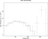 |
Fig. 2. INTEGRAL/ISGRI (20–250 keV) spectrum fit with a CPL model. |
To summarise, INTEGRAL saw GRB 190919B as a relatively faint and soft long GRB typical in most of its aspects. An exception to this is a possible detection of a high energy spectral component at ∼200 keV.
2.2. Ground-based optical
The robotic FRAM (Ph/Fotometric Robotic Atmospheric Monitor) telescope is run by the Institute of Physics of the Czech Academy of Sciences in Prague and is primarily used to monitor atmospheric transparency at the Pierre Auger Observatory in Argentina (Aab et al. 2021). In the case of reception of a gamma-ray-burst satellite alert (Barthelmy et al. 1995), the system is automatically repointed towards it and obtains a pre-defined set of exposures of the burst sky location. Since its installation in 2005, the telescope has observed tens of such alerts, with a few notable optical afterglow detections, such as the 10.2 mag afterglow of GRB 060117, one of the brightest afterglows ever detected (Jelínek et al. 2006). The hardware configuration has changed several times, but at the moment of GRB 190919B it consisted of a 0.3 m telescope with a 60′ × 60′ field of view and a 7° ×7° wide-field camera.
On September 19, 2019 at 23:46:58.0 UT – 34.6 s after the GRB trigger – the INTEGRAL/IBAS (Mereghetti et al. 2019) alert n. 8377.0 was received, the telescope interrupted observations, started to slew, and 53.5 s after the burst at 23:47:16.9 UT it started obtaining a set of 20 s unfiltered exposures; then, it continued with a set of 60 s R-band frames. The CCD camera of the FRAM telescope was set up so that it would read out only the central part of the chip with binning 2 × 2. The images have resolution of 1024 × 1024 pixels and a 30′ × 30′ field of view. The observations were promptly reported (Jelínek et al. 2019).
Furthermore, 3.33 h after the trigger, the 60 cm BOOTES-5/JGT (Burst Observer and Optical Transient Exploration System, Javier Gorosabel Telescope) robotic telescope at Observatorio Astronómico Nacional of San Pedro Martir automatically responded and obtained 64 × 60 s unfiltered exposures. Later, we observed the same afterglow with the BOOTES-3/Yock-Allen telescope at New Zealand (Castro-Tirado et al. 2012). The observation started ∼9 h after the gamma-ray burst and obtained two sets of 60 s unfiltered exposures. The preliminary analysis of the two BOOTES observations was published by Hu et al. (2019). Full observation logs are listed in Table 2.
Photometric measurements of the optical afterglow of GRB 190919B.
3. Analysis
In the earliest images (except the first two), the afterglow was detectable in single exposures, and after ∼20 min it disappeared; however, by co-adding the exposures, it was possible to detect it until 120 min post trigger. By co-adding images from the telescope BOOTES-3, we were able to detect the optical source as late as 9.54 h after the GRB, allowing us to better estimate the temporal decay rate.
An identification chart with the optical afterglow of GRB 190919B marked is shown in Fig. 3, and the obtained photometric points are listed in Table 2. However, in order to properly treat low fluxes and errors, we did not use the FRAM points for fitting; instead, we blindly measured signal within the aperture in every single frame and performed the fitting with many imprecise points rather than few precise ones. This means that we did not follow the common add – detect – centre – measure procedure used for CCD photometry of faint astronomical objects. This procedure also permits us to use a robust fitting algorithm to identify and ignore frames that might otherwise influence the co-added photometric signal. The light-curve fitting was performed in linear space (i.e. not in the logarithmic magnitude space) with these points (see Fig. 4). The light curve from both telescopes complemented with the photometric points collected from GCN circulars is shown in Fig. 5.
 |
Fig. 3. Image of the optical afterglow of GRB 190919B obtained by the telescope FRAM, this image shows 10′ × 10′ with north up and east to the left. The 1.5′ INTEGRAL/IBAS error box is marked with a circle. |
 |
Fig. 4. Optical light curve of GRB 190919B, fitted with an empirical model consisting of a superposition of two smoothly broken power-law functions (see Sect. 3.1) to describe two pulses as discussed in Sect. 4. |
 |
Fig. 5. Optical light curve of GRB 190919B in log-log plot in which the used power laws show as straight lines. The fitted, smoothly broken power-law pulse functions (blue, red) take the form of a hyperbola. The final model is a superposition of these two pulses (black line). The points shown are the photometric points from Table 2. We note that the fitting was performed in linear space and with single-image fluxes, as shown in Fig. 4. |
The earliest images from FRAM were obtained before the afterglow reached its maximum brightness. The maximum can be seen by about 120–420 s and reaches ∼16.5 mag. From 600 s on, only a simple power-law decay is observed.
To quantify the possible host-galaxy contamination of the observed photometric data, we searched for a host in the archive images of the Legacy survey (Dey et al. 2019). There seems to be no detection with an estimated limit in the range of r′∼25. The faintest known GRB 190919B afterglow detection with r′=21.48 by Strausbaugh & Cucchiara (2019) should therefore have at most 4% light from the host.
3.1. Light-curve fitting
In order to characterise the complex shape of the optical light curve shown in Fig. 4, we fitted it with an empirical model consisting of two smoothly broken power-law functions of the following form:
 (1)
(1)
which peaks at t = T0 and shows the asymptotic behaviour of power laws with slopes of α1 and α2 to the left and right of the peak, respectively. The smoothing parameter Δ defines how sharp the transition is between the two power-law segments. In our analysis, we assumed, for simplicity, that this smoothing parameter is the same for both peaks. We also assumed uniform priors with reasonable limits (see Table 3) for all the parameters of the resulting model. Finally, we used Goodman \AMP Weare’s affine invariant Markov chain Monte Carlo (MCMC) ensemble sampler (Goodman & Weare 2010) implemented by the Python package EMCEE (Foreman-Mackey et al. 2013) to explore the parameter space. To ensure fit convergence, we allowed the MCMC to run until the number of steps exceeded one hundred times the maximum of the auto-correlation length of all parameters. Then, we used 5%, 50%, and 95% quantiles of marginalised parameter distributions in the samples to derive their best fit values and 90% confidence limits. The resulting regions of acceptable parameters are shown in Fig. 6 and summarised in Table 3. Figure 4 shows the model corresponding to best fit parameters overplotted on the data used for the fit. Reduced χ2 of this model is 1.29 (for 116 degrees of freedom), thus ensuring that the model is indeed adequate to the data, and the confidence limits mentioned above are reliable.
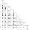 |
Fig. 6. Parameters for the empirical model fitting of the light curve with two smoothly broken power laws as described in Sect. 3.1. |
3.2. Spectral energy distribution
Using the fitted temporal behaviour, we combined the available data from 407 s (infrared (IR) observations, Bolmer 2019), 34 ks (Swift X-ray, Evans et al. 2007, 2009, 2010), and 67 ks (late r′+ i′, Strausbaugh & Cucchiara 2019) to create a SED of the afterglow emission (see Table 4).
Photometric measurements of the optical afterglow collected from GCN circulars.
The X-ray data we used (see Table 1) were corrected for interstellar hydrogen absorption using the hydrogen absorption column NH = 2.75 × 1020 cm−2. The optical data were also corrected for the Galactic dust absorption according to the Galactic reddening maps of Schlegel et al. (1998). Both X-ray and optical data were converted to the same units of measurement (janskys) for the purpose of comparison.
Despite the relative distance between the three epochs, a common, simple power-law spectrum can be constructed. We fitted the optical and IR points for dust extinction in the host galaxy, which we approximated using the values adopted from Cardelli et al. (1989). Under the assumption that the broadband spectrum is a simple power law, we obtained a rough estimate of the dust reddening of E(B − V)=0.28 ± 0.05, together with a spectral slope of βfit = 1.05 ± 0.07. This result is in agreement with both the X-ray spectrum and the expected spectral slope of β = 2α/3 + 1/2 = 1.05, as derived from the fitted late temporal decay rate α2, 2 (see Fig. 7).
 |
Fig. 7. Spectral energy distribution (SED) of GRB 190919B afterglow. Three different epochs were collapsed to provide the most comprehensive image available. The optical points were scaled so that they would represent the afterglow at 34 ks after the trigger. All observations are in agreement with a spectral slope of β = 1.05 derived from a fitted late-decay rate. X-ray point to the right is displayed together with its respective spectral slope and including the slope uncertainty (hence the butterfly). Frequencies are in the observer frame, the optical flux of the afterglow was corrected for Galactic extinction, as was the X-ray spectrum for interstellar hydrogen absorption. The blue optical and infreared points were also corrected for host galaxy dust absorption of E(B − V)=0.28. |
3.3. Search for late, high-energy emission
A careful search for the late, high-energy INTEGRAL/ISGRI emission was performed around the time (t − t0)≈200 s, at which the optical afterglow peaks. A flare-finding algorithm that works with flexible time binning (see Mereghetti et al. 2021) suggested a possible 3.4σ faint detection in the 20–100 keV light curve between 103 s < (t − t0)< 126 s (see Fig. 8). To further investigate the significance of the potential signal, we inspected the distribution of the counts on the detector as a function of pixel illumination fraction (PIF) from the source at the position of GRB 190919B during the time interval selected by the flare-finder routine. The hypothesis of the existence of the signal and the background were tested against the hypothesis with only the background contribution similarly to the method described in Mereghetti et al. (2021) (Rigoselli et al., in prep.). A Bayesian approach using the MCMC fitting yields the significance of the source with 3.11σ, calculated according to  , where λ ≡ ℒ(b)/ℒ(s + b) is the likelihood ratio of the likelihoods of the observed data given the hypothesis with the background only, resp. with the background plus the signal as the underlying model (Li & Ma 1983). Further investigation of the ISGRI detector plane revealed the necessity to correct the counts for a bad pixel that escaped the OSA bad pixel selection filter. This reduced the significance of the detection to 2.96σ.
 |
Fig. 8. Possible, faint, ∼3σ flare highlighted by the flare-finding algorithm applied blindly on the light curve of GRB 190919B in the 20–100 keV energy range with a coarse binning of 4 s. |
For comparison, the GRB itself within the duration of the T90 had a significance of 23.9σ, while randomly selected regions of the same duration as the late emission candidate containing no clear signal at different times before and after the flare showed only a 0.06−0.10σ detection at best using this method. Using a rough estimate of ∼25 μJy at ∼50 keV for this emission, we obtain a spectral slope of 0.3, which is significantly harder than that of the later optical afterglow.
4. Discussion
4.1. The first pulse
Our preferred interpretation of the steep rising and the first pulse is an ongoing activity of the internal engine. This way, we obtain a simple explanation for the steep rise – the flare would follow its own time frame and it would not be bound to the shell dynamic of the afterglow.
The contemporaneous X-ray and optical peaks point towards a common origin similar to that of an XRF 071031 (Krühler et al. 2009); this was also a soft GRB, and the spectral X-rays-to-optical ratio was similar (βX − opt ∼ 0.3). The similarity makes us believe that what we have seen was, in fact, a late activity of the inner engine, which, with time, slowly softens and shifts its spectral peak towards longer wavelengths.
A competing interpretation for this pulse may be a reverse shock (RS) emission related to the later-observed afterglow, and while it cannot be completely disregarded, it is disfavoured by the ISGRI hard X-ray detection. Also, the RS timescale is expected to be different – it is expected to start rising immediately when the ejecta hits the interstellar matter (ISM) (Zhang et al. 2003) – that is earlier than observed. The temporal index of the rise of this pulse (α1, 1 ≃ 5.2 with respect to T0) is also steeper than expected for a reverse shock emission (Sari & Piran 1999).
On the other hand, Martin-Carrillo et al. (2014) observed a strong optical pulse at a similar time, coincident with the end of the gamma-ray emission for a much brighter GRB 120711A, and interpreted it as a reverse shock emission. So, while noting that the high-energy emission related to our pulse is much weaker, a RS+FS scenario similar to their interpretation is also possible. While we prefer the scenario of the broadband optical+X-ray flaring activity, a definitive decision on the nature of the pulse is impossible with the available data.
4.2. The second pulse and closure relations
For the second fitted pulse, we propose an interpretation of a hydrodynamic maximum of an expanding-shell afterglow emission. For the optical afterglows as interpreted by the relativistic fireball model, the emission during the decay depends on time and frequency as F ∼ tανβ, where the indexes β and α are bound together with an electron distribution parameter p (which itself depends on microphysical parameters). The precise relations for the α and β parameters depend, however, on the regime of the shockwave and the medium-density profile it is spreading into.
The rising temporal index of this pulse α1, 2 ≃ 2.1 is a value expected for a rising edge of an optical afterglow. Our fitted final optical decay is α2 = 0.81 ± 0.10. If this decay represents slow-cooling ejecta expanding into constant density profile, following Sari et al. (1998) we could expect this decay to be related with the value of the electron-distribution index p as α = 3(1 − p)/4. with p = 2.08 ± 0.13. The Swift-XRT photon index βX = 1.1 agrees well with the model relation β = p/2. Furthermore, with a host extinction E(B − V)host = 0.28 (see Sect. 3.2), the X-ray-to-optical spectral slope becomes perfectly compatible with the spectral slope β = 1.05 derived from the afterglow theory.
As noted above, the late Swift-XRT observation obtained 128 ks post-burst is considered unreliable as it is too weak. The associated values of the decay rate of  and the X-ray-to-optical spectral slope of βOX, late = 0.99 may point towards a change of regime, but deeper inspection of the late-time behaviour is impossible with the available data.
Testing other possible combinations of conditions (fast cooling, wind profile, post jet-break decay) provides unrealistically low values of p ≪ 2 and no compatibility between spectral and optical indices.
4.3. Initial gamma factor
For the fitted values, we can estimate the initial Lorentz factor of the ejecta Γ0 (similarly to Molinari et al. 2007), for which we have:
 (2)
(2)
where
![Mathematical equation: $$ \begin{aligned} \Gamma (t_\mathrm{peak} ) \approx 160 \left[ \frac{E_{\gamma , 53}(1+z)^3}{\eta _{0, 2} n_0 t_\mathrm{peak,2} ^3} \right]^{1/8}, \end{aligned} $$](/articles/aa/full_html/2022/06/aa43010-21/aa43010-21-eq11.gif) (3)
(3)
Eγ = Eγ, 531053 erg is the overall isotropic energy, and tpeak, 2 = tpeak/100 s is a corrected time of the maximum. The values η0, 2 and n0 are unknown but are assumed to be close to unity and the resulting Lorentz factor depends only weakly on them. Using the fitted value of  s and the isotropic energy of Eiso = 3.6 × 1051 erg, we obtain the initial Lorentz factor value of Γ0 = 250, in agreement with values expected for the relativistic fireball model (Γ0 in range of 50 to 1000, see Piran 2000).
5. Conclusions
GRB 190919B was a 26 s gamma-ray burst detected at a redshift of z = 3.225 by INTEGRAL. It consisted of one faint and two bright gamma-ray pulses, followed by a marginally significant hint of a flaring event ∼120 s post-trigger. The spectrum of the burst was relatively soft, but shows an apparent excess of gamma-ray emission at 200 keV during the brightest pulse.
Following its localisation, we obtained early photometry of the optical afterglow with three robotic telescopes: FRAM, BOOTES-3, and BOOTES-5. The data we collected permitted us to construct a light curve of the afterglow, and, complemented with publicly available information, we were also able to construct its spectral energy distribution. The optical light curve rose steeply ∼100 s after the trigger (almost 10× in brightness), and eventually it reaches a maximum of 16.5 mag. The light curve then started to become fainter and settles at a power-law decay rate of α2 = 0.81 ± 0.10 until it faded away.
We interpret the steeply rising afterglow light curve as the superposition of two pulses of different physical natures. The first pulse can be plausibly interpreted as a flare corresponding to internal engine activity. This scenario is supported by a hint of hard X-ray emission detected simultaneously to the fitted pulse in the INTEGRAL/ISGRI data.
The second pulse is interpreted similarly to other GRBs as an onset of the afterglow emission and a forward shock (FS) of an ejecta colliding with a constant density interstellar matter. The initial gamma factor corresponding to the delay between the GRB trigger and the peak of the emission is Γ0 ≈ 250. The late afterglow decay and X-ray-to-optical spectrum is consistent with the prediction of the relativistic fireball model with an expansion in the slow-cooling regime into a constant density interstellar medium with an electron distribution parameter of p = 2.08 ± 0.13.
Acknowledgments
We would like to thank the Pierre Auger Collaboration for the use of its facilities. Further, we would like to thank the Lauder Atmospheric Research Station and Dr. Richard Querel for hosting and support of BOOTES-3. The operation of the robotic telescope FRAM is supported by the grant of the Ministry of Education of the Czech Republic LM2018102. The data calibration and analysis related to the FRAM telescope is supported by the Ministry of Education of the Czech Republic MSMT-CR LTT18004, MSMT/EU funds CZ.02.1.01/0.0/0.0/16_013/0001402 and CZ.02.1.01/0.0/0.0/18_046/0016010. SK and MP acknowledge support from the European Structural and Investment Fund and the Czech Ministry of Education, Youth and Sports (Project CoGraDS – CZ.02.1.01/0.0/0.0/15_003/0000437). MT and MR acknowledge support from the Ministry of Education and Research of Italy via project PRIN-MIUR 2017 UnIAM (Unifying Isolated and Accreting Magnetars). YDH acknowledges support under the additional funding from the RYC2019-026465-I. AJCT acknowledges support from the Spanish Ministry Project PID2020-118491GB-I00 and the “Center of Excellence Severo Ochoa” award for the Instituto de Astrofísica de Andalucía (SEV-2017-0709) as well as technical support from both NIWA Lauder and San Pedro Mártir Astronomical Observatory staff. We would also like to thank an anonymous referee for helpful comments that improved the quality of the paper.
References
- Aab, A., Abreu, P., Aglietta, M., et al. 2021, JINST, 16, P06027 [Google Scholar]
- Akaike, H. 1974, IEEE Trans. Autom. Control, 19, 716 [Google Scholar]
- Barthelmy, S. D., Butterworth, P., Cline, T. L., et al. 1995, Ap&SS, 231, 235 [NASA ADS] [CrossRef] [Google Scholar]
- Bolmer, J. 2019, GCN Circ., 25789 [Google Scholar]
- Cardelli, J. A., Clayton, G. C., & Mathis, J. S. 1989, ApJ, 345, 245 [Google Scholar]
- Castro-Tirado, A. J., Jelínek, M., Gorosabel, J., et al. 2012, Astron. Soc. India Conf. Ser., 7, 313 [Google Scholar]
- Dey, A., Schlegel, D. J., Lang, D., et al. 2019, AJ, 157, 168 [Google Scholar]
- Evans, P. A., Beardmore, A. P., Page, K. L., et al. 2007, A&A, 469, 379 [NASA ADS] [CrossRef] [EDP Sciences] [Google Scholar]
- Evans, P. A., Beardmore, A. P., Page, K. L., et al. 2009, MNRAS, 397, 1177 [Google Scholar]
- Evans, P. A., Willingale, R., Osborne, J. P., et al. 2010, A&A, 519, A102 [NASA ADS] [CrossRef] [EDP Sciences] [Google Scholar]
- Foreman-Mackey, D., Hogg, D. W., Lang, D., & Goodman, J. 2013, PASP, 125, 306 [Google Scholar]
- Goodman, J., & Weare, J. 2010, Commun. Appl. Math. Comput. Sci., 5, 65 [Google Scholar]
- Hu, Y.-D., Fernandez-Garcia, E., Castro-Tirado, A. J., et al. 2019, GCN Circ., 25798 [Google Scholar]
- Jelínek, M., Prouza, M., Kubánek, P., et al. 2006, A&A, 454, L119 [NASA ADS] [CrossRef] [EDP Sciences] [Google Scholar]
- Jelínek, M., Karpov, S., Mašek, M., et al. 2019, GCN Circ., 25794 [Google Scholar]
- Krühler, T., Greiner, J., McBreen, S., et al. 2009, ApJ, 697, 758 [CrossRef] [Google Scholar]
- Kumar, P., & Zhang, B. 2015, Phys. Rep., 561, 1 [Google Scholar]
- Kuulkers, E., Ferringo, C., Kretschmar, P., et al. 2021, New Astron. Rev., 93, 101629 [CrossRef] [Google Scholar]
- Lebrun, F., Leray, J. P., Lavocat, P., et al. 2003, A&A, 411, L141 [NASA ADS] [CrossRef] [EDP Sciences] [Google Scholar]
- Li, T. P., & Ma, Y. Q. 1983, ApJ, 272, 317 [CrossRef] [Google Scholar]
- Martin-Carrillo, A., Hanlon, L., Topinka, M., et al. 2014, A&A, 567, A84 [NASA ADS] [CrossRef] [EDP Sciences] [Google Scholar]
- Mereghetti, S., Götz, D., Borkowski, J., Walter, R., & Pedersen, H. 2003, A&A, 411, L291 [NASA ADS] [CrossRef] [EDP Sciences] [Google Scholar]
- Mereghetti, S., Gotz, D., Ferrigno, C., et al. 2019, GCN Circ., 25788 [Google Scholar]
- Mereghetti, S., Topinka, M., Rigoselli, M., & Götz, D. 2021, ApJ, 921, L3 [NASA ADS] [CrossRef] [Google Scholar]
- Mészáros, P. 2006, Rep. Prog. Phys., 69, 2259 [CrossRef] [Google Scholar]
- Mészáros, P., & Rees, M. J. 1997, ApJ, 476, 232 [CrossRef] [Google Scholar]
- Molinari, E., Vergani, S. D., Malesani, D., et al. 2007, A&A, 469, L13 [NASA ADS] [CrossRef] [EDP Sciences] [Google Scholar]
- Piran, T. 2000, Phys. Rep., 333, 529 [CrossRef] [Google Scholar]
- Piran, T. 2004, Rev. Mod. Phys., 76, 1143 [Google Scholar]
- Pugliese, D., Izzo, L., Bolmer, J., et al. 2019, GCN Circ., 25792 [Google Scholar]
- Sari, R., & Piran, T. 1999, ApJ, 520, 641 [NASA ADS] [CrossRef] [Google Scholar]
- Sari, R., Piran, T., & Narayan, R. 1998, ApJ, 497, L17 [Google Scholar]
- Schlegel, D. J., Finkbeiner, D. P., & Davis, M. 1998, ApJ, 500, 525 [Google Scholar]
- Strausbaugh, R., & Cucchiara, A. 2019, GCN Circ., 25796 [Google Scholar]
- Swenson, C. A., Roming, P. W. A., De Pasquale, M., & Oates, S. R. 2013, ApJ, 774, 2 [NASA ADS] [CrossRef] [Google Scholar]
- Winkler, C., Courvoisier, T. J.-L., di Cocco, G., et al. 2003, A&A, 411, L1 [NASA ADS] [CrossRef] [EDP Sciences] [Google Scholar]
- Yi, S.-X., Yu, H., Wang, F. Y., & Dai, Z.-G. 2017, ApJ, 844, 79 [NASA ADS] [CrossRef] [Google Scholar]
- Zaninoni, E., Bernardini, M. G., Margutti, R., Oates, S., & Chincarini, G. 2013, A&A, 557, A12 [NASA ADS] [CrossRef] [EDP Sciences] [Google Scholar]
- Zhang, B. 2007, Chin. J. Astron. Astrophys., 7, 1 [NASA ADS] [CrossRef] [Google Scholar]
- Zhang, B., Kobayashi, S., & Mészáros, P. 2003, ApJ, 595, 950 [NASA ADS] [CrossRef] [Google Scholar]
All Tables
All Figures
|
Fig. 1. INTEGRAL/ISGRI 20−50 keV and 50−150 keV light curves of GRB 190919B. The vertical lines depict the times of individual flare maxima in the high energy range. The hard energy excess is detected during the second main flare at (t − t0)∼20 s in the 100–200 keV energy range. |
| In the text | |
|
Fig. 2. INTEGRAL/ISGRI (20–250 keV) spectrum fit with a CPL model. |
| In the text | |
|
Fig. 3. Image of the optical afterglow of GRB 190919B obtained by the telescope FRAM, this image shows 10′ × 10′ with north up and east to the left. The 1.5′ INTEGRAL/IBAS error box is marked with a circle. |
| In the text | |
|
Fig. 4. Optical light curve of GRB 190919B, fitted with an empirical model consisting of a superposition of two smoothly broken power-law functions (see Sect. 3.1) to describe two pulses as discussed in Sect. 4. |
| In the text | |
|
Fig. 5. Optical light curve of GRB 190919B in log-log plot in which the used power laws show as straight lines. The fitted, smoothly broken power-law pulse functions (blue, red) take the form of a hyperbola. The final model is a superposition of these two pulses (black line). The points shown are the photometric points from Table 2. We note that the fitting was performed in linear space and with single-image fluxes, as shown in Fig. 4. |
| In the text | |
|
Fig. 6. Parameters for the empirical model fitting of the light curve with two smoothly broken power laws as described in Sect. 3.1. |
| In the text | |
|
Fig. 7. Spectral energy distribution (SED) of GRB 190919B afterglow. Three different epochs were collapsed to provide the most comprehensive image available. The optical points were scaled so that they would represent the afterglow at 34 ks after the trigger. All observations are in agreement with a spectral slope of β = 1.05 derived from a fitted late-decay rate. X-ray point to the right is displayed together with its respective spectral slope and including the slope uncertainty (hence the butterfly). Frequencies are in the observer frame, the optical flux of the afterglow was corrected for Galactic extinction, as was the X-ray spectrum for interstellar hydrogen absorption. The blue optical and infreared points were also corrected for host galaxy dust absorption of E(B − V)=0.28. |
| In the text | |
|
Fig. 8. Possible, faint, ∼3σ flare highlighted by the flare-finding algorithm applied blindly on the light curve of GRB 190919B in the 20–100 keV energy range with a coarse binning of 4 s. |
| In the text | |
Current usage metrics show cumulative count of Article Views (full-text article views including HTML views, PDF and ePub downloads, according to the available data) and Abstracts Views on Vision4Press platform.
Data correspond to usage on the plateform after 2015. The current usage metrics is available 48-96 hours after online publication and is updated daily on week days.
Initial download of the metrics may take a while.