© H. Labriji et al. 2022

1 Introduction

Due to the decrease in the air refractive index with altitude, light rays entering the atmosphere or emitted from Earth are bent, respectively, towards the ground or towards the horizon. This phenomenon, illustrated in Fig. 1, has spatial and temporal consequences. First, the ray is bent towards the ground, making the actual ray differ from the expected ray. The deviation between the two trajectories is characterised by a shift b outside the atmosphere, the computation of which is the main goal of this paper, and a difference in the apparent position of the object at the observer level. The deviation between the true geometric direction (tag (0)) and the apparent optical direction (tag (1)) is the well-known angle of refraction R_a (Mahan 1962; Thomas & Joseph 1996) and depends on the observation wavelength, which causes a visible stretching of the stars ΔR_a, also known as the blur effect. Second, the ray distortion changes the trip time across the atmosphere, which is of interest for satellite ranging systems (Gardner 1977; Dodson 1986; Abshire & Gardner 1985; Marini 1972).

The purely angular correction R_a is well adapted to astrometry, namely when compensating the position of an object optically located at infinity such as a star. However, there are a number of cases where it is necessary to take into account the shift b of the ray with respect to its vacuum path (tag (2)) and its chromatism Δb, as pictured in Fig. 1.

A first case is the correction of atmospheric turbulence over a wide spectral domain. It is usual in adaptive optics to operate the wavefront sensor in a different band than the imaging sensor (Nakajima 2006). Stellar interferometers are also impacted by this issue, as they can operate on different bands, while only one of them is dedicated to the fringe tracker (Pannetier et al. 2021). The chromaticity of the lateral shift (Fig. 1), sometimes called the ‘chromatic shear’ (Nakajima 2006), makes the integrated wavefront error vary with wavelength, creating a ‘chromatic anisoplanatism’ (Devaney et al. 2008; Sasiela 1992) that is not corrected even if an atmospheric dispersion corrector is used to correct dispersion in the focal plane. As it is difficult to correct the impact of refraction, it is mostly considered as part of the residual errors induced by the atmospheric dispersion corrector (van den Born & Jellema 2020).

The second case is estimating the position of an object near Earth using its apparent position in the sky, as typically used in meteor tracking networks (McCrosky & Posen 1968; Jeanne et al. 2019; Gardiol et al. 2021; Colas et al. 2014, 2020; Egal et al. 2017; Vida et al. 2021; Tóth et al. 2015). Since the object is generally observed at an altitude larger than 20 km, its apparent position is affected at low elevations by atmospheric refraction. The all-sky cameras calibrate the position of the identified objects based on the known positions of the stars (Borovicka et al. 1995). Yet, the fact that the object is not at an infinite distance from the observer (unlike the stars) makes this correction unsuitable, and we can see in Fig. 1 that the error is equal to the lateral shift b.

The third example of the shift compensation’s usefulness is the observation of Earth from space. This time, the projection Δ of the lateral shift on the ground (Fig. 1) is used to compensate refraction when estimating the position of the generated data (Yan et al. 2016; Li et al. 2016). Thus, since atmospheric wave-front distortions are much less critical when observing Earth from space than space form Earth, Earth observation satellites can operate at large zenith angle and have their line of sight significantly shifted on the ground.

Atmospheric refraction was recorded in the literature very early, and Aristotle mentions the vertical stretching at the horizon in his book Meteorology (Aristotle 1908), while the first instrumental proof was made by Johannes Schöner and reported in a monograph written by Regiomontanus (1544). The famous Danish astronomer Tycho Brahe was one of the first people to measure the effect of refraction using the apparent position of sun at Earth’s summer and winter solstices (Mahan 1962).

Later, the angle R_a has been the subject of several studies; authors such as Radau (1882), Saastamoinen (1972), and Chambers (2005) have approached the refraction angle with a series of approximations, while others integrated the variation equations of the light path numerically (Hohenkerk & Sinclair 1985; Seidelmann 1992; Stone 1996; Wittmann 1997; Kristensen 1998; Auer & Standish 2000; Nauenberg 2017). In contrast to the refraction angle, the calculation of the lateral shift b has been identified as a difficult problem by McCrosky & Posen (1968), and there have been a few early attempts to approximate it (Schmid 1963). Within the framework of adaptive optics, Wallner has written two papers on this issue (Wallner 1976, Wallner 1977). In Wallner (1976), one can find an expression of the lateral shift (as a function of the altitude h) whose derivation assumes that the Earth is flat: $$b\left(h,\lambda \right)=N_{\text{S}}\left(\lambda \right)\frac{\tan z_{\infty }}{\cos z_{\infty }}\frac{P\left(h\right)}{\mathcal{G}{\rho }_{\text{S}}},$$(1)

where z_∞ refers to the zenith angle of the non-refracted ray, P is the atmospheric pressure at altitude h, g is the standard gravity, ρ_S = 1.225 kg m^–3 is a constant, and N_S(λ) represents the variation of the refractive index with wavelength (λ).

Based on Eq. (1), some authors have continued his work to evaluate wavefront sensing degradation for extremely large telescopes (ELTs) (Owner-Petersen & Goncharov 2004; Owner-Petersen 2006; Jolissaint & Kendrew 2010). Several other papers seem to have independently found and used the same expression of the lateral shift (Sasiela 1992; Nakajima 2006).

This article is dedicated to the calculation of the lateral shift. We begin Sect. 2 by rigorously writing the differential equations in the spherical Earth model. The remaining part of Sect. 2 is devoted to the study of the estimator (denoted b^(∞)) resulting from the numerical integration of the local equations. The evolution of the estimator is also investigated as a function of the observation wavelength and the temperature and pressure conditions. Then, in Sect. 3, we describe our use of a Taylor expansion of the variational equations to deduce three other estimators of the lateral shift b⁽¹⁾ (Eq. (46)), b^(3/2) (Eq. (50)), and b⁽²⁾ (Eq. (43)). We provide the means to calculate their values knowing only the meteorological conditions of the observation site and the distribution of air in the atmosphere. In Sect. 3.5, we study the accuracy of each approximation as a function of the zenith angle. Finally, in Sect. 4 we discuss two applications of the lateral shift. In Sect. 4.1, we start by studying the effect of numerical integration on the ‘chromatic shear’ values in wave-front sensing, and then we focus on the effect of the lateral shift for the observation of nearby objects (Sect. 4.2). Theoretical models for the atmosphere and its moments are described in the appendices. A companion PYTHON program to this article is available¹.

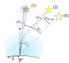Fig. 1 Bending of light rays due to atmospheric refraction.

2 Derivation of the lateral shift in the spherical atmosphere model

2.1 Differential equations from geometric analysis

We consider a ray that reaches the observer at point Ω in a spherical model of Earth’s atmosphere as depicted in Fig. 2. The light ray passes through point M at the altitude h and point N at h + dh. The hypothetical path in absence of atmosphere is represented by a dotted line. We note R_T the Earth’s radius, h the altitude of the point M, n the local refractive index, z the angle that the ray makes at a point M with the direction of the zenith at the observer, ζ the local zenith angle at each altitude, and s the length along the optical path.

The subscript 0 always refers to a quantity measured at ground level (i.e. at the observer level), while the subscript ∞ refers to a quantity at infinity. z₀ is the apparent zenith angle at the observer level, and z_∞ is the angle between the non-refracted ray and the zenith at Ω. The classical refraction angle is denoted R_a and: $$R_{\text{a}}=z_{\infty }-z_0.$$(2)

The variation of the local zenith angle at each altitude h satisfies the Bouguer invariant and depends on the local refractive index as follows: $$R_{\text{T}}{n}_0\sin {\zeta }_0=\left(R_{\text{T}}+h\right)n\sin \zeta .$$(3)

This formula stems from Snell Descartes’ law; its proof can be found in Chapter 6 of Kovalevsky & Seidelmann (2004).

In the following, we derive the equations of variations of the main variables describing the optical path of the light ray: z, ζ, and h. Some of those are already known in the usual computation of the angle of refraction z_∞ – z₀ (Hohenkerk & Sinclair 1985). The goal here is to express the lateral shift b(h) according to given parameters such as the zenith angle. As already highlighted in many references (Kovalevsky & Seidelmann 2004), the main difficulty of this calculation in spherical atmosphere is the continuous change of the zenith direction (ζ) along the ray path. Using the variable z, which represents the angle that the ray makes with the zenith at the point of observation, allows us to overcome this difficulty.

First, differentiating the Bouguer formula, one obtains $$\frac{\text{d}h}{R_{\text{T}}+h}\tan \left(\zeta \right)+\text{d}\zeta =-\frac{\text{d}n}{n}\tan \left(\zeta \right).$$(4)

Then, introducing θ in Fig. 2, one has the following in the OKM triangle: $$z=\zeta +\theta .$$(5)

Moreover, in the MHN triangle (where MH is a circle arc): $$\left(R_{\text{T}}+h\right)\text{d}\theta =\tan \left(\zeta \right)\text{d}h,$$(6)

which implies, combined with Eq. (4), $$\text{d}z=-\frac{\text{d}n}{n}\tan \left(\zeta \right).$$(7)

To obtain the values of z, θ, and ζ along the optical path numerically, it is necessary to integrate the variation equations according to a chosen integration variable. There are several possible integration variables. Knowing n and dn/dh, the choice of h as the integration variable is the most intuitive, but it reveals a singularity near the horizon because tan (ζ) in Eq. (7) is no longer defined at 90°. Auer & Standish (2000) recommend using z as the integration variable, but this adds a computational step and makes a singularity appear at the zenith (Hohenkerk & Sinclair 1985). We choose to use s here, as recommended by van der Werf (2008), because it avoids singularities at both ends.

Considering again the MHN triangle, we can connect the infinitesimal variations of s to h using $$\text{d}h=\cos \left(\zeta \right)\text{d}s.$$(8)

From Eqs. (7) and (8), we obtain: $$\text{d}z=-\frac{\sin \left(\zeta \right)}{n}\frac{\text{d}n}{\text{d}h}\text{d}s,$$(9)

and from Eqs. (6) and (8), we also obtain: $$\text{d}\theta =\frac{\sin \left(\zeta \right)}{R_{\text{T}}+h}\text{d}s.$$(10)

We deal next with the lateral shift b. Following Fig. 2, where A′ is the orthogonal projection of M on the non-refracted ray, and A is the orthogonal projection of N on (MA′), the lateral shift of the ray from its non-refracted path at an altitude h is defined positively as $$b\left(h\right)=A^{\prime }M.$$(11)

The reference of b can be chosen either at ground level or at infinity, depending on the purpose of the calculation. In what follows, we choose the reference of b at infinity: b(h → ∞) = 0. Since the reference of h and s are at sea level, the lateral shift decreases according to the altitude and db ≤ 0. Due to the latter, and considering the triangles AMN and BNK, one can write $$\text{d}b=b\left(h+\text{d}h\right)-b\left(h\right)=-AM=\sin \left(z-z_{\infty }\right)\text{d}s.$$(12)

Since the angle of refraction along the ray (z_∞ − z(h)) is always positive, the sine term in Eq. (12) supports the fact that the lateral shift b decreases along the optical path.

Finally, gathering Eqs. (8) to (10), (5), and (12), we end up with a system of five first-order coupled non-linear ordinary differential equations: $$\frac{\text{d}b}{\text{d}s}=\cos \left(\zeta \right),$$(13a) $$\frac{\text{d}z}{\text{d}s}=-\frac{\sin \left(\zeta \right)}{n}\frac{\text{d}n}{\text{d}h},$$(13b) $$\frac{\text{d}\theta }{\text{d}s}=\frac{\sin \left(\zeta \right)}{R_{\text{T}}+h},$$(13c) $$\frac{\text{d}\zeta }{\text{d}s}=-\frac{\sin \left(\zeta \right)}{n}\frac{\text{d}n}{\text{d}h}-\frac{\sin \left(\zeta \right)}{R_{\text{T}}+h},$$(13d) $$\frac{\text{d}b}{\text{d}s}=\sin \left(z-z_{\infty }\right).$$(13e)

Of the five variables, one can choose to omit the variable θ for efficiency reasons and because it is linked to z and ζ by Eq. (5). Yet, we chose to keep it since it is needed in Sect. 4.2.

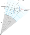Fig. 2 Geometric notations.

2.2 The refractive index model

In order to solve the system of Eqs. (13), it is necessary to provide n and dn/dh over the entire height of the atmosphere. Since the true values of the refractive index are not easily obtained, it is common to choose a particular model of the atmosphere. The choice of an appropriate theoretical model depending on the environment of the observation is very important, as it can significantly affect the refraction angle. For instance, Lovchy (2021) found differences of up to 20% on the angle of refraction at z₀ = 90° between eight different models. Even when the right simplified model is chosen, there are always substantial deviations between the modelled temperature profile and reality. Nauenberg (2017) compared the calculation of refraction using the standard profile and probe balloon measurements, and he found discrepancies of around one arcsecond for small zenith angles and even a few arcminutes from the horizon (Tables 2 and 3).

Here, we choose to follow an approximation made by several authors for the computation of the angle of refraction (Hohenkerk & Sinclair 1985; Néda & Volkan 2002; Auer & Standish 2000). Their model truncates the US76 standard atmospheric profile that is based on a piecewise linear temperature for nine atmospheric layers (COESA 1976). The choice to simplify it and reduce it to only two layers is motivated by the fact that most of the atmospheric refraction occurs in the troposphere, since the air beyond it is very sparse. This simplified model is also validated by the good match of computed results with the observational data (such as sunrise and sunset times, Néda & Volkan 2002). Earth’s atmosphere is assumed to be a perfect gas of low density in hydrostatic equilibrium. It follows the Gladstone Dale relation (Gladstone & Dale 1863): $$n-1=\kappa \rho ,$$(14)

where κ is a parameter that depends on the observation wavelength λ, and ρ is the local density of air. In order to express the density ρ as a function of altitude, it is sufficient to compute a temperature profile based on a constant temperature gradient in the troposphere: $$\omega =\text{d}T/\text{d}h=-6.5\text{K}{\text{km}}^{-1},$$(15)

and a constant temperature beyond the tropopause (i.e. the temperature gradient is nil). Setting only the value of the temperature gradient ω allows us to adapt the evolution of the temperature according to its value T₀ measured at ground level. Thus, our inputs are the temperature and pressure at ground level (respectively T₀ and P₀). The value of ω depends on the chosen model as one can see in the tables published in Anderson et al. (1986) for six reference atmospheres.

Since atmospheric refraction is only slightly sensitive to air moisture (as the values of the angle of refraction in dry and moist air are very close, van der Werf 2003), the relative humidity is considered as constant and nil in the troposphere and above it. As for the parameter κ, it is proportional to the refractivity of dry air A_d and depends on the wavelength λ. The refractivity of air is also very difficult to measure accurately, several different formulae have been proposed by different authors (Barrell et al. 1939; Edlén 1953, 1966; Owens 1967). Ciddor (1996) gave the most recent expression of refractivity in dry and moist air, also regarded as the most accurate formulae. Yet, only very few authors have compared the refraction angles for different refractivities with true experimental data. Skemer et al. (2009) used spectrography to compare atmospheric dispersion in the N band using Mathar’s model (Mathar 2007) with actual on-sky measurements; the model was in good agreement with the data. Recently, Wehbe et al. (2020) suggested a new spectrography method to measure on-sky atmospheric dispersion, showing experimentally in Wehbe et al. (2021) that, apart from the model used by Hohenkerk & Sinclair (1985), all the used models offer residual dispersions lower than 20 milliarcseconds in the 315–665nm wavelength range.

Therefore, in order to minimise the errors due to the model, we have chosen Ciddor’s and Mathar’s refractivity models and kept both the temperature and pressure at the observer as input parameters, to be as close as possible to reality. In Appendix A, we provide the details of the calculation of n and dn/dh at each altitude.

2.3 Runge-Kutta estimator of the lateral shift: b^(∞)

Now that we have chosen a model for the refractive index of Earth’s atmosphere, we next present the numerical arguments of solving the system of coupled ordinary differential Eqs. (13). This resolution provides us with a first estimator that we refer to as b^(∞)(h). The infinity exponent is related to the existence of several finite-order approximations developed in Sect. 3. In the following, we denote the values of the lateral shift obtained by evaluating the estimator b^(∞) at h = h₀ by b₀.

To solve Eqs. (13), we first notice that the db/ds variation equation also requires the value of z_∞. Therefore, it is necessary to proceed in two separate steps: we first solve a first equation system (Eqs. (13a) to (13d)) to calculate the refraction angle R_a; then, we solve the complete system (Eqs. (13a) to (13e)) to derive the lateral shift b.

Both computations are made using a fourth-order Runge-Kutta method. The first one is solved in the reverse direction of the optical propagation, while the second one is done in the direction of the optical propagation. We choose a constant integration step equal to 100m. This value is justified in Sect. 2.4.

For the first equation system (Eqs. (13a) to (13d)), we placed ourselves in the point of view of the observer and considered the following initial state: $${\left[\begin{array}{l}h\hfill \\ z\hfill \\ \theta \hfill \\ \zeta \hfill \end{array}\right]}_{h=h_0}=\left[\begin{array}{l}{h}_0\hfill \\ z_0\hfill \\ 0\hfill \\ z_0\hfill \end{array}\right].$$(16)

Then, for the second numerical equation (Eqs. (13a) to (13e)) following the ray path, we use the following initial state: $${\left[\begin{array}{l}h\hfill \\ z\hfill \\ \theta \hfill \\ \zeta \hfill \\ b\hfill \end{array}\right]}_{h=H_{\max }}=\left[\begin{array}{c}{H}_{\max }\\ z_{\infty }\\ {\theta }_{\infty }\\ {\zeta }_{\infty }\\ 0\end{array}\right],$$(17)

where the values of z_∞, θ_∞ and ζ_∞ are deduced from the previous computation, as these variables are part of the final state of the first equation system.

While we previously chose s the distance along the optical path as the integration variable, we have to define the integration limit as a function of the maximum height of Earth’s atmosphere H_max: the altitude at which the density of air can be regarded as insignificant. The value of H_max is often chosen equal to 80 km in the literature (Hohenkerk & Sinclair 1985; van der Werf 2003).

We relate the integration limit in h and s using the following approximation: $$S_{\max }=\frac{H_{\max }}{\cos z_0}.$$(18)

This expression is not appropriate close to the horizon since the refraction angle R_a grows and the approximation of 1/cos ζ in Eq. (13a) requires higher orders. However, this value of S_max is an upper bound for the effective path length of the ray in the atmosphere of thickness H_max.

We also solve each system separately in the troposphere and in the stratosphere because of the discontinuity of the refractive index derivative at the tropopause (due to the discontinuity of the temperature gradient). However, it is not straightforward to separate the two integrations when using the variable s, as we do not know where the tropopause is located in the optical path. The idea is then to modify the last integration step that straddles the two domains in such a way that it ends at the tropopause. After that, we restart the integration with the initial constant step at the tropopause.

2.4 Numerical accuracy of b^(∞)

Due to numerical integration, the accuracy of the estimator b^(∞) necessarily depends on the chosen integration step. In order to set an integration step ds, we compute the angle of refraction for several steps starting from ds = 2048 m. We chose to carry out this study in terms of the refraction angle because this is the output of the integration of the first system (Eqs. (13a) to (13d)). The integration step is divided by two at each iteration until it equals the smallest reference step chosen at ds_min = 0.5m. We choose such a small integration step in order to have a reference that is affected by the error of the numerical integration as little as possible.

The difference between the refraction angle at each ds and its value for the smallest integration step ds_min is plotted in Fig. 3: $$\text{Δ}{R}_{\text{a}}\text{/}{R}_{\text{a}}=\left|\frac{R_{\text{a}}\left(\text{d}s\right)-R_{\text{a}}\left(\text{d}{s}_{\min }\right)}{R_{\text{a}}\left(\text{d}{s}_{\min }\right)}\right|,$$(19)

and at three different zenith angles: 65°, 75°, and 85°.

We notice in Fig. 3 that the relative error decreases as the integration step ds decreases. However, the three curves often cross each other and do not decrease regularly, so some step changes have almost no effect on the value of the refraction angle. We suspect such irregularities to arise from the discontinuity of the refractive index derivative at the tropopause. We thus choose to recompute the error with a continuous profile of the refractive index derivative, using a second-order polynomial evolution of temperature near the tropopause, over 15 metres on each side. The result is shown in Fig. 4. We can see that the relative error decreases globally while oscillating around a mean slope. The relative error is smaller for larger zenith angles, which is consistent with how R_a increases with z₀ If we compare the two different models for an integration step ds = 100 m, we find that the refraction angles vary by less than 20 milliarcseconds at all zenith angles up to 85°. We therefore choose to settle for the discontinuous model. We also choose an integration step of 100 m as the relative error is smaller than 0.01%, which is, a priori, sufficient.

2.5 Values of the lateral shift

After dealing with the numerical aspects of the integration, here we study the evolution of the lateral shift using the Runge-Kutta estimator b^(∞) computed using the numerical method described in Sect. 2.3. We start by plotting in Fig. 5 the evolution of the lateral shift at ground level as a function of the apparent zenith angle. The results are computed for the standard conditions of temperature and pressure (SCTP): $$T_{\text{SCTP}}=273.15\text{K},P_{\text{SCTP}}=1000\text{hPa}.$$(20)

As a reference value for the wavelength λ₀ = 550 nm, we chose the middle of the V spectral band. We can see that the lateral shift increases with the apparent zenith angle; it tends towards 0 m when z₀ tends towards 0°, and it increases with a very steep slope near z₀ =90°, which matches perfectly with intuition and the evolution of the refraction angle R_a. The greater the zenith angle, the greater the angle of refraction and the greater the ray path through the atmosphere. We also note that the lateral shift reaches significant values beyond 20° (b ≥ 1 m), and can exceed tens of meters beyond 70°. For example, it equals 3.3 m at z₀ = 45° and is larger than 2 km at z₀ = 90°.

Fig. 3 Fig. 3. ΔRa/Ra versus the integration step.

Fig. 4 Fig. 4. ΔRa/Ra versus the integration step using a continuous derivative of the refractive index.

2.6 Influence of temperature and pressure

We now take a closer look at the distinct effects of pressure and temperature. We first deal with the pressure at the observer level, and we denote the relative difference between the lateral shift computed at a pressure P₀ and at the standard value P_SCTP = 1000 hPa by [Δb₀/b₀]^P, at T₀ = T_SCTP: $${\left[\frac{\text{Δ}{b}_0}{b_0}\right]}^{\text{P}}\left(P_0\right)=\frac{b_0\left(P_0\right)-b_0\left(P_{\text{SCTP}}\right)}{b_0\left(P_{\text{SCTP}}\right)}.$$(21)

The shift b is a priori proportional to the amount of air above the observer, as confirmed by Eq. (1) from Wallner (1976), which shows that b varies linearly with the pressure P₀ at the observer level. We can thus presume that $${\left[\frac{\text{Δ}{b}_0}{b_0}\right]}^{\text{P}}\left(P_0\right)\simeq \frac{P_0-P_{\text{SCTP}}}{P_{\text{SCTP}}}.$$(22)

This is confirmed by Fig. 6 which shows that the deviation of (Δb₀/b₀)(P₀) from its expected value (Eq. (22)) does not exceed 0.1%, even for large zenith angles. In Fig. 6, we can also see that the residual increases with the zenith angle, but it still varies slightly with pressure. Moreover, the overall lateral shift increases with the pressure since the coefficient relating the lateral shift with pressure in Eq. (1) is positive.

We next study the effect of the temperature at the observer level. From Eq. (1), we expect the effect of temperature to be negligible, and this is validated by Fig. 7, where we plot the relative difference between the lateral shift computed at a temperature T₀ and at the standard value T_SCTP = 273.15 K at P₀ = P_SCTP: $${\left[\frac{\text{Δ}{b}_0}{b_0}\right]}^{\text{T}}\left(T_0\right)=\frac{b_0\left(T_0\right)-b_0\left(T_{\text{SCTP}}\right)}{b_0\left(T_{\text{SCTP}}\right)}.$$(23)

according to the temperature at the observer level T₀ and for several apparent zenith angles. For instance, we see in Fig. 7 that the lateral shift decreases with temperature but its relative variation does not go above 1%. The greater the apparent zenith angle, the more visible the effects of temperature. We must also note that the two studied variations are in line with our expectations, since air density increases with pressure and decreases with temperature.

Fig. 5 Lateral shift at λ0 = 550 nm versus the apparent zenith angle, computed at SCTP using the estimator b(∞).

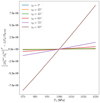Fig. 6 Deviation of [Δb0/b0]P at λ0 from ΔP0/PSCTP versus ground pressure.

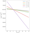Fig. 7 Variation of [Δb0/b0]T at λ0 versus ground temperature.

2.7 Dependence on observation wavelength

Since the refractive index depends on the observation wavelength λ, the effects of refraction, and, more specifically, the refraction angle and the lateral shift, also depend on λ. The angular deviation results in a chromatic blur effect (illustrated in Fig. 1) that appears when observing a celestial body, since each light ray at wavelength λ is bent by a different refraction angle R_a(λ), while the studied shift induces a lateral translation of each ray path depending on the wavelength. Both issues are more pronounced when looking towards the horizon. In this section, we study the evolution of the lateral shift as a function of wavelength.

In Fig. 8, we plot the lateral shift at h₀ = 0 as a function of wavelength and for several apparent zenith angles: $$\text{Δ}{b}_0\left(z_0,\lambda \right)=b_0\left(z_0,\lambda \right)-b_0\left(z_0,{\lambda }_0\right).$$(24)

The results are computed for the SCTP without humidity and over a range of wavelengths from 0.4 µm to 4.2 µm. Since Ciddor’s refractivity formula (Ciddor 1996) is restricted to a maximum wavelength of 1.49 µm, we covered the remaining interval using Mathar (2007) formulas. The slight jump in the curve of Fig. 8 is due to the transition between Ciddor’s and Mathar’s models at λ = 1.3 µm, while the gap between 2.5 µm and 2.9 µm results from the non-validity of Mathar’s model in this region, due to high atmospheric absorption coefficients.

We observe that the lateral shift decreases with the wavelength for any zenith angle. In order to quantify the relative extent of this decrease, in Fig. 9 we plot the relative difference in b(λ) with respect to its value at λ₀ and for a apparent zenith angles z₀ = 65°, 75°, and 85°: $$\frac{\text{Δ}{b}_0}{b_0}\left(z_0,\lambda \right)=\frac{b_0\left(z_0,\lambda \right)-b_0\left(z_0,{\lambda }_0\right)}{b_0\left(z_0,{\lambda }_0\right)}.$$(25)

We see that the variation of the lateral shift depending on the observation wavelength reaches at most 2% of its value at λ₀ in the soft UV domain. We observe that the decay slope of the lateral shift also decreases along with the wavelength, until it becomes almost horizontal in the near- and mid-infrared.

We can also notice in Fig. 9 that the curves of Δb₀/b₀ are almost identical for the three zenith angles considered. This means that the lateral shift can be approximated by a function separable into two functions of the variables λ and z₀; we see that this is indeed the case in the next section.

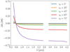Fig. 8 Absolute deviation of lateral shift from its value at λ0 = 550 nm as a function of wavelength, computed using the estimator b(∞).

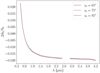Fig. 9 Relative deviation of lateral shift from its value at λ0 = 550 nm as a function of wavelength, computed using the estimator b(∞).

3 Closed-form estimators of the lateral shift

3.1 Taylor expansion of the lateral shift

The system we obtained in Sect. 2.1 does not seem to have an analytical solution, nor does it reflect the influence of the main parameters (Earth’s roundness, air density distribution, temperature and pressure at the observer) on the value of the lateral shift. In order to clarify this, we approximate the value of the lateral shift b in a way similar to Laplace’s formula for the refraction angle (Radau 1882). Laplace’s formula refers to an expression that allows the refraction angle to be calculated only from the apparent zenith angle and the weather conditions at sea level; it states that $$R_{\text{a}}\simeq {\alpha }_0\left(1-{\beta }_0\right)\tan z_0-{\alpha }_0\left({\beta }_0-\frac{{\alpha }_0}{2}\right){\tan }^3{z}_0,$$(26)

where α₀ and β₀ are defined by $${\alpha }_0=A_{\text{D}}\left(\lambda \right)\frac{P_0}{T_0},$$(27) $${\beta }_0=P_0\text{/}\left(h_0+R_{\text{T}}\right){\rho }_0,$$(28)

where P₀ and T₀ are, respectively, the temperature and pressure at the observation site, and A_D is the refractivity of dry air defined in Eq. (A.3) (α₀ still depends on the observation wavelength).

To begin with, we take advantage of the following: $$h\ll R_{\text{T}},$$(29) $$n-1\ll 1,\text{and}$$(30) $$\sin \left(z-z_{\infty }\right)\simeq z-z_{\infty }.$$(31)

The three approximations are perfectly justified since they induce a total relative error lower than 1%. First, h/R_T has as an upper bound H_max/R_pol ~ 10⁻² (where R_pol = 6356.75 km is the polar radius of Earth, and H_max is the height of the atmosphere defined in Eq. (18)). Secondly, the refractive index has its maximal value at ground level and does not exceed 10⁻³ + 1. Thirdly, the sine approximation is also valid, because the angle of refraction is always very small and does not exceed 30 arcmin (at horizon). Even when considering real weather data, as in the study carried out by Nauenberg (2017), the error resulting from the sine approximation is smaller than 0.01%.

Using the parameter α₀ defined in Eq. (27), the refractive index is written as follows: $$n=1+{\alpha }_0\frac{T_0}{P_0}\frac{P}{T}.$$(32)

Since atmospheric air is assumed to behave according to the ideal gas law, one also obtains $$n=1+{\alpha }_0\overline{\rho },$$(33)

where we denote, by ρ, the normalised density ρ/ρ₀. Knowing Eqs. (27) and (30), we have α₀ ≪ 1 as well.

In order to obtain the approximation, we start by integrating Eq. (12) between h₀ (the altitude of the observation site) and the limit of Earth’s atmosphere: $$b\left(h=h_0\right)-b\left(h\to \infty \right)={\displaystyle {\int }_{\infty }^{h_0}\sin \left(z-z_{\infty }\right)\text{d}s.}$$(34)

As depicted in Fig. 2, we choose to make the following calculations with b(h → ∞) = 0.

With the objective of using the model of the atmosphere exposed in Appendix A, we perform a change on the integration variable: $$b\left(h=h_0\right)={\displaystyle {\int }_{\infty }^{h_0}\frac{\sin \left(z-z_{\infty }\right)}{\cos \zeta }\text{d}h.}$$(35)

We also restrict ourselves to the directions of observation sufficiently above the horizon to avoid divergences.

Similarly to Laplace’s formula, we aim to express the lateral shift in terms of the moments of the atmosphere. As the lateral shift’s equation is more complex than the refraction angle equation, we define three moments: $$L^1\left(h\right)={\displaystyle {\int }_h^{\infty }\overline{\rho }\text{d}x,}$$(36a) $$L^2\left(h\right)={\displaystyle {\int }_h^{\infty }{\overline{\rho }}^2\text{d}x,}$$(36b) $$L^{\text{b}}\left(h\right)=\left[{\displaystyle {\int }_h^{\infty }x\overline{\rho }\text{d}x}\right]\text{/}{L}^1\left(h\right).$$(36c)

We define $L_0^1,L_0^2$ and $L_0^{\text{b}}$ as L¹(h₀), L²(h₀), and L^b(h₀), respectively. They are explicitly calculated in Appendix B as functions of temperature and pressure for the dry atmosphere model recalled in Appendix A. Their evolution as a function of altitude is plotted in Fig. 10.

To begin with, from Sect. 6.1.3 of Kovalevsky & Seidelmann (2004), we obtain the following approximation of z − z_∞: $$\begin{array}{lll}z\left(h\right)-z_{\infty }\hfill & =\hfill & -\text{tan}{z}_0\left({\alpha }_0\overline{\rho }-{\alpha }_0^2{\overline{\rho }}^2+{\alpha }_0^2\overline{\rho }-\frac{h{\alpha }_0\overline{\rho }}{R_{\text{T}}}-\frac{{\alpha }_0}{R_{\text{T}}}{\displaystyle {\int }_h^{\infty }\overline{\rho }}dx\right)\hfill \\ \hfill & \hfill & +{\text{tan}}^3{z}_0\left({\alpha }_{{}_0}^2{\overline{\rho }}^2/2-{\alpha }_0^2\overline{\rho }+\frac{h{\alpha }_0\overline{\rho }}{R_{\text{T}}}-\frac{{\alpha }_0}{R_{\text{T}}}{\displaystyle {\int }_h^{\infty }\overline{\rho }}dx\right).\hfill \end{array}$$(37)

Then, we expand the cosine term in Eq. (35) using Bouguer’s invariant (Eq. (3)): $$\frac{1}{\text{cos}\zeta }=\frac{1}{\sqrt{1-{\text{sin}}^2\zeta }},$$(38a) $$=\frac{\left(h+R_{\text{T}}\right)n/\left(R_{\text{T}}{n}_0\right)}{\sqrt{{\left[\left(h+R_{\text{T}}\right)n/\left(R_{\text{T}}{n}_0\right)\right]}^2-{\sin }^2{z}_0}}.$$(38b)

In addition to this, since α₀ ≪ 1 and h ≪ R_T, one obtains $$\frac{\left(h+R_{\text{T}}\right)}{R_{\text{T}}{n}_0}=\left(1+\frac{h}{R_{\text{T}}}\right)\left(\frac{1+\alpha 0\overline{\rho }}{1+{\alpha }_0}\right),$$(39a) $$=\left(1+\frac{h}{R_{\text{T}}}\right)\left(1+\alpha 0\overline{\rho }\right)\left(1-{\alpha }_0+o{\alpha }_0\right),$$(39b) $$=1+\frac{h}{R_{\text{T}}}+{\alpha }_0\left(\overline{\rho }-1\right)+o\left({\alpha }_0+\frac{h}{R_{\text{T}}}\right).$$(39c)

Based on this, we develop Eq. (38b) to the second order with respect to (h + R_T) n/R_Tn₀. We obtain $$\begin{array}{lll}\frac{1}{\text{cos}\xi }=\frac{1}{\text{cos}{z}_0}\hfill & -\hfill & \frac{{\text{tan}}^2{z}_0}{\text{cos}{z}_0}\left[\frac{\left(h+R_{\text{T}}\right)}{R_{\text{T}}{n}_0}-1\right]\hfill \\ \hfill & +\hfill & \frac{3}{2}\left[\frac{1}{{\cos }^5{z}_0}-\frac{1}{{\cos }^3{z}_0}\right]{\left[\frac{\left(h+R_{\text{T}}\right)n}{R_{\text{T}}{n}_0}-1\right]}^2.\hfill \end{array}$$(40)

As mentioned before, we note that this approximation is less accurate when the zenith angle z₀ approaches 90° (i.e. when looking close to the horizon). The reason is that 1/ cos z₀ is no longer defined when z₀ = 90°.

We then perform the product of the two approximations: Eqs. (37) and (40). This gives a second-order approximation b⁽²⁾ of the lateral shift in a dry atmosphere: $$\begin{array}{lll}{b}^{\left(2\right)}\hfill & =\hfill & \frac{\tan z_0}{\cos z_0}{\displaystyle {\int }_{h_0}^{\infty }\left({\alpha }_0\overline{\rho }-{\alpha }_0^2{\overline{\rho }}^2+{\alpha }_0^2\overline{\rho }-\frac{a_{0}h\overline{\rho }}{R_{\text{T}}}-\frac{{\alpha }_0}{R_{\text{T}}}{\displaystyle {\int }_h^{\infty }\overline{\rho }}\text{d}x\right)\text{d}h}\hfill \\ \hfill & \hfill & -\frac{{\tan }^3{z}_0}{\cos z_0}{\displaystyle {\int }_{h_0}^{\infty }\left(\frac{3}{2}{\alpha }_0^2{\overline{\rho }}^2-2{\alpha }_0^2\overline{\rho }+\frac{2a_{0}h\overline{\rho }}{R_{\text{T}}}+\frac{{\alpha }_0}{R_{\text{T}}}{\displaystyle {\int }_h^{\infty }\overline{\rho }}\text{d}x\right)\text{d}h.}\hfill \end{array}$$(41)

We can directly write most of the terms involved in Eq. (41) using the three moments of the atmosphere, except for the last term, which nests two integrals. For the latter, we perform an integration by parts: $${\displaystyle {\int }_{h_0}^{\infty }{\displaystyle {\int }_h^{\infty }\overline{\rho }\text{d}x\text{d}h}}={\displaystyle {\int }_{h_0}^{\infty }{L}^1\left(h\right)\text{d}h=-\frac{h_0{P}_0}{g{\rho }_0}+{\displaystyle {\int }_{h_0}^{\infty }h\overline{\rho }\text{d}h.}}$$(42)

Lastly, using Eq. (42), we write the lateral shift approximation using the three moments of the atmosphere. We obtain $$b^{\left(2\right)}=A_{\text{sh}}\frac{\tan z_0}{\cos z_0}-B_{\text{sh}}\frac{{\tan }^3{z}_0}{\cos z_0},$$(43)

where $$A_{\text{sh}}={\alpha }_0\left(1+\frac{h_0}{R_{\text{T}}}\right)L_0^1-2{\alpha }_0{L}_0^{\text{b}}\frac{L^1\left(h\right)}{R_{\text{T}}}-{\alpha }_0^2\left(L_0^2-L_0^1\right),$$(44) $$B_{\text{sh}}=-\frac{{\alpha }_0{h}_0}{R_{\text{T}}}{L}_0^1+3{\alpha }_0{L}_0^{\text{b}}\frac{L_0^1}{R_{\text{T}}}+{\alpha }_0^2\left(\frac{3}{2}{L}_0^2-2L_0^1\right).$$(45)

The final expression in Eq. (43) efficiently decouples the contribution of the atmosphere to the lateral shift from the contribution of the apparent zenith angle and the observation wavelength. It also spares the user having to integrate an integrand varying with the zenith angle. Thus, we have somehow established a Laplace formula for the lateral shift. Nevertheless, there is a major difference between the two formulas because of the two moments L² and L^b in the expression of b⁽²⁾. Indeed, these two lengths depend on the composition of the atmosphere and the distribution of air within it. In the following section, we describe the terms that are part of our approximation in detail.

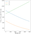Fig. 10 Evolution of the three characteristic lengths of the atmosphere as a function of the initial altitude.

3.2 First-order estimator: b⁽¹⁾

In the approximate analytic formula for the lateral shift established in Sect. 3.1, one can distinguish the first-order term that is only proportional to α₀, which we call b⁽¹⁾: $$b^{\left(1\right)}\left(h_0,z_0\right)={\alpha }_0\frac{\tan z_0}{\cos z_0}{L}_0^1.$$(46)

We thus find here Eq. (1) recalled in the introduction and which has been given in the literature by several authors. Yet, the difference between Eqs. (1) and (46) is the angle used in the tangent and cosine terms. In Eq. (1) there is a z_∞, while in Eq. (46) it is z₀. Fortunately, these two equations are equivalent because the refraction angle R_a is very small. Equation (1) has been demonstrated by Wallner under the assumption of a flat Earth, as confirmed here, since the first-order part of b⁽²⁾ tends towards b⁽¹⁾ when R_T tends towards ∞.

3.3 Second-order estimator: b⁽²⁾

Next, we take a closer look at the second-order approximation of the lateral shift Eq. (43). We can distinguish two different terms whose approximation orders are higher than the first-order: a term $b_{\text{R}}^{\left(2\right)}$ proportional to α₀/R_T, which is due to Earth’s roundness; and another term, $b_{\text{2}}^{\left(2\right)}$, proportional to ${\alpha }_{\text{0}}^2$.

We have: $$b^{\left(2\right)}=b^{\left(1\right)}+b_{\text{R}}^{\left(2\right)}+b_2^{\left(2\right)},$$(47)

where $$b_{\text{R}}^{\left(2\right)}\left(h_0\right)=\frac{{\alpha }_0}{R_{\text{T}}}\frac{\tan z_0}{{\cos }^3{z}_0}{L}_0^1\left[h_0-3L_0^b\right]+\frac{{\alpha }_0}{R_{\text{T}}}\frac{\tan z_0}{\cos z_0}{L}_0^1{L}_0^{\text{b}},$$(48a) $$b_{\text{2}}^{\left(2\right)}\left(h_0\right)={\alpha }_0^2\frac{\tan z_0}{\cos z_0}\left[L_0^1-L_0^2\right]-{\alpha }_0^2\frac{{\tan }^3{z}_0}{\cos z_0}\left[\frac{3}{2}{L}_0^2-2L_0^1\right].$$(48b)

We note that the Earth’s radius R_T does not appear in the second term $b_{\text{2}}^{\left(2\right)}$, so it is the only second-order term within the approximation of a flat Earth.

In order to capture the influence of each term, in Fig. 11 we plot the evolution in absolute values of each of the three terms according to the zenith angle. We calculated the multiplying factor α₀ at the wavelength λ₀. In Fig. 11, we observe that the main contribution comes from the flat Earth term b⁽¹⁾ and is followed by Earth’s roundness $b_R^{\left(2\right)}$, and then comes the second-order term $b_2^{\left(2\right)}$.

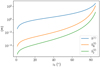Fig. 11 Evolution of the three terms in b(2) according to the zenith angle.

3.4 A separable third estimator: b^(3/2)

The dominance of the term due to Earth’s roundness $b_{\text{R}}^{\left(2\right)}$ over the term $b_{\text{2}}^{\left(2\right)}$ drives us to define a third estimator of the lateral shift denoted b^(3/2), composed of the two terms b⁽¹⁾ and $b_{\text{R}}^{\left(2\right)}$, such that $$b^{\left(3/2\right)}=b^{\left(1\right)}+b_{\text{R}}^{\left(2\right)}.$$(49)

This third approximation, between the first and second orders, has the advantage of decoupling the wavelength (only in α₀) from the zenith angle. Thanks to this, this approximation of the lateral shift is separable into functions of λ and z₀: $$b^{\left(3/2\right)}\left(h_0,z_0\right)={\alpha }_0\frac{L_0^1}{R_{\text{T}}}\frac{\tan z_0}{\cos z_0}\left\{R_{\text{T}}+L_0^{\text{b}}+\frac{1}{{\cos }^2{z}_0}\left[h_0-3L^b\left(h_0\right)\right]\right\}.$$(50)

In Fig. 12, we plot the value of $${\text{Δ}}_r{b}^{\left(3/2\right)}\left(\lambda \right)=\frac{\text{Δ}{b}^{\left(3/2\right)}\left(z_0,\lambda \right)}{b^{\left(3/2\right)}\left(z_0,{\lambda }_0\right)}=\frac{b^{\left(3/2\right)}\left(z_0,\lambda \right)-b^{\left(3/2\right)}\left(z_0,{\lambda }_0\right)}{b^{\left(3/2\right)}\left(z_0,{\lambda }_0\right)}$$(51)

as a function of λ. This quantity depends only on the wavelength λ, and is in fact simply equal to $${\text{Δ}}_r{b}^{\left(3/2\right)}\left(\lambda \right)=\frac{{\alpha }_0\left(\lambda \right)-{\alpha }_0\left({\lambda }_0\right)}{{\alpha }_0\left({\lambda }_0\right)}=\frac{n\left(\lambda \right)-n\left({\lambda }_0\right)}{n\left({\lambda }_0\right)}.$$(52)

The values of Δ_rb^(3/2) plotted in Fig. 12 are constant with respect to the zenith angle and can be directly computed with Eq. (52) using the refractivity from Eq. (A.3). Consequently, one can calculate the chromaticity of the lateral shift at any zenith angle z simply by performing the product of Δ_rb^(3/2) with the lateral shift at the chosen zenith angle and at λ₀ (b^(∞)(z, λ₀)).

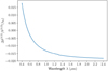Fig. 12 Chromatic behaviour of the normalised relative shift Δrb(3/2) with respect to λ0 = 550 nm using the estimator b(3/2).

3.5 Approximation error of b⁽¹⁾, b⁽²⁾, and b^(3/2) with respect to b^(∞)

In order to quantify the accuracy of the previously established approximations, we compute the values of the three estimators b⁽¹⁾, b^(3/2), and b⁽²⁾ for various zenith angles and compare them to the Runge-Kutta estimator b^(∞) (all at the SCTP) at sea level and with an observation wavelength equal to λ₀.

We plot the absolute and relative errors of the three approximations of the lateral shift, respectively, in Figs. 13 and 14: $${ϵ}_{\text{a}}^{\left(X\right)}\left(z_0\right)=\left|b^{\left(X\right)}\left(h_0=0,z_0\right)-b^{\left(\infty \right)}\left(h_0=0,z_0\right)\right|,$$(53) $${ϵ}_{\text{r}}^{\left(X\right)}\left(z_0\right)=\left|\frac{b^{\left(X\right)}\left(h_0=0,z_0\right)-b^{\left(\infty \right)}\left(h_0=0,z_0\right)}{b^{\left(\infty \right)}\left(h_0=0,z_0\right)}\right|,$$(54)

where X stands for 1, 3/2, or 2. The fluctuations observed in the curves of b⁽²⁾ in Figs. 13 and 14 are numerical and are due to the choice of the integration step for the estimator b^(∞). The chosen step (100m) allows us to make quick computations but is not small enough to ensure that the residual of the numerical integration is lower than 10⁻⁵ m.

It is clear that the three approximations deviate from the numerical solution as the zenith angle increases. This is consistent with the approximation that has been made in Eq. (40) and that is also implicitly present in Laplace’s formula and therefore in Eq. (37). From Fig. 14, we can see that the second-order approximation has a relative error of less than 1% up to a zenith angle of 75°, while the first-order approximation satisfies this requirement up to roughly 60° only. Concerning the approximation b^(3/2), it is right in between the two ‘complete’ order approximations; it suffers ten times less relative error than order 1 and thus achieves a relative error of less than 1% up to z₀ = 70°. Specifically, the b^(3/2) estimator achieves errors of less than 0.1% up to a zenith angle of 50°. We also notice on Fig. 14 that the relevance of high-order estimators is mainly found for zenith angles lower than 80°. Indeed, the relative error curves of the three estimators are very close for z₀ ≥ 80°. Finally, the choice of the appropriate estimator will depend on the tolerated error levels and the kind of application.

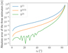Fig. 13 Absolute error of estimators b(1), b(3/2), and b(2) with respect to the Runge-Kutta estimator b(∞).

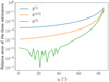Fig. 14 Relative error of the estimators b(1), b(3/2), and b(2) with respect to the Runge-Kutta estimator b(∞).

4 Applications

4.1 Wavefront sensing

This section focuses on the impact of the lateral shift in the performance of wavefront sensing systems. When dealing with atmospheric turbulence, in order to improve photometric efficiency it is usual to use different wavelengths for the science channel (the wavelength of interest for the celestial object) and the wavefront sensing channel. Yet, this scheme induces different optical paths for the related ray because of the chromaticity of the lateral shift, and hence the phase distortions seen by the two channels differ. As indicated in Wallner (1976) and Nakajima (2006), the values of the lateral shift all along the ray path at the two wavelengths (λ_SCI in the scientific channel and λ_WFS in the wavefront sensing channel) allow us to compute the wavefront phase variance associated with the chromatic shear by the use of a specific and known turbulence profile.

Our goal here is not to duplicate the mathematical developments present in the previously cited papers, but only to discuss the relevance of calculating the lateral displacement of the ray more precisely, that is using numerical computation instead of the first-order approximation.

To begin with, we assume λ_WFS = 550 nm and plot on Fig. 15 the difference between the value of the lateral shift at λ_WFS and its value at λ_SCI as a function of the observation zenith angle. Several values of λ_SCI are used; these are the central wavelengths of the spectral bands Β (445 nm), R (658 nm), I (806 nm), Η (1630nm), Κ (2190nm), L (3450nm), M (4750nm), and Ν (10500 nm). We define Δb₀ as $$\Delta b_0=b_0\left(z_0,{\lambda }_{\text{WFS}}\right)-b_0\left(z_0,{\lambda }_{\text{SCI}}\right).$$(55)

The lateral shift was purposely calculated over the entire thickness of the atmosphere, so as to simplify the computation and not consider any specific observation site. Still, this is a worst case scenario for the lateral shift as the astronomical observatories where wavefront sensing is used are located at altitudes around 3 km or above. In Fig. 15, we observe that the deviation Δb₀ increases both as functions of the zenith angle and the wavelength. The greater the difference between λ_WFS and λ_SCI, the greater Δb₀, because of the monotonic nature of the lateral shift as a function of the wavelength. We also notice the stationarity that we saw in Fig. 8, the curves of Δb₀ with a λ_SCI greater than 1630 nm are almost identical. We note that the B band is located between the R and I spectral bands due to the absolute value.

Next, we take a closer look at the effect of numerical integration. According to Eq. (10) of Nakajima (2006), the phase variance of the wavefront is proportional to (Δb₀)^5/3. In Fig. 16, we plot the ratio between Δb₀, calculated using the estimator b^(∞), and $\Delta b_{\text{0}}^{\left(1\right)}$, calculated using the first-order b⁽¹⁾, all to the power 5/3 and for λ_SCI = 1630 nm. In Fig. 16, we notice that the first-order approximation overestimates the values of the lateral displacement of the rays as the ratio is less than 1 regardless of the zenith angle. Also, the ratio studied decreases when the angle z₀ increases, but it is still very close to 1, down to 99.1% at z₀ = 50°. Given that the relative lateral deviation Δb₀ at 45° is roughly 0.1 m, the difference between the two estimators is approximately 1 mm, which is quite negligible with respect to the common Fried parameters (10 cm). The deviation is certainly higher for larger zenith angles, but those are generally avoided when correcting turbulence effects.

Based on Fig. 16, we can reasonably say that in this case, the first-order approximation is quite sufficient because there is little difference between the phase variance calculated with either the Runge-Kutta estimator or with the first-order one. Therefore, the analyses made in the literature (by Wallner 1976; Sasiela 1992; Nakajima 2006) regarding the impact of the lateral shift on adaptive optics are completely consistent, since we validate the expression of b⁽¹⁾ as a good approximation, even in the more realistic case of a spherically layered atmosphere.

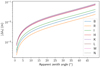Fig. 15 Difference between the lateral shift at λWFS = 550 nm and various λSCI versus zenith angle, computed using the estimator b(∞).

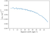Fig. 16 Ratio $\Delta b_0/\Delta b_0^{\left(1\right)}$ as a function of zenith angle.

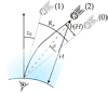Fig. 17 Difference between the apparent (1) and true (2) positions of a meteor entering Earth’s atmosphere.

4.2 Meteor trajectography

Sometimes one may want to observe objects less than 100 km away from Earth. It is the case in meteor observations with the recent creation of national and international networks of cameras dedicated to photographing meteorite falls such as the Fireball Recovery and Inter Planetary Observation Network (FRIPON (Colas et al. 2014, 2020). Usually, the goal of those projects is to estimate the landing position of the object from pictures taken at different locations by several cameras.

As mentioned in the introduction, the all-sky cameras used in meteor tracking networks rely on the astronomical catalogues to calibrate the position of objects in the sky. Thereby, the position of the object is corrected by an angle equal to the refraction angle R_a (Fig. 17), whereas the angular correction to be applied would in fact be R_a − σ, where the angle σ is shown in Fig. 17; this ‘refractive parallax’ was previously highlighted by McCrosky & Posen (1968). To illustrate, we take a look at Fig. 17, where the path of a light ray emitted by a meteorite when it enters Earth’s atmosphere is drawn. The apparent position of the meteorite corresponds to the apparent position of the faraway star (tag (1)). When this direction is corrected using the refraction angle R_a, we place the object virtually at the tag (0) and make an error equal to the shift b.

To quantify the difference between these two corrections and evaluate the error of using only the refraction angle, we can write the compensation by the lateral shift as a correction through the angle σ defined in Fig. 17 such as $$\sin \sigma =\frac{b\left(H\right)}{l\left(H\right)},$$(56)

where l(H) is the true distance between the object and the observer and H is the altitude of the object, which is assumed to be available along with the apparent zenith angle z₀.

In order to know whether this additional correction is significant or not in relation to the main refraction angle, in Fig. 18 we plot the evolution of the ratio σ/R_a according to altitude. The distance l as a function of the object’s altitude H, Earth’s radius R_T and the angle θ defined in Sect. 2.3 is given by: $$l^2=R_{\text{T}}^2+{\left(R_{\text{T}}+H\right)}^2-2R_{\text{T}}\left(R_{\text{T}}+H\right)\cos \theta .$$(57)

In order to compute the values of θ and b for an object located inside the atmosphere (at an altitude below H_max), the Runge-Kutta integration exposed in Sect. 2.3 should be made between the observer level and the altitude of the object (and no longer the atmosphere limit H_max). The angle θ is an output of the resolution of the first set of Eqs. (13a) to (13d).

Based on the reported observations of meteors (Jeanne et al. 2019; Gardiol et al. 2021; Carbognani et al. 2020), 80 km is the typical altitude at which a meteor begins to be observed, and it disappears around an altitude of 20 km as it comes apart in the atmosphere. The observation site is assumed at sea level, under the SCTP and with an observation wavelength λ₀.

We notice in Fig. 18 that the closer the object gets to Earth, the more significant the correction of angle σ becomes; it even reaches 1/3 of the refraction angle R_a at H = 20 km. Also, we can see that the ratio depends only slightly on the zenith angle for small-to-moderate angles and then increases strongly for large zenith angles (z₀ = 85°) at a given altitude. As an example of σ values, the angular error on the position of an object at an altitude of 40 km and a zenith angle of 80° (most meteors are observed at very low elevations) is equal to 1.04 arcminutes (0.2 R_a and R_a(z₀ = 80°) = 5.2 arcminutes). Moreover, if we are interested in the length deviation on the position of the object in the sky, it is simply the lateral shift induced by the bending of the ray from the object to the observer. As the object is no longer at infinity, the value of this deviation is always lower than the lateral shift integrated over the whole atmosphere, previously plotted in Fig. 5; it is therefore at worst equal to 10 m at z₀ = 60° and 70 m at z₀ = 80°.

Regarding the specifications of meteor trajectography networks, they usually use all-sky cameras that have a spatial resolution of 10 arcminutes per pixel (Gardiol et al. 2021) and do not offer the possibility of taking into account the angular correction σ. However, many networks have improved this resolution by post-processing. For instance, the CABERNET project (Egal et al. 2017) achieved a precision of 3.24 arcminutes using photographic records. Also, the fish-eye lenses of FRIPON, Jeanne et al. (2019) claim to reach an accuracy of 2 arcminutes for the positions of the stars by improving their distortion models. Compared to these two values, the additional correction σ is no less significant and should be taken into account to improve the performance of the detection systems.

A second type of (better resolved) tracking network is able to estimate the position of meteorites with errors lower than 1 arcminute, such as the CAMO network (Vida et al. 2021). These networks, which are less dense and certainly more expensive, are dedicated to the calculation of the velocity of meteors, but if scientists plan to use them to estimate the position, then the correction of the lateral shift becomes crucial.

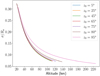Fig. 18 Correction ratio σ/Ra versus object’s altitude (H).

5 Summary and conclusion

In this work, the lateral shift in a spherical Earth approximation with a standard atmosphere model is derived for the first time, to the best of our knowledge. Values of the lateral shift are small for small zenith angles and quickly rise with a zenith angle close to 90°, as is expected from the known behaviour of the refraction angle. The shift is around 1 m at 20°, 10 m at 60°, and 2000 m at 90°. The main meteorological factor that impacts the lateral shift was found to be pressure, while the variation as a function of wavelength, which is critical for several applications, does not exceed 2% of its value at 550 nm over the visible and near-infrared spectrum. The lateral shift also depends on the altitude of the observation site. Its value calculated at an altitude of 4000 m is almost half of its value calculated at sea level.

In order to numerically compute the shift for the largest range of zenith angles, four estimators have been derived. Table 1 summarises their accuracy and corresponding equations. A source code implemented using PYTHON 3.2 is shared on the collaborative platform GitHub under the name RefractionShift² and under the open-source General Public License (3.0).

For small-to-moderate zenith angles (z₀ smaller than 55°), the simple closed-form estimator b⁽¹⁾ (previously found by Wallner 1976) can be used. This a posteriori validates the analyses and computations made for wavefront sensing based on the first-order approximation, in the regime where they are most likely to occur. For large zenith angles (down to horizon), the Runge-Kutta estimator b^(∞) offers the highest accuracy and is the one to be used for short distance astrometry, such as high-precision meteor tracking.

Lastly, for zenith angles up to 75°, a closed-form estimator b⁽²⁾ is introduced. Analogously to the well-known Laplace formula for the angle of refraction, this general-purpose estimator can further be approximated in most cases by the estimator b^(3/2), which enables a simple evaluation of the chromatic behaviour of the shift.

Acknowledgements

The work of all authors has been funded by Direction Scientifique Générale of ONERA in the framework of the COSTELLO project. The PhD work of H. Labriji is co-funded by Paris-Saclay University. We thank the reviewer for constructive criticism and valuable comments that helped to improve this paper. We also thank the language editor, N. Saint-Geniès, for corrections that helped improve this paper.

Appendix A A model for the dry atmosphere

Below, we present the derivation that leads to the expression of the optical index and its gradient, in the case of dry air and using the temperature profile presented in Section 2.2. We begin by rewriting the Gladstone-Dale relation: $$n-1=\kappa \rho .$$(A.1)

Under the ideal gas approximation, and by decoupling the dependencies in ρ and λ (respectively, density and wavelength), Eq. (A.1) reads: $$n\left(\lambda \right)-1=A_D\left(\lambda \right)\frac{P}{T},$$(A.2)

where A_D is called the reduced refractivity of dry air and is given by several models, one of the most recent expressions being given by Eq. (2) of Ciddor (1996). That is, $$\begin{array}{c}{A}_D\left(\lambda \right)={10}^{-8}[5792105{\left(238.0185-1/{\lambda }^2\right)}^{-1}+\\ 167917{\left(57.362-1/{\lambda }^2\right)}^{-1}]\frac{288.15}{1013.25}.\end{array}$$(A.3)

This expression is given for a wavelength in µm and A_D is in hPa⁻¹K. The previous expression of A_D applies for wavelengths from 300 nm to 1690 nm and is also valid over the near-infrared spectrum. We then write P/T as a function of the altitude h assuming a constant and known temperature gradient in the troposphere ω and nil temperature gradient above the tropopause. Hence, we have $$T\left(h\right)=\{\begin{array}{c}{T}_0+\omega h\text{for}\text{0}\le h\le H_t,\\ T_0+\omega H_{\text{t}}\text{otherwise}\text{.}\end{array}$$(A.4)

H_t is the altitude of the tropopause. In this framework, the pressure at a given altitude h ≤ H_t depends on the temperature as follows: $$P\left(h\right)=P_0{\left(\frac{T\left(h\right)}{T_0}\right)}^{\gamma },$$(A.5)

where $$\gamma =-\frac{g{M}_{\text{D}}}{R\omega },$$(A.6)

and

• M_D is the molar mass of dry air,

• ω: = dT/dh = − 6.5 K/km is the temperature gradient in the troposphere, and

• R is the universal gas constant.

While in the stratosphere, assuming a constant temperature, one obtains the following: $$P\left(h\right)=P_0{\left(\frac{T_t}{T_0}\right)}^{\gamma }\exp \left(-\frac{g{M}_{\text{D}}}{R{T}_t}\left(h-H_t\right)\right),$$(A.7)

where T_t is the temperature at the tropopause. We take H_t = 11 km, as in Hohenkerk & Sinclair (1985).

Hence, the refractive index with respect to height h reads $$\begin{array}{l}n\left(h,\lambda \right)-1=A_D\left(\lambda \right)P_0\hfill \\ \times \{\begin{array}{c}\frac{T{\left(h\right)}^{\gamma -1}}{T_0^{\gamma }}\text{for}\text{0}\le h\le H_t,\\ \frac{T_t^{{}^{\gamma -1}}}{T_0^{\gamma }}\exp \left(-\frac{g{M}_{\text{D}}}{R{T}_t}\left(h-H_t\right)\right)\text{for}h\ge H_t,\end{array}\hfill \end{array}$$(A.8)

and its derivative is given by $$\begin{array}{l}\frac{\text{d}n\left(h,\lambda \right)}{\text{d}h}=A_D\left(\lambda \right)P_0\hfill \\ \times \{\begin{array}{l}\omega \left(\gamma -1\right)\frac{T{\left(h\right)}^{\gamma -2}}{T_0^{\gamma }}\text{for}\text{0}\le h\le H_t,\hfill \\ -\frac{g{M}_{\text{D}}}{R{T}_t}\frac{T_t^{{}^{\gamma -1}}}{T_0^{\gamma }}\exp \left(-\frac{g{M}_{\text{D}}}{R{T}_t}\left(h-H_t\right)\right)\text{for}h\ge H_{\text{t}},\hfill \end{array}\hfill \end{array}$$(A.9)

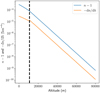Fig. A.1 Evolution of refractive index and its derivative according to altitude. The dashed line represents the altitude of the tropopause.

Figure A.1 shows the evolution of the refractive index and its derivative as a function of altitude. We notice that n and dn/dh decrease exponentially in the stratosphere (the scale of the graph on the x axis is linear and on the y axis logarithmic). Also, we observe a discontinuity of dn/dh at the boundary between the troposphere and the stratosphere, which is due to the discontinuity of the temperature gradient.

Equations (A.8) and (A.9) provide us with the evolution of the refractive index n and its derivative dn/dh in the atmosphere, under the chosen temperature and pressure model. In Sect. 2.3, these two pieces of information allow us to solve the equation system (13) and build a first numerical estimator of the lateral shift.

Appendix B The main atmospheric moments

In this paragraph, we define the main characteristic moments of the atmosphere and write them as functions of temperature and pressure using the dry model of Earth’s atmosphere. We recall the definitions of the three moments: $$L^1\left(h\right)={\displaystyle {\int }_h^{\infty }\overline{\rho }\text{d}x,}$$(B.1a) $$L^2\left(h\right)={\displaystyle {\int }_h^{\infty }{\overline{\rho }}^2\text{d}x,}$$(B.1b) $$L^{\text{b}}\left(h\right)=\left|{\displaystyle {\int }_h^{\infty }x\overline{\rho }\text{d}x}\right|/L^1\left(h\right).$$(B.1c)

L^b(h) can be interpreted as the altitude of the barycenter of an air column.

Using the hydrostatic equilibrium equation, L¹ can directly be written as $$L^{\text{1}}\left(h\right)=\frac{P\left(h\right)}{g{\rho }_0}.$$(B.2)

Besides this, using the atmosphere model exposed in Appendix A we can explicitly express the moments $L_{\text{0}}^2$ and $L_{\text{0}}^b$ as functions of T₀, H_t, and the ratio of T_t and T₀: $$r:=\frac{T_{\text{t}}}{T_0}.$$(B.3)

We obtain the following: $$L_0^2=\frac{\gamma L_0^1}{2\gamma -1}-\frac{L_0^1}{2\left(2\gamma -1\right)}{r}^{2\gamma -1}\text{and}$$(B.4) $$\begin{array}{l}{L}_0^b=h_0\left(1-\frac{r^{\gamma }}{\gamma +1}\right)+\frac{\gamma }{\gamma +1}{L}_0^1\left(1-r^{\gamma }+\frac{\gamma +1}{\gamma }{r}^{\gamma +1}\right)\hfill \\ +\frac{r^{\gamma }{H}_t}{\gamma +1}.\hfill \end{array}$$(B.5)

The evolution of L¹ L² and L^b as a function of the altitude is shown in Fig. 10. In order to obtain this figure, we changed both the altitude and the temperature and pressure values at the observation site. The evolution of P(h₀) and T(h₀) is based on the model of the dry atmosphere exposed in Appendix A using the standard values of P(h₀ = 0) and T(h₀ = 0) (Eq. (20)). Using these compact expressions of the atmospheric moments (Eqs. (B.2), (B.4) and (B.5)), we explicitly express three new estimators of the lateral shift in Sect. 3.

References

All Tables

All Figures

	Fig. 1 Bending of light rays due to atmospheric refraction.
In the text

	Fig. 2 Geometric notations.
In the text

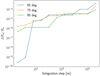	Fig. 3 Fig. 3. ΔRa/Ra versus the integration step.
In the text

	Fig. 4 Fig. 4. ΔRa/Ra versus the integration step using a continuous derivative of the refractive index.
In the text

	Fig. 5 Lateral shift at λ0 = 550 nm versus the apparent zenith angle, computed at SCTP using the estimator b(∞).
In the text

	Fig. 6 Deviation of [Δb0/b0]P at λ0 from ΔP0/PSCTP versus ground pressure.
In the text

	Fig. 7 Variation of [Δb0/b0]T at λ0 versus ground temperature.
In the text

	Fig. 8 Absolute deviation of lateral shift from its value at λ0 = 550 nm as a function of wavelength, computed using the estimator b(∞).
In the text

	Fig. 9 Relative deviation of lateral shift from its value at λ0 = 550 nm as a function of wavelength, computed using the estimator b(∞).
In the text

	Fig. 10 Evolution of the three characteristic lengths of the atmosphere as a function of the initial altitude.
In the text

	Fig. 11 Evolution of the three terms in b(2) according to the zenith angle.
In the text

	Fig. 12 Chromatic behaviour of the normalised relative shift Δrb(3/2) with respect to λ0 = 550 nm using the estimator b(3/2).
In the text

	Fig. 13 Absolute error of estimators b(1), b(3/2), and b(2) with respect to the Runge-Kutta estimator b(∞).
In the text

	Fig. 14 Relative error of the estimators b(1), b(3/2), and b(2) with respect to the Runge-Kutta estimator b(∞).
In the text

	Fig. 15 Difference between the lateral shift at λWFS = 550 nm and various λSCI versus zenith angle, computed using the estimator b(∞).
In the text

	Fig. 16 Ratio $\Delta b_0/\Delta b_0^{\left(1\right)}$ as a function of zenith angle.
In the text

	Fig. 17 Difference between the apparent (1) and true (2) positions of a meteor entering Earth’s atmosphere.
In the text

	Fig. 18 Correction ratio σ/Ra versus object’s altitude (H).
In the text

	Fig. A.1 Evolution of refractive index and its derivative according to altitude. The dashed line represents the altitude of the tropopause.
In the text

References

- Abshire, J. B., & Gardner, C. S. 1985, IEEE Transactions on Geoscience and Remote Sensing, GE-23, 414 [CrossRef] [Google Scholar]
- Anderson, G., Clough, S., Kneizys, F., Chetwynd, J., & Shettle, E. 1986, AFGL atmospheric constituent profiles (0-120 km) (Environmental Research Paper No. 964, AFGL-TR-86-0110 (Massachusetts: Air Force Geophysics Lab, Hanscom AFB, 1986) [Google Scholar]
- Aristotle. 1908, Works. Translated into English under the editorship of W.D. Ross (Oxford Clarendon Press) [Google Scholar]
- Auer, L. H., & Standish, E. M. 2000, AJ, 119, 2472 [NASA ADS] [CrossRef] [Google Scholar]
- Barrell, H., Sears, J. E. J., & Bragg, W.L. 1939, Phil. Trans. Roy. Soc. Lond. A Math. Phys. Sci., 238, 1 [CrossRef] [Google Scholar]
- Borovicka, J., Spurny, P., & Keclikova, J. 1995, A&AS, 112, 173 [Google Scholar]
- Carbognani, A., Barghini, D., Gardiol, D., et al. 2020, Eur. Phys. J. Plus, 135, 255 [Google Scholar]
- Chambers, K. 2005, in Astrometry in the Age of the Next Generation of Large Telescopes, 338, 134 [NASA ADS] [Google Scholar]
- Ciddor, P. E. 1996, Appl. Opt., 35, 1566 [Google Scholar]
- COESA 1976, U.S. Standard Atmosphere, 1976, Technical Memorandum 19770009539, NASA Technical Reports Server (NTRS) [Google Scholar]
- Colas, F., Zanda, B., Bouley, S., et al. 2014, in Proceedings of the International Meteor Conference, Giron, France, 18-21 September, 2014, 34 [Google Scholar]
- Colas, F., Zanda, B., Bouley, S., et al. 2020, A&A, 644, A53 [EDP Sciences] [Google Scholar]
- Devaney, N., Goncharov, A. V., & Dainty, J. C. 2008, Appl. Opt., 47, 1072 [NASA ADS] [CrossRef] [Google Scholar]
- Dodson, A. H. 1986, Int. J. Rem. Sens., 7, 515 [NASA ADS] [CrossRef] [Google Scholar]
- Edlén, B. 1953, JOSA, 43, 339 [CrossRef] [Google Scholar]
- Edlén, B. 1966, Metrologia, 2, 71 [CrossRef] [Google Scholar]
- Egal, A., Gural, P. S., Vaubaillon, J., Colas, F., & Thuillot, W. 2017, Icarus, 294, 43 [NASA ADS] [CrossRef] [Google Scholar]
- Gardiol, D., Barghini, D., Buzzoni, A., et al. 2021, MNRAS, 501, 1215 [Google Scholar]
- Gardner, C. S. 1977, Appl. Opt., 16, 2427 [NASA ADS] [CrossRef] [Google Scholar]
- Gladstone, J. H., & Dale, T.P. 1863, Philos. Trans. Roy. Soc. Lond., 153, 317 [NASA ADS] [CrossRef] [Google Scholar]
- Hohenkerk, C. Y., & Sinclair, A.T. 1985, The Computation of an Angular Atmospheric Refraction at Large Zenith Angles, Tech. Rep. 63, HM Nautical Almanac Office, Taunton [Google Scholar]
- Jeanne, S., Colas, F., Zanda, B., et al. 2019, A&A, 627, A78 [EDP Sciences] [Google Scholar]
- Jolissaint, L., & Kendrew, S. 2010, in 1st AO4ELT conference - Adaptive Optics for Extremely Large Telescopes, Paris, France, 05021 [CrossRef] [Google Scholar]
- Kovalevsky, J., & Seidelmann, P. K. 2004, Fundamentals of Astrometry (Cambridge: Cambridge University Press) [CrossRef] [Google Scholar]
- Kristensen, L. K. 1998, Astron. Nachr., 319, 193 [NASA ADS] [CrossRef] [Google Scholar]
- Li, S., Zhang, G., Tang, X., & Huang, W. 2016, Rem. Sens. Lett., 7, 985 [CrossRef] [Google Scholar]
- Lovchy, I. L. 2021, J. Opt. Technol., 88, 60 [CrossRef] [Google Scholar]
- Mahan, A. I. 1962, Appl. Opt., 1, 497 [NASA ADS] [CrossRef] [Google Scholar]
- Marini, J. W. 1972, Radio Sci., 7, 223 [NASA ADS] [CrossRef] [Google Scholar]
- Mathar, R. J. 2007, J. Opt. A: Pure Appl. Opt., 9, 470 [NASA ADS] [CrossRef] [Google Scholar]
- McCrosky, R. E., & Posen, A. 1968, SAO Special Report, 273 [Google Scholar]
- Nakajima, T. 2006, ApJ, 652, 1782 [NASA ADS] [CrossRef] [Google Scholar]
- Nauenberg, M. 2017, PASP, 129, 044503 [NASA ADS] [CrossRef] [Google Scholar]
- Néda, Z., & Volkan, S. 2002, Am. J. Phys., 71 [Google Scholar]
- Owens, J. C. 1967, Appl. Opt., 6, 51 [NASA ADS] [CrossRef] [Google Scholar]
- Owner-Petersen, M. 2006, in Advances in Adaptive Optics II, 6272, 62722F [NASA ADS] [CrossRef] [Google Scholar]
- Owner-Petersen, M., & Goncharov, A. 2004, Ground-based Telescopes, Proc. SPIE, 5489 [Google Scholar]
- Pannetier, C., Mourard, D., Cassaing, F., et al. 2021, MNRAS, 507, 1369 [NASA ADS] [CrossRef] [Google Scholar]
- Radau, R. 1882, Annales de l’Observatoire de Paris, B.1 [Google Scholar]
- Regiomontanus, J. 1544, Scripta de Torqueto, Astrolabio armillari, Regula magna Ptolemaica … aucta necessariis, Joannis Schoneri Carolostadii additionibus … Item, Libellus M. Georgii Purbachii de Quadrato Geometrico (Jo. Montanus) [Google Scholar]
- Saastamoinen, J. 1972, Bull. Géodésique, 105, 279 [Google Scholar]
- Sasiela, R. J. 1992, J. Opt. Soc. Am., 9, 1398 [NASA ADS] [CrossRef] [Google Scholar]
- Schmid, H. 1963, The Influence of Atmospheric Refraction on Directions Measured to and from a Satellite, GIMRADA Research note (Army Engineer Geodesy, Intelligence and Mapping Research and Development Agency) [CrossRef] [Google Scholar]
- Seidelmann, P. K., ed. 1992, Explanatory Supplement to the Astronomical Almanac (University Science Books), section: 3.28 Refraction [Google Scholar]
- Skemer, A. J., Hinz, P.M., Hoffmann, W.F., et al. 2009, PASP, 121, 897 [NASA ADS] [CrossRef] [Google Scholar]
- Stone, R. C. 1996, PASP, 108, 1051 [NASA ADS] [CrossRef] [Google Scholar]
- Thomas, M. E., & Joseph, R. I. 1996, Johns Hopkins APL Tech. Digest, 17, 279 [NASA ADS] [Google Scholar]
- Tóth, J., Kornoš, L., Zigo, P., et al. 2015, Planet. Space Sci., 118, 102 [CrossRef] [Google Scholar]
- van den Born, J.A., & Jellema, W. 2020, MNRAS, 496, 4266 [NASA ADS] [CrossRef] [Google Scholar]
- van der Werf, S.Y. 2003, Appl. Opt., 42, 354 [NASA ADS] [CrossRef] [Google Scholar]
- van der Werf, S.Y. 2008, Appl. Opt., 47, 153 [NASA ADS] [CrossRef] [Google Scholar]
- Vida, D., Brown, P. G., Campbell-Brown, M., et al. 2021, Icarus, 354, 114097 [CrossRef] [Google Scholar]
- Wallner, E. P. 1976, in Imaging Through the Atmosphere, 0075, 119 [NASA ADS] [CrossRef] [Google Scholar]
- Wallner, E. P. 1977, JOSA, 67, 407 [NASA ADS] [CrossRef] [Google Scholar]
- Wehbe, B., Cabral, A., & Avila, G. 2020, MNRAS, 499, 183 [NASA ADS] [CrossRef] [Google Scholar]
- Wehbe, B., Cabral, A., Sbordone, L., & Avila, G. 2021, MNRAS, 503, 3818 [NASA ADS] [CrossRef] [Google Scholar]
- Wittmann, A. D. 1997, Astron. Nachr., 318, 305 [NASA ADS] [CrossRef] [Google Scholar]
- Yan, M., Wang, C., Ma, J., Wang, Z., & Yu, B. 2016, Photogr. Eng. Rem. Sens., 82, 427 [CrossRef] [Google Scholar]
Labriji, H., https://github.com/OneraHub/RefractionShift
See footnote 1.