| Issue |
A&A
Volume 662, June 2022
|
|
|---|---|---|
| Article Number | A2 | |
| Number of page(s) | 15 | |
| Section | Planets and planetary systems | |
| DOI | https://doi.org/10.1051/0004-6361/202141296 | |
| Published online | 25 May 2022 | |
Discrete Element Modeling of Aeolian-like Morphologies on Comet 67P/Churyumov-Gerasimenko
1
Institute of Planetary Research, German Aerospace Center (DLR),
Rutherfordstr. 2,
12489
Berlin,
Germany
e-mail: This email address is being protected from spambots. You need JavaScript enabled to view it.
2
Institute of Physics and Astronomy, University of Potsdam,
Potsdam,
Germany
Received:
12
May
2021
Accepted:
13
August
2021
Abstract
Context. Even after the Rosetta mission, some of the mechanical parameters of comet 67P/Churyumov-Gerasimenko’s surface material are still not well constrained. They are needed to improve our understanding of cometary activity or for planning sample return procedures.
Aims. We discuss the physical process dominating the formation of aeolian-like surface features in the form of moats and wind taillike bedforms around obstacles and investigate the mechanical and geometrical parameters involved.
Methods. By applying the discrete element method (DEM) in a low-gravity environment, we numerically simulated the dynamics of the surface layer particles and the particle stream involved in the formation of aeolian-like morphological features. The material is composed of polydisperse spherical particles that consist of a mixture of dust and water ice, with interparticle forces given by the Hertz contact model, cohesion, friction, and rolling friction. We determined a working set of parameters that enables simulations to be reasonably realistic and investigated morphological changes when modifying these parameters.
Results. The aeolian-like surface features are reasonably well reproduced using model materials with a tensile strength on the order of 0.1–1 Pa. Stronger materials and obstacles with round shapes impede the formation of a moat and a wind tail. The integrated dust flux required for the formation of moats and wind tails is on the order of 100 kg m−2, which, based on the timescale of morphological changes inferred from Rosetta images, translates to a near-surface particle density on the order of 10−6–10−4 kgm−3.
Conclusions. DEM modeling of the aeolian-like surface features reveals complex formation mechanisms that involve both deposition of ejected material and surface erosion. More numerical work and additional in situ measurements or sample return missions are needed to better investigate mechanical parameters of cometary surface material and to understand the mechanics of cometary activity.
Key words: comets: general / comets: individual: 67P/Churyumov-Gerasimenko / methods: numerical
© ESO 2022
1 Introduction
The visit of the Rosetta spacecraft at comet 67P/Churyumov-Gerasimenko (hereafter 67P) revealed a previously unknown diversity of geomorphologic surface features and landforms on a comet (Thomas et al. 2015c; El-Maarry et al. 2019). These features are influenced by the physical material properties and environment in which they form and they have been used to constrain physical parameters of the cometary regolith (Attree et al. 2018; Biele et al. 2015).
One of the most surprising morphologic observations on 67P is the presence of aeolian-like bedforms (e.g., Mottola et al. 2015; Thomas et al. 2015a,c) identified in high-resolution image data of the ROLIS descent imager (Mottola et al. 2007) onboard the Philae lander and the OSIRIS orbiter camera (Keller et al. 2007) onboard the Rosetta spacecraft. These bedforms involve ripple-like structures in the Hapi region (the “neck” of the comet) (Thomas et al. 2015c) as well as elongated deposits of granular material and semicircular depressions around several larger boulders (>5 m) resembling wind tails and moats as known from planets with atmospheres (Fig. 1). These features commonly form by the accumulation or erosion of granular media such as sand by wind. Examples of wind tails and moats have been observed on Earth and Mars (e.g., Greeley et al. 1999, 2002; Golombek et al. 2006) (Fig. 2) and are usually associated with turbulences. However, turbulences do not occur on an almost atmosphereless comet, and the features are certainly of different origin. Nevertheless, the existence of these bedforms indicates that aeolian-like processes can transport particles across the surface of the nucleus and become manifest where they interact with obstacles such as boulders.
Previous studies have been aimed at finding an answer to the question of how to explain aeolian-like granular transport on a planetary body with an extremely rarefied exosphere and with an almost negligible gravitation, hence, without some of the fundamental physical mechanisms generally responsible for particle motion (Thomas et al. 2015b). Several studies have suggested that they form as a result of abrasion of a sand bed induced by air fall particles (Kramer & Noack 2015; Mottola et al. 2015; Thomas et al. 2015a).
In this paper, we concentrate on the identification of the physical processes dominating the formation of moats and wind tail-like bedforms around obstacles and investigate mechanical and geometrical parameters involved. Due to the similarity in morphology to the well-known bedforms on Mars and Earth, we use the term “wind tails” for the elongated bedforms associated with obstacles. However, we do not intend to imply that wind is involved in the formation of these features on the nucleus.
To complement the available measurements, improve our understanding of the dynamic processes involved in forming wind tails and moats, and constrain the physical parameter space of the materials involved, we applied numerical simulations. These can be used to constrain some of the micro- and macro-mechanical parameters, for example, by excluding certain parameter ranges or combinations incompatible with the development of the observed morphological features. The DEM is a widely accepted method for modeling granular and discontinuous materials. It is well suited to describe the separate, discrete particles presumably involved in the formation of the moat and wind tail structures. The present study continues previous work (Kappel et al. 2020), where we applied the DEM method to investigate the morphologies of boulders and cliffs observed on 67P.
Section 2 shows the distribution of moats and wind tails on comet 67P as well as more detailed measurements for two selected boulders. Section 3.1 gives an overview of our numerical DEM modeling of these features. The investigated simulation scenario is introduced in Sect. 3.2, and the simulation outcomes and changes when varying its setup are presented and discussed in Sect. 4. Finally, conclusions and an outlook are given in Sect. 5.
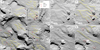 |
Fig. 1 Mapping of aeolian-like morphologies on OSIRIS image data at the Agilkia touchdown 1 site, as an example for the 362 images analyzed. The orientation of the moats, wind tails, and smooth ridges indicate material transport from the same source direction, i.e., from the lower right to the upper left of this image (OSIRIS image NAC_2014-11-12T15.43.51.584Z; image credit: MPS/UPD/LAM/IAA/SSO/INTA/UPM/DASP/IDA). |
2 Bedform description and distribution
Using preperihelion OSIRIS images with resolutions of 50 cm/pixel or better, we identified boulders with aeolian-taillike morphologies globally. Although we examined the entire illuminated surface of 67P, we focused on areas with air fall deposits given their association of aeolian-like features. In total, we examined 362 images taken between October 2014 and February 2015 of which 41 were used to take measurements of boulders and wind tails.
The majority of the wind tails on comet 67P is located on the small lobe of the nucleus in the Ma’at region (see El-Maarry et al. (2015) for regional boundaries and nomenclature), whereas other areas are depleted in this respect (Fig. 3). All wind tails occur in regions covered with air fall deposits. The average boulder size (measured as the mean of length and width of a boulder along and perpendicular to the wind tail direction) is 15.9 m ± 6.7m (one standard deviation) with a minimum of 4.6 m (possibly biased due to the spatial resolution limit) and a maximum of 35.5 m. The average length of the wind tails is around 15.2m ± 9.9m with a minimum of 4.9 m and a maximum of 73.6 m, reflecting the variable size of boulders on the nucleus. Most wind tails are shorter than 30 m, and the lower limit of measured wind tail length as well as boulder size depends largely on the image resolution. Boulder height and wind tail length are moderately correlated (Fig. 4) with a Pearson correlation coefficient of 0.52. A linear fit to the data has a slope of 0.94, which – assuming the wind tail is simply the geometrically shielded region behind the boulder – corresponds to an incident angle of the particle wind of about 45°.
We measured the heights of two wind tails at Philae’s first touchdown site in the Agilkia region in a digital terrain model (L. Jorda, personal comm.), which was generated from OSIRIS images using the method described by Jorda et al. (2016). One of those wind tails is associated with the ~5-m-sized boulder located right at the first touchdown site, and the other one is at a ~13-m-sized boulder about 60 m northwest of the first boulder (Figs. 5a,b). The maximum wind tail elevations range between 0.5 m and about 3 m depending on the boulder and the location of the cross section relative to the wind tail (Figs. 5c–f). Typically, the height of a wind tail on 67P reaches one third of the boulder’s height. It is noteworthy that the size of the wind tails in relation to their obstacles on 67P is much larger than those known from Earth and Mars (Golombek et al. 2006).
The moat at the 5-m-sized boulder spans up to 2 m at its widest extent and has a maximum depth of about 40 cm (cf. Fig. 2c and longitudinal profile in Fig. 5d). It is difficult to estimate how many boulders on the comet’s surface exhibiting a wind tail are also associated with a moat, since identification of the latter strongly depends on image resolution. Our survey can only provide a conservative estimate on the order of 20%, representing 14 boulders with moats identified out of a total of 65 boulders with wind tails. However, due to the observation bias and due to the fact that many moats might be hard to discern because they are optically occluded by the boulders, it is plausible to assume that the actual number of moats is substantially higher.
Tirsch et al. (2017b,a) noted a clear correlation of wind tail orientation in a given vicinity indicating a common source of the transport process. For instance, the preferred orientation of the wind tails in the Ma’at region is to the north (Fig. 3). Wind tails located in other parts of the comet mostly have a different orientation than to the north indicating different source regions of the air fall stream. The clustering of wind tails in the Ma’at region is consistent with the findings of Kramer & Noack (2015) based on global gas and dust dynamics simulations and Lai et al. (2016) suggesting erosion of particles in Ma’at and Ash. In addition, the orientation of the wind tails agrees with the seasonal particle transport from south to north as suggested by Keller et al. (2017).
Variations in the covering of boulders with air fall particles indicate a dynamic formation process. However, the temporal evolution of these features could not be directly observed and probably takes place on scales below the image resolution.
Mottola et al. (2015) modeled the formation of wind tails using a simple, three-dimensional cellular automaton model that allowed air fall particles to erode a preexisting particle bed around a buried boulder. Although this model does not take into consideration particle deposition and redistribution, it successfully explains the morphologic formation of wind tails and moats as a purely erosive process. However, this model may be oversimplified and physical parameters related to the particle bed and boulder could not be derived. Additionally, Davidsson et al. (2020) suggested a net accumulation of air fall material in this region of up to 3.6 m based on a numerical model including orbit dynamics, thermophysics of the nucleus, and hydrodynamics of the gas flow. In the following, we complement our measurements of wind tails and moats on 67P with new improved numerical simulations including both particle deposition and erosion.
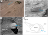 |
Fig. 2 Wind tails and moats on different planetary bodies. (a) Wind tails associated with vegetation acting as obstacles at Grand Falls Dune Field, Arizona, USA (Photo: D. Tirsch). (b) Boulder “Barnacle Bill” at the Mars Path Finder landing site. This 43-by-22-cm-sized rock is associated with a distinctive moat to its right and a wind tail to its left (subset of MPF image 81008 with parts of the Sojourner rover at the lower right). (c) 5-m-sized boulder at Philae’s first touchdown site “Agilkia” on comet 67P. White dashed lines trace the shape of the moat and the wind tail associated with this boulder (subset of ROLIS image ROL_FS3_141112153316_336_02). (d) Sketch showing the typical shape of a moat and a wind tail associated with an obstacle. Blue arrows indicate the wind direction in panels a, b, and d as well as the transport direction of air fall particles in panel c. |
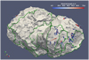 |
Fig. 3 Distribution of boulders (red spheres) with wind tails (arrows) on 67P projected onto a digital shape model by Preusker et al. (2017) with 67P’s morphologic regions outlined (El-Maarry et al. 2015). The arrows’ directions represent wind tail orientation including inclination and thus illustrate the presumed directions of the incoming particle streams, and their colors indicate the wind tail lengths. The boulder sizes are matched by the red sphere sizes. Most of these features are found in the Ma’at and Serqet regions, which are located at “the top of the head”, i.e., the northern part of the small lobe (Otto et al. 2017). |
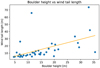 |
Fig. 4 Scatter plot of boulder height and wind tail length. The orange line is a linear fit with a slope of 0.94. |
3 Numerical Simulations
3.1 Discrete Element Modeling
The dynamics of the granular cometary surface material is modeled with the open source DEM simulation code LIGGGHTS (Kloss et al. 2012). Generally, we assume the particles to be represented by polydisperse spheres consisting of a mixture of dust and water ice, in contrast to Kappel et al. (2020), where the material consisted of a mixture of particles consisting either of dust or of ice. The spheres interact according to the Hertz contact model (Hertz 1882) and additionally are subject to cohesion from unsintered contacts, translational friction, rolling friction (Ai et al. 2011), and ambient surface acceleration. Furthermore, parallel bonds (Potyondy & Cundall 2004) between the spheres can be introduced that break when the interparticle stresses exceed certain threshold values. This way, we can also model the hard consolidated terrain that was found at many places on the surface of 67P and may result from water ice sintering (Spohn et al. 2015). However, this aspect is not considered in the present work, which causes the ice to differ from the dust only by its solid mass density and limits the influence of the ice on the results: When the bulk material’s mass density is fixed to that of 67P, the ice’s lower solid mass density leads to a less porous, slightly stronger bulk material (calculations provided in Sect. 3.2). To enable the simulation of macroscopic scenarios with relatively small particles, we apply the coarse-graining technique (Bierwisch et al. 2009). A detailed description of each of these aspects has been provided with our first application of this model in Kappel et al. (2020). Since then no fundamental changes to the model have been applied, but in the present work we use a partly different set of model parameters, which are given and whose choice is motivated in Sect. 3.2.
3.2 Simulation Scenario
To model the scenario of wind tail and moat formation, we introduce a steady stream of particles colliding with a large obstacle in a particle bed. The incoming particles are set to move at a certain velocity on inclined, unidirectional trajectories. In the following, by the use of the words “in front of” (“behind”) we refer to the area facing (shadowed from) the particle stream as seen from the obstacle. To avoid boundary effects, the simulation geometry is set to be periodic in the horizontal dimensions.
The simulation is composed of two main parts – first the construction of a particle bed and the placement of an obstacle in the center of it, and then the insertion of a particle wind from above the obstacle. It starts by loosely filling a horizontal layer at the bottom of a cuboid simulation domain with non-contacting randomly positioned and sized (chosen from eight discrete sizes) spherical particles. Particles from a region in the center of the particle cloud are removed and replaced by an obstacle made up of wall elements or of a primitive sphere. The particle cloud is then compacted to the desired level by uniformly accelerating all particles to the same given downward velocity. As the particles fall down, they collide with each other or a wall at the bottom and dissipate their kinetic energy. By changing the given downward velocity and (temporarily) the interparticle contact parameters, we can control the bulk mass density and porosity of the emerging particle layer. After settling, the upper excess particles beyond the given layer thickness are removed and the simulation continued until relaxation. Then a stream of particles (“wind”) with a given mass rate and downward velocity (inclination 45°) is continuously inserted in a horizontal layer above the obstacle. When impacting the obstacle or the particle bed, the wind particles can either get scattered or absorbed and cause the ejection of secondary particles, all together forming a particle cloud (“atmosphere”) above the particle bed. Since the deeper particles in the bed are also stirred, it sometimes becomes challenging to define which of the particles still belong to the bed and which to the atmosphere. The simulation is run until a steady atmosphere is established and no further morphological changes of the surface are observed (apart from changes of the overall level). An example of this scenario is shown in Fig. 6. The definition of the coordinate axes (x, y, z) is as seen in this figure, where z increases with increasing altitude counting from the initial surface level right before the onset of the particle wind as level zero.
Due to the limited available computational resources, the simulations have to be restricted to a finite portion of the nucleus surface. Our particle bed measures 13.5 m × 9m in the horizontal dimensions to significantly exceed our obstacle size (order of 3 m) and give room for the dynamics that dominate in the direction of particle insertion. In contrast, the vertical direction is only bounded by a wall at the bottom of the particle bed and is always expanded upwards to the particle with the currently highest altitude. The obstacle in the center of the particle bed is either a half-sphere, an upright cylinder, or a cube, whereas the cube can be rotated around its vertical axis to change its alignment with the particle wind. The rotation angle is set to 30°, which allows us to investigate the effect of two different front face alignments in a single simulation. The edge length of the cube and the diameter and height of the cylinder are 2.1 m, while the sphere is larger having a diameter of 2.7 m. Since the obstacles’ lower parts are buried in the particle bed, the initial height of the cube and cylinder and that of the sphere above the surrounding particle bed level is only 1.5 m and 1 m, respectively, and slowly decreases as the surface level rises due to the insertion of additional particles.
Our particles are polydisperse spheres that each consist of a mixture of dust and water ice. They are assumed to resemble fluffy aggregates (motivated by the appearance of the particle beds in OSIRIS images and MIDAS measurements of coma particles, Mannel et al. 2019, that may present a source of our studied particle beds) that, in addition to the porosity of the particle bed 1 − ϕ1, also have an internal porosity 1 − ϕ2. For simplicity, we assume that both filling factors are the same, that is ϕ = ϕ1 = ϕ2. Then the mass density of the bulk material is given by ϕ2ρ, where ρ = (1 − x) ρdust + xρice is the mixing density of the solid material for an ice volume fraction x and solid mass densities ρdust = 2000 kg m−3 and ρice = 920 kg m−3 for the dust and the water ice particles, respectively. For a mixture with a dust-to-ice solid volume ratio of 2:1 (Pätzold et al. 2016), this mixing density is 1640 kg m−3. With this, the filling factor results in 57% (corresponding to a bulk density of the aggregates of 940 kg m−3) in order to achieve an overall bulk density that is similar to the global mean value of 538 kg m−3 of comet 67P (Preusker et al. 2017).
To avoid a degeneration of the size-dependent contact forces, we use a discrete particle size distribution with eight different equally spaced radii (R = 3−6 cm). The cumulative distribution is set to follow a power-law with index ic such that the number of particles with radius larger than R is proportional to  . Mottola et al. (2015) reported ROLIS measurements for the Agilkia region on 67P, the initial touchdown site of Rosetta’s Philae lander, exhibiting values of ic in the range from 2.2 to 3.5. In our simulations, we use ic = 2.5, and the ratio between the largest and the smallest particle radius is 2, meaning that eight of the smallest particles have the same mass as one of the largest ones. The mechanical parameters of the particles are largely adopted from our previous work regarding the stability of boulders and cliffs on 67P (Kappel et al. 2020), with some necessary changes to account for the particles resembling fluffy aggregates in this work. As default we set Poisson’s ratio of both the particles and the obstacle to v = 0.3. The three friction coefficients (sliding and rolling friction coefficients μ and μr, rolling viscous damping ratio ηr) are all set to 1.0, which has led to realistic morphologies in our boulder and cliff simulations (Kappel et al. 2020). Young’s modulus and the coefficient of restitution are set to lower values than in the cited paper, that is Y = 105 Pa and er = 0.2 instead of Y = 108 Pa and er = 0.3, respectively, in both cases reflecting the more deformable and dissipative nature of our fluffy particles and that our particles collide with higher speeds on the order of 1 ms−1 instead of 0.1m s−1, compare Brilliantov et al. (1996). For the calculation of the cohesion, we use the Derjaguin-Muller-Toporov model (DMT) (Muller et al. 1983), where the cohesive force is given by Fc = −2πR*ω, with the effective radius
  of two contacting particles with radii R1 and R2 and the surface energy density ω. We take, in our notation, ω = 0.028 J m−2 determined by pull-off force measurements of micron-sized silica spheres by Heim et al. (1999). Deviations from this reference set of parameters, for example, when discussing the influence of these parameters, are mentioned separately.
The incoming particles are likely to have a velocity vins on the order but somewhat slower than the orbital velocity, because much faster particles are not bound by 67P’s gravity and therefore less likely contribute to our steady model particle stream, and much slower ones have a too short trajectory length to be compatible with an emission in a well separated source region, such as the southern hemisphere in the frame of the seasonal global mass transfer discussed by Keller et al. (2017). We do not regard slow particles mobilized by impacting other particles as a driver of the wind tail and moat formation but already as a secondary effect that we aim to self-consistently reproduce with our model. For a rough estimate of vins, we neglect the complex dust dynamics near the comet and instead assume the particles to be solely governed by the gravity of a spherical body with the same mass (9.982 × 10¹² kg) and bulk density (538 kg m−3, both Preusker et al. 2017) as 67P. Such a body has an equivalent radius of R = 1640 m and a surface acceleration of g = 2.4 × 10⁻⁴ m s−2 (neglecting the centrifugal force due to the rotation of the comet), which gives a speed of  for a circular orbit close to the surface. Therefore the speed of the wind particles is set to a somewhat lower value of vins = 0.5 ms−1, where the exact choice is not so important for the simulation. In our simulations, we use a typical surface acceleration of 1.8 × 10⁻⁴m s−2 calculated as the median over all facets of the 67P shape model (Preusker et al. 2017) taking into account the centrifugal force. Regarding the flux density of the incoming particles, we need to set a model value that, on the one hand, exceeds a certain lower limit in order to see erosional and depositional effects at all within a reasonable simulation time, and, on the other hand, should not be too large to avoid excessive shielding of the incoming particles by the developing atmosphere. We use a value of fins = 2.5 × 10⁻³ kg m−2 s−1 (measured perpendicular to the surface normal), which was found to cause atmospheric collisions for less than 5% of the incoming particles. The actual value on 67P will be estimated later and is much smaller than that, but as long as the stated conditions are met, the effect on the morphologic development should be sufficiently linear to scale the elapsed simulation time with regard to the incoming flux density.
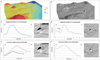 |
Fig. 5 Morphometry of wind tails at the Agilkia landing site. (a and b): perspective views showing the two boulders based on OSIRIS images and DTM data (Jorda et al. 2016). Colors in a encode elevations from – 16 m (blue) to + 15 m (red). Labels in b indicate boulder sizes. The lateral and vertical DTM resolutions are about 35 and 10 cm per pixel, respectively. (c–f): longitudinal and transverse cross sections of the wind tails (and the moat) associated with the two boulders at Agilkia (Tirsch et al. 2017a). The size of the wind tail in profile (ƒ) is at the limit of the DTM resolution which is the reason for the step-like shape of the profile. |
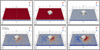 |
Fig. 6 Construction of an obstacle in the center of a cometary particle bed made up of 140 000 polydisperse spheres consisting of a porous dust-ice mixture with a volume ratio of 2:1, and exposure to a particle wind. Top row: construction of the particle bed. (a) Loose filling of a horizontal layer at the bottom of the simulation domain with non-contacting randomly positioned and sized (chosen from eight discrete sizes) spherical particles. (b) Removal of particles in the center region and insertion of an obstacle built of wall elements. (c) Compaction of the particle layer to the bulk mass density and porosity of comet 67P and removal of particles above the given layer thickness. Bottom row: (d–f) several stages after the introduction of the particle wind. Particles from the granular atmosphere are removed for better representation. The color bar is adapted to the changing overall level of the particle bed. |
4 Results and discussion
In this section, we report the outcomes of our simulations for the wind tail scenario and the changes when modifying the setup or varying the parameters. We obtain a slowly rising particle equilibrium surface resulting from the local balance between erosion by impacting fast particles and deposition of mobilized slow particles. This re-distribution of surface material is the key difference to the simpler model of Mottola et al. (2015), which only includes erosion from the initial impact but not the deposition of created ejecta. In our model the obstacle partly shields the area behind it from erosion, which results in the formation of a “wind tail”, where deposition predominates erosion. In front of the obstacle, additional erosion by incoming particles reflected at the obstacle can yield a moat. This depends on the shape of the obstacle, the flat front face of a cube being more effective in eroding a localized area than the rounded shapes of cylinders or spheres that distribute the reflected particles into many directions. Particle sizes, interparticle forces as well as velocity and inclination of the incoming particles affect the morphology of these surface features, which enables us to constrain some of these parameters by comparing simulation results to observations.
Avoiding boundary effects
First we start without periodicity in the horizontal dimensions. The simulation domain is arranged so that the obstacle is roughly in the center. The incoming particle stream is inserted starting from just above the highest point of the obstacle (to minimize interferences with the developing atmosphere), and such that it covers the entire particle bed (also after parts of it have been eroded). The insertion height has to account for the inclination of the incoming particle stream, that is a sufficient horizontal extent of the source region or a corresponding lateral shift with respect to the particle bed counteracting the offset between the positions of the particle insertion and the particle interaction with the surface. We choose an orientation where the stream is coming from the left (with respect to the representation of the simulations in the figures). However, we found this setup to lead to boundary effects: the erosion of the particle bed is most pronounced at its leftmost part. Furthermore, particles approaching the other three horizontal sides are affected as well when either they can leave the domain (and are deleted) or when a (high or low) wall keeps them from leaving. One option to avoid such boundary effects in a given region around the obstacle would be to use a simulation domain with boundaries horizontally farther away from the obstacle, but this is numerically inefficient, and after a certain elapsed time, the boundary effects will have reached this region even then. We choose another option where particles leaving the domain on one side are re-introduced in the domain from exactly the opposite side with the same velocity vector. In other words, we use a periodic geometry in the horizontal dimensions. In this case, the particle stream is injected from a region that horizontally extends exactly over the particle bed, and there is no need to shift this source region to the left because of the inclination as described above. Consequently, the simulation setup is equivalent to a domain with infinite horizontal extent and infinitely many periodically placed obstacles, with a horizontally infinitely extended source region of the particle stream. This way, no boundary effects can develop, but we have to ensure that the vertical boundaries of the basic domain are reasonably far away from the basic obstacle such that the distances between obstacles in the periodic geometry suffice to keep interferences between them low. This setup has the side effect that the number of particles in the basic domain continually increases, raising the level of the particle bed and slowing down the simulation with time. The flux density of the incoming particles is constant throughout the simulation.
Formation of dust atmosphere
An interesting effect we could observe is the formation of an atmosphere-like particle assembly above the surface. We use the term “atmosphere” for it, because of the obvious analogy to the usual gas molecule atmosphere. This granular atmosphere is caused by particles originating from the surface that have been mobilized by the impinging particle stream. Here we exclude the incoming particle stream itself (the “wind”) that has a different dynamical character as well as the static or nearly static surface particles.
At any given time only a few wind particles are on their incoming ballistic trajectories before impacting the surface or colliding with atmospheric particles. Once they hit the surface, they typically cause one or more surface particles to be ejected, mostly at slower speed than that of the wind stream, but this depends on the collision geometry, relative particle sizes, and interparticle forces. The ejected particles and the deflected injected ones become new members of the atmosphere and move on ballistic curves until they collide with other particles, either on the surface, thereby possibly mobilizing further surface particles, or in the atmosphere. The slowest particles settle and are finally deposited on the surface, thereby leaving the atmosphere and raising the surface level. This way, energy and momentum of the wind are not only dissipated into the surface layer but are also distributed into the atmosphere, into translational and rotational degrees of freedom. Until a stationary equilibrium is achieved, the density of the atmosphere increases with time.
The atmosphere exhibits a slight drift in the direction of the wind, but at sub-injection speed (~ 10−20% of vins), as can be seen from the average velocity vector of the atmospheric particles. Also, the density of the atmosphere decreases with increasing altitude, which can be seen from a corresponding particle number histogram (Fig. 7). Typically, the yield for the given impact conditions is about 1, which means that each incoming injected particle mobilizes about 1 surface particle. Most ejected particles reach a maximum height below 10 m, but some outliers can be found at altitudes of over 100 m. Depending on the model parameters, the atmospheric scale height is on the order of 1–10 m, which means that this atmosphere may be contributing to the near-nucleus dust coma. The average lifetime of the atmospheric particles is several minutes. This is much shorter than the time scale of the morphologic changes of the bedforms, which can be estimated from images of the OSIRIS camera aboard Rosetta to occur within the order of days to months (El-Maarry et al. 2017). As the real world particle flux is probably below our lower simulation limit, the real world “particle atmosphere” above a dusty area is less dense with accordingly fewer collisions in the atmosphere. An identification of such a particle atmosphere with Rosetta instruments is therefore unlikely.
Impact-generated dust atmospheres are a well known and studied (Krivov et al. 2003; Sremcevic et al. 2003; Sachse et al. 2015) phenomenon that have been observed to surround the Galilean moons Europa (Krüger et al. 2003), Ganymede (Krüger et al. 1999), and Callisto (Krüger et al. 2003) as well as Earth’s Moon (Horányi et al. 2015). The difference between the dust atmosphere reported here and these cases is the impactor size and speed. For the large moons, the impactors are smaller (~ 1–10 μm) but faster (~ 10 km s−1) interplanetary dust particles that yield a lot more ejecta upon impact.
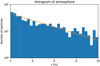 |
Fig. 7 Histogram of the atmosphere above the particle bed populated by about 500 particles. The orange line is a fit with an exponential function, p (z) ~ exp (–z/h), where the scale height h is about 3 m. |
Overview of the performed simulations and their results with regard to the extend of moat and wind tail.
Formation of moat and wind tail
In our simulations we were able to reproduce the formation of moats and wind tails for a wide range of model parameters as summarized in Table 1. The shapes and dimensions of these features, however, depend on the shape of the obstacle and the properties of the particles, which will be discussed in more detail below.
In front of the obstacle, we observe the formation of a moat. As viewed from above, the moat’s shape follows the contour of the obstacle, and its width (in x-direction) is typically larger than its depth, both being on the order of 0.1 m. Behind the boulder, we observe the formation of a wind tail-shaped elevation. The highest point of this elevation is located directly adjacent to the boulder and decreases with distance from it. The wind tail can reach a height that is nearly identical to the height of the obstacle. Additionally, we sometimes also observe a smaller deposition in front of the boulder.
For our reference case with the parameter set given in Sect. 3.2, the evolution of the surface is shown in Fig. 8 after removal of particles from the granular atmosphere, that is when their velocities exceed a certain threshold (0.01ms−1). Surface profiles along the x- (Fig. 8, middle panel) and y-axis (bottom left panel) have been obtained from superimposing the granular surface with a grid and providing a statistically robust measure to determine the surface level at the grid’s sampling points: We divided the surface into overlapping quadratic patches at intervals of 0.2 m in x- and y-direction with sizes of 0.4 m × 0.4 m. For each patch, we removed free particles not in direct contact with those lying underneath, and defined the surface level as the scaled 0.98-quantile  with α = 0.98 and Qα the α-quantile) of the z-coordinates of the remaining particles. This procedure assumes a nearly constant particle number density with z in the particle bed and was found to provide a similar surface level as one would obtain by visually estimating this elevation from cuts of 3D representations of the particle bed (Fig. 8, top panel). To obtain the time evolution of the surface, we performed this analysis for several stages after starting the introduction of the particle wind. Here, the (unscaled) time coordinate was converted into an integrated areal dust flux density F (mass per square meter) describing the total dust mass per square meter that has been inserted into the simulation domain. Neglecting the comparatively few particles in the atmosphere, this corresponds to the spatially averaged mass per square meter deposited on the surface up to that point in time. For each of the considered stages, we determined the minimum elevation of all profiles in front of the obstacle and the maximum elevation behind the obstacle and subtracted a reference surface level (determined as the scaled 0.98-quantile of the outer part of the simulation domain that is less affected by the obstacle) to obtain the relative height of the wind tail and the relative depth of the moat (bottom right panel). We note that in the simulations there is also a small increase (by about 20%) in the bulk density of the upper surface layer (few particle radii) after the introduction of the particle wind, which results from a compaction of the near-surface material by the impacting particles and the resulting perturbation waves. This effect is most likely enhanced in the simulation due to the large size of our particles.
The wind tail is formed by the indirect flux of ejected particles moving surface material into the shielded region behind the boulder rather than due to the erosion of the surrounding area. This is illustrated in Fig. 8, middle panel, where it can be seen that the surface level behind the boulder continually rises everywhere with time. The smaller deposition in front of the boulder possibly results from slow ejected particles getting stopped at and falling down from the boulder’s front face or particles getting “trapped” in the edge when impacting close to the foot of the boulder.
Minimum flux for moat formation
Wind tail and moat develop quickly directly after the onset of the particle wind, and both reach about 50% of their maximum height or depth with respect to the corresponding reference surface level after the insertion of a total of about 50 kg m−2 of dust. From there onward, their growth continues up to an inserted total dust mass of about 250 kg m−2. At this point the top of the wind tail has almost reached the upper edge of the boulder, and further growth of the wind tail is prevented by the ongoing rise of the reference surface level. Across all simulations, the lower limit to the integrated areal dust flux density required for the formation of a moat is on the order of 10 kg m−2.
Assuming morphologic changes of dust beds on the cometary surface typically to occur within the order of days to months, an inserted dust mass of 250 kg m−2 translates to a real world flux density on the order of 10−6–10−5 kgm−2 s−1. For a typical wind speed on the order of 0.1–1 ms−1, the density of the wind near the surface of the nucleus can be estimated to be on the order of 10−6–10−4 kg m−3. Comparing this to the particle insertion flux density of  used in our simulations, the calculations have therefore been accelerated by a factor of 10–100 with respect to the real world elapsed time, which has proven to be necessary to perform the simulations within reasonable CPU time.
The total amount of fall back material onto the comet surface for the two years duration of the Rosetta mission has been estimated to range between 1.9–4.5 × 10¹⁰ kg (Pätzold et al. 2019). With a comet surface area of 46.9 km2 (Jorda et al. 2016) this results in a global average of 6.4–15.2 × 10⁻⁶kgm−2 s−1 comparable to the flux density estimated from our simulation.
In the following, we report and discuss the influence of various model parameters on the formation of aeolian-like features including the shape of the obstacle and the mechanical and physical properties of our particles. Figures 9 and 10 show the simulation outcome after the insertion of a particle wind with an integrated flux density of 100 and 250kgm−2, respectively. During that time the number of particles in the simulation domain has increased from initially 140000 to about 190000 and 260 000, raising the equilibrium surface level from z = 0 to about 0.2 m and 0.5 m, respectively. The top left panel shows our reference case, the other panels show cases where one of the model parameters has been changed with respect to the reference case. Each of these simulations was carried out using parallel processing on a modern Intel Broadwell-type Xeon workstation taking 5000–10000 CPU-core hours of processing time per case.
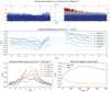 |
Fig. 8 Surface profiles of the reference case (Figs. 9a and 10a). Top panel: cut along the x-axis at y = −0.6 m (because of the asymmetry from rotating the cubic obstacle) of a 3D representation of the particle bed after the insertion of F = 250 kg m−2 of dust. Middle panel: evolution of the surface profile along the x-axis at y = −0.6 m for the reference case and up to a total inserted areal dust mass density of F = 500 kg m−2. The dashed lines are the reference surface levels determined from the less affected outer part of the simulation domain. The obstacle is in the center of the profiles (missing data). Bottom left panel: surface profiles of the wind tail along the y-axis at various distances from the boulder for the case F = 250 kg m−2. Bottom right panel: time evolution of the relative (i.e., with the reference level at this time step subtracted) height of the wind tail (blue solid line) and of the relative depth of the moat (orange solid line). Compare middle and bottom left panels to Fig. 5. |
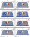 |
Fig. 9 Simulated moats and wind tails around a boulder on the surface of comet 67P, for various sets of model parameters. Each panel shows the situation after the insertion of a particle wind with an integrated areal flux density of 100kgm−2. (a) Reference case: rotated cuboid boulder, particles with radii R = 3 … 6 cm, Young’s modulus Y = 105 Pa, restitution coefficient er = 0.2, triplet of friction coefficients μ/μr/ηr of 1.0/1.0/1.0, cohesive energy density ω = 0.028 J m−2, insertion speed of particle wind iins = 0.5 ms−1. (b–h) Cases, where one of the model parameters (given in the label of the subfigure) has been changed with respect to the reference case. Graphical representation as in Fig. 6. Orange arrows indicate additional local depressions in the low friction case. |
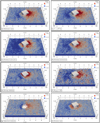 |
Fig. 10 Same as Fig. 9, but after the insertion of a particle wind with an integrated areal flux density of 250 kg m−2. |
Young’s modulus
An increase of Young’s modulus by one order of magnitude with respect to our reference case (Y = 105 Pa) leads to an overall very similar morphology of the moat and the wind tail (Figs. 9b and 10b), with the largest difference being a wider and slightly deeper moat. This shows that although we can only assume our fluffy aggregates to likely have a relatively low Young’s modulus and do not know the exact value of this parameter, our choice has only a limited impact on our results.
Friction
The effect of particle friction was investigated using three test cases with distinct levels of friction: the reference case with medium friction (triplet of friction coefficients – sliding friction μ/rolling friction μr/viscous damping ηr – of 1.0/1.0/1.0, Figs. 9a and 10a), one case with lower (coefficients 0.1/0.1/0.1, Figs. 9c and 10c) and another one with higher friction (coefficients 2.0/2.0/2.0, Figs. 9d and 10d), respectively. The reference case shows a clearly defined, relatively narrow (in x-direction) moat and a large wind tail.
For low friction, the moat is deeper and wider, and it does not have a clearly defined outer edge. The surface is more irregular than in the other cases and there are additional local depressions besides the moat. In total, a noticeably larger amount of surface material has been mobilized, which is due to the low-friction particles being easier to mobilize and harder to stop as they dissipate less kinetic energy when in contact with other grains. For high friction, the moat has a similar depth but larger width compared to the reference case.
In both the low- and high-friction case, the wind tail is somewhat smaller than in the reference case, because low-friction particles are also harder to demobilize and typically form lower wider piles of material and possibly because high-friction particles carry away other particles from the pile. The mobilization of a larger amount of surface material in the low- and high-friction cases is also reflected in the density of the atmosphere, which is about 2–3 times more densely populated compared to the reference case. In this way, the reference case constitutes or is close to a local extremum, leading to the highest wind tails and least dense atmospheres.
Cohesion
In general, stronger cohesion more likely keeps surface particles from being ejected by impinging particles. For a quantitative analysis of the effect of cohesion, we consider the tensile strength of the bulk material, which depends on the particle sizes and configuration as well as the cohesive energy density ω, see discussion in Kappel et al. (2020). Assemblies of larger spherical particles are less stable, because the tensile strength of the material scales inversely with particle size (∝R−1). The number of contacts between two particle layers scales with R−2, while in the DMT model the cohesive force of a single contact scales with R. This means that increasing the cohesive energy density ω or decreasing the particle size R by one order of magnitude increases the tensile strength of the bulk material by a factor of ten.
The tensile strength of the bulk material can also be estimated by a numerical tensile strength test (Kappel et al. 2020). For the reference particle sizes used in our simulations (radii of 3–6 cm) and the reference surface energy density of ω = 0.028 J m−2, the tensile strength is on the order of 0.1 Pa. An increase of the tensile strength by one order of magnitude (Figs. 9e and 10e), that is by decreasing the particle size by a factor of ten and applying coarse-graining by the same factor, significantly reduced the extend of the moat and the wind tail. In comparison to the tensile strength required for the stability of overhanging cliffs on 67P on the order of 1–10Pa (Attree et al. 2018; Groussin et al. 2015), the tensile strength of our material is roughly one order of magnitude smaller, which is plausible considering our material consists of air fall particles, while cliffs are composed of more consolidated material.
Wind particle size
Keeping the particle sizes in the initial particle bed unchanged, the surface erosion increases with increasing incoming particle sizes. When the impinging particles are significantly larger than the particles in the bed, small craterlike features or distinct streaks can be formed in addition to the general erosion, and the surface can become uneven (Figs. 9f and 10f). On the other hand, incoming particles significantly smaller than particles in the bed will cause no erosion at all, because they are not able to eject any surface particles and are just scattered by the surface or even caught by it, depending on cohesion and friction. After settling they raise the average surface level.
67P surface observations of a moat in front of an obstacle and a wind tail behind it in the absence of craters or an uneven morphology indicate that the sizes of the incoming particles are in the same order as those of the surface particles. This suggests that the particles in the bed may originate from the same incoming particle stream in the first place. A change in the sizes of the incoming particles could be related to a change in the emission mode or place.
Shape of obstacle
From the slope and extent of the wind tail-like feature one can purely geometrically infer the local inclination of the incoming particle stream assuming the stream direction and wind tail slope are the same (as has been done in the Mottola et al. 2015 model). The length of the wind tail allows an estimate of the inclination by simple triangulation when knowing the height of the obstacle with respect to the local reference level. However, the slope is also sensitive to interparticle forces like cohesion and rolling friction, as it is related to the (static) angle-of-repose of the material.
While a wind tail was visible in all our simulations, the existence of a moat depends on the shape of the obstacle. An obstacle with the shape of a half-sphere (like a dome) distributes the incoming particles into many directions, which makes it more difficult for a moat to be formed (Figs. 9g and 10g). To a lesser extent the same applies to an upright cylinder. Choosing a cube with one side (called the “front face”) facing the incoming particle stream, the particles impinging on this face are simply reflected into the particle bed and not laterally distributed. This additional erosion in front of the boulder can lead to a more effective moat formation. Also, when the cube is rotated around its vertical axis, moats can be formed not (only) in front of the boulder but also along the boulder walls. Therefore we suggest that aeolian-like features also represent form and orientation of the front face of the obstacle.
Velocity of incoming particle stream
If the incoming particles have just 20% of the orbital velocity (0.1 m s−1), the surface erosion is minimal and the particles are rather just deposited near their first point of contact with the surface. At the front face of the obstacle they are reflected leading to additional deposition in front of the obstacle. Furthermore, they cannot reach the region behind it, leading to less deposition there. Consequently, an inverted moat-wind tail morphology can develop, with the moat behind the obstacle and the wind tail-like feature in front. However, the depositional feature is broader than the obstacle in contrast to the not-inverted case. The observed features on the 67P surface indicate the not-inverted case to be the usual one on the nucleus, corroborating the argument about the orbital velocity of the incoming particle stream.
Changing the individual insertion velocities by small random terms (direction and velocity) does not change our results. A change of inclination of the particle stream causes the wind tail to adapt to the according geometry.
Erosion case
In the simulation cases discussed so far, the steady insertion of particles led to a slowly but continually rising reference surface, which would eventually completely bury the boulder and obliterate the surface features associated with it. We recall that this is not an unphysical but an actually observed effect that results from the transfer of material from one side of the nucleus to another, here modeled by the particle wind and the assumption that our simulation domain is part of an infinitely extended plane composed of many such domains modeled by the use of periodic boundary conditions. The “opposite” case is the assumption that our simulation domain is in some way, for example, by long distances, being on a plateau, or shielded by cliffs, isolated from a larger particle bed. We performed such a simulation and modeled the absence of the ejecta flux from neighboring cells by keeping the periodic geometry but removing all ejecta whose ejection range exceeded half the basic simulation dimension in x- or y-direction. This way we still avoid the strong boundary effects in absence of periodic boundary conditions and are able to simulate a net erosion of the particle bed, a situation that has been actually observed on the nucleus surface (Hu et al. 2017).
In the erosion case (Figs. 9h and 10h), the perpetual removal of far-reaching ejecta leads to a very slowly decreasing reference surface level, which would eventually excavate the initially buried base of the boulder. Despite the different evolution of the surface level, it is still possible to form a moat. The wind tail, however, is less developed, and its formation process is different from that of the deposition case. In the erosion case, the wind tail mostly results from the erosion of the area not shielded by the boulder as the indirect flux of slow ejecta is smaller. The extent of the wind tail is noticeably smaller (about half in every dimension) and, in particular, it is lower than the deposition in front of the obstacle, creating the impression of an inverted moat-wind tail morphology. The timescale for the formation of the wind tail is about the same in the erosion case (Fig. 11), but this depends on the ejecta speed distribution, which determines the fraction of particles launched beyond the domain boundaries that are lost. As a result, the observed extended wind tails on the 67P surface are less compatible with the erosion case and indicate the depositional case to be the usual one on the nucleus.
5 Conclusions and outlook
In this work, we have applied the DEM to perform numerical simulations of dynamical surface processes on comet 67P in order to investigate local transport processes and mechanical properties of the surface material. We modeled air fall particles as polydisperse spheres consisting of a mixture of dust and water ice and took into account the ambient surface acceleration, the Hertz contact model, translational and rolling friction, and cohesion. To enable the modeling of large scenarios with realistically small constituent particles, we employed the coarse-graining technique. Recently, we applied the DEM method to investigate morphologies of boulders and cliffs on 67P (Kappel et al. 2020). Now we applied our model to study the formation of moat- and wind tail-like features around exposed boulders in a particle bed as observed for instance by Mottola et al. (2015).
With our DEM model, we constructed a rectangular cometary particle bed with a boulder in its center and an oblique particle wind coming from above the obstacle. We investigated two limiting cases – a deposition case, where we assumed that our simulation domain is part of an infinitely extended plane composed of many such domains and modeled the indirect flux from the neighboring domain using periodic boundary conditions; and an erosion case, where we instead assumed that our simulation domain constitutes a somewhat isolated part on the nucleus and removed all ejecta whose ejection range exceeded half the basic horizontal domain dimensions. The differences to the simpler cell-based model of Mottola et al. (2015), which only considers erosion, are the re-distribution of mobilized surface particles and physical or geometric effects like friction, cohesion, rotation, compression waves, and porosity.
In the deposition case, where no particles are lost, it can been seen that, despite a slowly but continually rising surface level, the formation of the wind tail occurs entirely due to the indirect flux of ejected particles moving surface material into the region behind the boulder shielded from the particle stream rather than due to the erosion of the surrounding area suggested by Mottola et al. (2015). Here, the moat and wind tail reached their maximum depth or height after being exposed to an integrated areal dust flux density of about 250 kg m−2. Based on the timescale of morphological changes on the surface of comet 67P inferred from Rosetta images, the density of the wind near the surface was estimated to be on the order of 10−6−10−4 kgm−3.
In the erosion case, we also observed the formation of a wind tail and a moat. However, the process generating the wind tail is different: it mostly forms as a result of shielding of the preexisting particle bed from the particle stream as the flux of ejecta accumulating in the region behind the boulder is smaller. The moat develops as a result of increased erosion as observed in the deposition case. This scenario is comparable to the model by Mottola et al. (2015).
In our simulations, we were able to reproduce the formation of a moat and wind tail for a wide range of model parameters. However, a clearly defined, relatively narrow moat and an extended wind tail as typically observed on 67P was obtained only for a medium level of particle friction in the depositional case. Both lower and higher friction levels resulted in moats with less defined edges. The erosional case led to much smaller wind tails creating the impression of an inverted moat-wind tail morphology that is less compatible with observations. Reasonable changes to Young’s modulus within the range of 105 Pa to 106 Pa impacted the morphology of the moat or the wind tail only to a small degree. However, the extend of the moat and the wind tail was significantly reduced when the tensile strength of the material, given by the material’s constituent sizes, internal structures and/or cohesive energy density, was increased from 0.1 Pa to 1 Pa. A cube was the most effective shape for the formation of a moat, while obstacles with rounder shapes, a cylinder and, in particular, a half-sphere (like a dome), distributed the incoming particles into many directions, which made it more difficult for a moat to form. Therefore, for future analyses of the particle stream and bed conditions based on wind tail and moat morphology, we suggest, in cases where discernible from the imaging data, to also include form and orientation of the front face of the obstacle, in addition to obstacle height and moat and wind tail geometry. Particles responsible for the formation of these features likely originate from distant locations on the nucleus as impactors significantly slower than the orbital velocity failed to reproduce the observed morphologies.
Our simulations have shown that morphologic investigations of wind tails and moats can be used to constrain physical parameters of cometary material and air fall processes. This method can be adapted to future morphologic investigations of features on comets as well as in the laboratory and is the base for more advanced simulations.
As the next step (Kappel et al. 2018b,a), we plan to study further surface processes on comet 67P, for instance the formation of fracture polygons (possibly induced by thermal stress) that have been observed in many places where consolidated material is exposed on the nucleus surface (Auger et al. 2018). We also intend to include Monte-Carlo-based modeling of sublimation and recondensation of volatiles and Knudsen gas flow through the surface layer, which will provide us with a tool to investigate more complex scenarios such as triggers and early phases of cometary outbursts as well as other volatile-related processes, on comet 67P and other small Solar System bodies.
 |
Fig. 11 Surface profiles of the erosion case (Figs. 9h and 10h). Representation as in Fig. 8, but up to a total inserted areal dust mass density of F = 1000 kg m−2. |
Acknowledgements
We very much thank Laurent Jorda for providing the DTM of the Agilkia landing site. This work is part of the research project “The Physics of Volatile-Related Morphologies on Asteroids and Comets”. M.S., D.K., and K.O. would like to gratefully acknowledge the financial support and endorsement from the DLR Management Board Young Research Group Leader Program and the Executive Board Member for Space Research and Technology.
References
- Ai, J., Chen, J.-F., Rotter, J. M., & Ooi, J. Y. 2011, Powder Technol., 206, 269 [CrossRef] [Google Scholar]
- Attree, N., Groussin, O., Jorda, L., et al. 2018, A&A, 611, A33 [NASA ADS] [CrossRef] [EDP Sciences] [Google Scholar]
- Auger, A.-T., Groussin, O., Jorda, L., et al. 2018, Icarus, 301, 173 [Google Scholar]
- Biele, J., Ulamec, S., Maibaum, M., et al. 2015, Science, 349, aaa9816 [Google Scholar]
- Bierwisch, C., Kraft, T., Riedel, H., & Moseler, M. 2009, J. Mech. Phys. Solids, 57, 10 [NASA ADS] [CrossRef] [Google Scholar]
- Brilliantov, N. V., Spahn, F., Hertzsch, J.-M., & Pöschel, T. 1996, Phys. Rev. E, 53, 5382 [NASA ADS] [CrossRef] [Google Scholar]
- Davidsson, B. J. R., Birch, S., Blake, G. A., et al. 2020, Icarus, 354, 114004 [Google Scholar]
- El-Maarry, M. R., Groussin, O., Keller, H. U., et al. 2019, Space Sci. Rev., 215, 36 [Google Scholar]
- El-Maarry, M. R., Thomas, N., Giacomini, L., et al. 2015, A&A, 583, A26 [NASA ADS] [CrossRef] [EDP Sciences] [Google Scholar]
- El-Maarry, M. R., Groussin, O., Thomas, N., et al. 2017, Science, 355, 1392 [Google Scholar]
- Golombek, M. P., Crumpler, L. S., Grant, J. A., et al. 2006, J. Geophys. Res. Planets, 111, E02S07 [Google Scholar]
- Greeley, R., Kraft, M., Sullivan, R., et al. 1999, J. Geophys. Res., 104, 8573 [NASA ADS] [CrossRef] [Google Scholar]
- Greeley, R., Bridges, N. T., Kuzmin, R. O., & Laity, J. E. 2002, J. Geophys. Res. Planets, 107, 5005 [NASA ADS] [CrossRef] [Google Scholar]
- Groussin, O., Jorda, L., Auger, A. T., et al. 2015, A&A, 583, A32 [NASA ADS] [CrossRef] [EDP Sciences] [Google Scholar]
- Heim, L.-O., Blum, J., Preuss, M., & Butt, H.-J. 1999, Phys. Rev. Lett., 83, 3328 [NASA ADS] [CrossRef] [Google Scholar]
- Hertz, H. 1882, J. reine angewandte Mathematik, 92, 156 [CrossRef] [Google Scholar]
- Horányi, M., Szalay, J. R., Kempf, S., et al. 2015, Nature, 522, 324 [CrossRef] [Google Scholar]
- Hu, X., Shi, X., Sierks, H., et al. 2017, A&A, 604, A114 [NASA ADS] [CrossRef] [EDP Sciences] [Google Scholar]
- Jorda, L., Gaskell, R., Capanna, C., et al. 2016, Icarus, 277, 257 [Google Scholar]
- Kappel, D., Otto, K., Oklay, N., et al. 2018a, Eur. Planet. Sci. Cong., 12, EPSC2018 [Google Scholar]
- Kappel, D., Otto, K., Oklay-Vincent, N., et al. 2018b, in Lunar and Planetary Inst. Technical Report, 49, Lunar and Planetary Science Conference, 2696 [Google Scholar]
- Kappel, D., Sachse, M., Haack, D., & Otto, K. 2020, A&A, 641, A19 [NASA ADS] [CrossRef] [EDP Sciences] [Google Scholar]
- Keller, H. U., Barbieri, C., Lamy, P., et al. 2007, Space Sci. Rev., 128, 433 [Google Scholar]
- Keller, H. U., Mottola, S., Hviid, S. F., et al. 2017, MNRAS, 469, S357 [Google Scholar]
- Kloss, C., Goniva, C., Hager, A., Amberger, S., & Pirker, S. 2012, Prog. Comput. Fluid Dyn., 12, 140 [CrossRef] [Google Scholar]
- Kramer, T., & Noack, M. 2015, ApJ, 813, L33 [Google Scholar]
- Krivov, A. V., Sremčević, M., Spahn, F., Dikarev, V. V., & Kholshevnikov, K. V. 2003, Planet. Space Sci., 51, 251 [NASA ADS] [CrossRef] [Google Scholar]
- Krüger, H., Krivov, A. V., Hamilton, D. P., & Grün, E. 1999, Nature, 399, 558 [CrossRef] [Google Scholar]
- Krüger, H., Krivov, A. V., Sremčević, M., & Grün, E. 2003, Icarus, 164, 170 [CrossRef] [Google Scholar]
- Lai, I.-L., Ip, W.-H., Su, C.-C., et al. 2016, MNRAS, 462, S533 [NASA ADS] [CrossRef] [Google Scholar]
- Mannel, T., Bentley, M. S., Boakes, P. D., et al. 2019, A&A, 630, A26 [NASA ADS] [CrossRef] [EDP Sciences] [Google Scholar]
- Mottola, S., Arnold, G., Grothues, H.-G., et al. 2007, Space Sci. Rev., 128, 241 [NASA ADS] [CrossRef] [Google Scholar]
- Mottola, S., Arnold, G., Grothues, H. G., et al. 2015, Science, 349, 2.232 [NASA ADS] [CrossRef] [Google Scholar]
- Muller, V., Derjaguin, B., & Toporov, Y. 1983, Colloids Surf., 7, 251 [CrossRef] [Google Scholar]
- Otto, K. A., Tirsch, D., Mottola, S., et al. 2017, in Asteroids, Comets, Meteors (UK: Wayland) [Google Scholar]
- Pätzold, M., Andert, T., Hahn, M., et al. 2016, Nature, 530, 63 [CrossRef] [Google Scholar]
- Pätzold, M., Andert, T.P., Hahn, M., et al. 2019, MNRAS, 483, 2337 [CrossRef] [Google Scholar]
- Potyondy, D., & Cundall, P. 2004, Int. J. Rock Mech. Mining Sci., 41, 1329 [Google Scholar]
- Preusker, F., Scholten, F., Matz, K. D., et al. 2017, A&A, 607, L1 [NASA ADS] [CrossRef] [EDP Sciences] [Google Scholar]
- Sachse, M., Schmidt, J., Kempf, S., & Spahn, F. 2015, J. Geophys. Res. Planets, 120, 1847 [NASA ADS] [CrossRef] [Google Scholar]
- Spohn, T., Knollenberg, J., Ball, A. J., et al. 2015, Science, 349, aab0464 [Google Scholar]
- Sremcevic, M., Krivov, A. V., & Spahn, F. 2003, Planet. Space Sci., 51, 455 [CrossRef] [Google Scholar]
- Thomas, N., Davidsson, B., El-Maarry, M. R., et al. 2015a, A&A, 583, A17 [NASA ADS] [CrossRef] [EDP Sciences] [Google Scholar]
- Thomas, N., Davidsson, B., El-Maarry, M. R., et al. 2015b, Lunar Planet. Sci. Conf., 1712 [Google Scholar]
- Thomas, N., Sierks, H., Barbieri, C., et al. 2015c, Science, 347, aaa0440 [Google Scholar]
- Tirsch, D., Otto, K. A., Mottola, S., et al. 2017a, Eur. Planet. Sci. Cong., 11 [Google Scholar]
- Tirsch, D., Otto, K. A., Mottola, S., et al. 2017b, in 5th International Planetary Dunes Workshop, 1961, 3011 [Google Scholar]
All Tables
Overview of the performed simulations and their results with regard to the extend of moat and wind tail.
All Figures
|
Fig. 1 Mapping of aeolian-like morphologies on OSIRIS image data at the Agilkia touchdown 1 site, as an example for the 362 images analyzed. The orientation of the moats, wind tails, and smooth ridges indicate material transport from the same source direction, i.e., from the lower right to the upper left of this image (OSIRIS image NAC_2014-11-12T15.43.51.584Z; image credit: MPS/UPD/LAM/IAA/SSO/INTA/UPM/DASP/IDA). |
| In the text | |
|
Fig. 2 Wind tails and moats on different planetary bodies. (a) Wind tails associated with vegetation acting as obstacles at Grand Falls Dune Field, Arizona, USA (Photo: D. Tirsch). (b) Boulder “Barnacle Bill” at the Mars Path Finder landing site. This 43-by-22-cm-sized rock is associated with a distinctive moat to its right and a wind tail to its left (subset of MPF image 81008 with parts of the Sojourner rover at the lower right). (c) 5-m-sized boulder at Philae’s first touchdown site “Agilkia” on comet 67P. White dashed lines trace the shape of the moat and the wind tail associated with this boulder (subset of ROLIS image ROL_FS3_141112153316_336_02). (d) Sketch showing the typical shape of a moat and a wind tail associated with an obstacle. Blue arrows indicate the wind direction in panels a, b, and d as well as the transport direction of air fall particles in panel c. |
| In the text | |
|
Fig. 3 Distribution of boulders (red spheres) with wind tails (arrows) on 67P projected onto a digital shape model by Preusker et al. (2017) with 67P’s morphologic regions outlined (El-Maarry et al. 2015). The arrows’ directions represent wind tail orientation including inclination and thus illustrate the presumed directions of the incoming particle streams, and their colors indicate the wind tail lengths. The boulder sizes are matched by the red sphere sizes. Most of these features are found in the Ma’at and Serqet regions, which are located at “the top of the head”, i.e., the northern part of the small lobe (Otto et al. 2017). |
| In the text | |
|
Fig. 4 Scatter plot of boulder height and wind tail length. The orange line is a linear fit with a slope of 0.94. |
| In the text | |
|
Fig. 5 Morphometry of wind tails at the Agilkia landing site. (a and b): perspective views showing the two boulders based on OSIRIS images and DTM data (Jorda et al. 2016). Colors in a encode elevations from – 16 m (blue) to + 15 m (red). Labels in b indicate boulder sizes. The lateral and vertical DTM resolutions are about 35 and 10 cm per pixel, respectively. (c–f): longitudinal and transverse cross sections of the wind tails (and the moat) associated with the two boulders at Agilkia (Tirsch et al. 2017a). The size of the wind tail in profile (ƒ) is at the limit of the DTM resolution which is the reason for the step-like shape of the profile. |
| In the text | |
|
Fig. 6 Construction of an obstacle in the center of a cometary particle bed made up of 140 000 polydisperse spheres consisting of a porous dust-ice mixture with a volume ratio of 2:1, and exposure to a particle wind. Top row: construction of the particle bed. (a) Loose filling of a horizontal layer at the bottom of the simulation domain with non-contacting randomly positioned and sized (chosen from eight discrete sizes) spherical particles. (b) Removal of particles in the center region and insertion of an obstacle built of wall elements. (c) Compaction of the particle layer to the bulk mass density and porosity of comet 67P and removal of particles above the given layer thickness. Bottom row: (d–f) several stages after the introduction of the particle wind. Particles from the granular atmosphere are removed for better representation. The color bar is adapted to the changing overall level of the particle bed. |
| In the text | |
|
Fig. 7 Histogram of the atmosphere above the particle bed populated by about 500 particles. The orange line is a fit with an exponential function, p (z) ~ exp (–z/h), where the scale height h is about 3 m. |
| In the text | |
|
Fig. 8 Surface profiles of the reference case (Figs. 9a and 10a). Top panel: cut along the x-axis at y = −0.6 m (because of the asymmetry from rotating the cubic obstacle) of a 3D representation of the particle bed after the insertion of F = 250 kg m−2 of dust. Middle panel: evolution of the surface profile along the x-axis at y = −0.6 m for the reference case and up to a total inserted areal dust mass density of F = 500 kg m−2. The dashed lines are the reference surface levels determined from the less affected outer part of the simulation domain. The obstacle is in the center of the profiles (missing data). Bottom left panel: surface profiles of the wind tail along the y-axis at various distances from the boulder for the case F = 250 kg m−2. Bottom right panel: time evolution of the relative (i.e., with the reference level at this time step subtracted) height of the wind tail (blue solid line) and of the relative depth of the moat (orange solid line). Compare middle and bottom left panels to Fig. 5. |
| In the text | |
|
Fig. 9 Simulated moats and wind tails around a boulder on the surface of comet 67P, for various sets of model parameters. Each panel shows the situation after the insertion of a particle wind with an integrated areal flux density of 100kgm−2. (a) Reference case: rotated cuboid boulder, particles with radii R = 3 … 6 cm, Young’s modulus Y = 105 Pa, restitution coefficient er = 0.2, triplet of friction coefficients μ/μr/ηr of 1.0/1.0/1.0, cohesive energy density ω = 0.028 J m−2, insertion speed of particle wind iins = 0.5 ms−1. (b–h) Cases, where one of the model parameters (given in the label of the subfigure) has been changed with respect to the reference case. Graphical representation as in Fig. 6. Orange arrows indicate additional local depressions in the low friction case. |
| In the text | |
|
Fig. 10 Same as Fig. 9, but after the insertion of a particle wind with an integrated areal flux density of 250 kg m−2. |
| In the text | |
|
Fig. 11 Surface profiles of the erosion case (Figs. 9h and 10h). Representation as in Fig. 8, but up to a total inserted areal dust mass density of F = 1000 kg m−2. |
| In the text | |
Current usage metrics show cumulative count of Article Views (full-text article views including HTML views, PDF and ePub downloads, according to the available data) and Abstracts Views on Vision4Press platform.
Data correspond to usage on the plateform after 2015. The current usage metrics is available 48-96 hours after online publication and is updated daily on week days.
Initial download of the metrics may take a while.