| Issue |
A&A
Volume 661, May 2022
|
|
|---|---|---|
| Article Number | L5 | |
| Number of page(s) | 5 | |
| Section | Letters to the Editor | |
| DOI | https://doi.org/10.1051/0004-6361/202243691 | |
| Published online | 17 May 2022 | |
Letter to the Editor
Spectral evidence of solar neighborhood analogs in CALIFA galaxies
1
Instituto de Astronomía, Universidad Nacional Autónoma de México, A. P. 70-264, C.P., 04510 Mexico, DF, Mexico
e-mail: This email address is being protected from spambots. You need JavaScript enabled to view it.
2
McDonald Observatory, The University of Texas at Austin, 1 University Station, Austin, TX 78712, USA
Received:
1
April
2022
Accepted:
27
April
2022
Abstract
Aims. We introduce a novel nonparametric method to find solar neighborhood analogs (SNAs) in extragalactic integral field spectroscopic surveys. The main ansatz is that the physical properties of the solar neighborhood (SN) should be encoded in its optical stellar spectrum.
Methods. We assume that our best estimate of such a spectrum is the one extracted from the analysis performed by the Code for Stellar properties Heuristic Assignment (CoSHA) from the MaStar stellar library. It follows that finding SNAs in other galaxies consist in matching, in a χ2 sense, the SN reference spectrum across the optical extent of the observed galaxies. We applied this procedure to a selection of CALIFA galaxies, by requiring a close to face-on projection, relative isolation, and non-active galactic nucleus. We explore how the local and global properties of the SNAs (stellar age, metallicity, dust extinction, mass-to-light ratio, stellar surface mass density, star-formation density, and galactocentric distance) and their corresponding host galaxies (morphological type, total stellar mass, star-formation rate, and effective radius) compared with those of the SN and the Milky Way (MW).
Results. We find that SNAs are located preferentially in S(B)a–S(B)c galaxies, in a ring-like structure, which radii seem to scale with the galaxy size. Despite the known sources of systematics and errors, most properties present a considerable agreement with the literature on the SN. We conclude that the solar neighborhood is relatively common in our sample of SNAs. Our results warrant a systematic exploration of correlations among the physical properties of the SNAs and their host galaxies. We reckon that our method should inform current models of the galactic habitable zone in our MW and other galaxies.
Key words: methods: statistical / solar neighborhood / galaxies: stellar content
© A. Mejía-Narváez et al. 2022
 Open Access article, published by EDP Sciences, under the terms of the Creative Commons Attribution License (https://creativecommons.org/licenses/by/4.0), which permits unrestricted use, distribution, and reproduction in any medium, provided the original work is properly cited.
This article is published in open access under the Subscribe-to-Open model. This email address is being protected from spambots. You need JavaScript enabled to view it. to support open access publication.
1. Introduction
Studies of the solar vicinity, whether this vicinity involves only a few hundred stars around the Sun or the whole Milky Way (MW), have the potential to answer fundamental questions about the formation of our galaxy and its satellites (e.g., Helmi et al. 2018; Ruiz-Lara et al. 2020), the formation of the Sun and its planets (e.g., Raymond et al. 2020), and ultimately the physical conditions needed to sustain life as we know it (e.g., Gonzalez et al. 2001). In an attempt to characterize the most likely zone in our MW with the conditions needed for life to sprout and thrive, Gonzalez et al. (2001) introduced the Galactic habitable zone (GHZ), including a set of values for relevant physical properties that should constrain the habitability of different locations in the MW and in other galaxies. They suggested that the GHZ is a ring-like structure located in the thin disk that extends with time toward the outskirts of the disk.
The GHZ was latter explored by Lineweaver et al. (2004). Based on chemical evolution models, those authors argued that the width of the ring should grow as a function of cosmic time, due to the inside-out evolution of the disk (from 6 to 10 kpc). Similar results were found by Spitoni et al. (2014, 7–9 kpc). By considering the stellar density, Prantzos (2008) found that the most probable GHZ is in the inner disk (∼3 kpc), which was later confirmed by Gowanlock et al. (2011). In the cosmological context, the GHZ has also been characterized through simulations, with predictions that our Sun is not in the most probable GHZ, but instead being either in the lower limit of the galactocentric distance distribution (e.g., Vukotić et al. 2016) or in the upper limit (e.g., Forgan et al. 2017) and, more interestingly, not in the most likely host galaxy type (e.g., Zackrisson et al. 2016; Gobat & Hong 2016). Such theoretical results thus far lack solid observational support.
The physical properties of the MW and the solar neighborhood (SN) have been widely studied in different surveys, such as SEGUE (Yanny et al. 2009), APOGEE (Holtzman et al. 2015), GALAH (De Silva et al. 2015), and Gaia (Gaia Collaboration 2018a). As a matter of fact, we have drawn a clear picture of our MW (see Bland-Hawthorn & Gerhard 2016, for a review; BH16 hereafter) and the SN (e.g., Buder et al. 2019); this is knowledge that has been fed to simulations to reproduce observations with success (e.g., Prantzos et al. 2018). At global (i.e., the typical scale of a galaxy) and extragalactic scales, we have sampled hundreds of MW analogs in large surveys (e.g., Fraser-McKelvie et al. 2019; Boardman et al. 2020), leading to the conclusion that the MW is common among its analogs, but relatively rare among a complete sample of galaxies of the local Universe. At local scales (i.e., kiloparsec scales and below), however, we have yet to make progress in finding SN analogs (SNAs) in extragalactic surveys.
In this Letter, we seek to bridge the gap between simulations of the evolution of the SN and the whole MW, and current observations of its physical properties. Therefore, we used a nonparametric method to find SNAs in other galaxies that have been observed using integral field units (IFUs). The main premise of our endeavor is that the physics of our SN is encoded in its integrated optical spectrum. Since we know for a fact that in our SN life exists, it follows that the physical conditions defining our portion of the GHZ should also be encoded in such a spectrum. In particular, we study how similar are the SNAs properties, as found in other galaxies, to our own SN, how typical or atypical these regions are and the type of galaxies – morphologically speaking – where SNAs are more likely to be found. Moreover we characterize the galactocentric distance distribution of the SNAs and seek to determine if it scales with the host galaxy size. A natural follow-up is to know if the Sun is in an expected location or if it is an outlier in this distribution. This Letter is organized as follows: in Sect. 2 we describe the samples and analysis methods; in Sect. 3 we present our main findings; and finally we discuss and conclude in Sect. 4.
2. Data and analysis
2.1. MaStar as a spectroscopic sample of solar neighborhood stars
MaStar (Yan et al. 2019) is a stellar library for the MaNGA survey (Bundy et al. 2015; Drory et al. 2015). Mejía-Narváez et al. (2021, hereafter MN21) labeled ∼22 k unique stars in this library using CoSHA, a heuristic machine learning approach. One by-product of the analysis in MN21 that is relevant to the present Letter is the partial volume correction implemented using the color-magnitude diagram (CMD) sampled by Gaia DR2 (Gaia Collaboration 2018a). The Gaia survey has been implemented in the recent past to analyze the solar neighborhood properties (e.g., Ding et al. 2019; Sollima 2019; Gontcharov & Mosenkov 2021; Alzate et al. 2021); therefore, it is a good survey to draw a photometric sample (e.g., Evans et al. 2018) of the solar surroundings. Knowing this, MN21 calculated a partial volume correction using the following relation:
 (1)
(1)
where CMDMaStar and CMDGaia represent the PDF distribution of stars in the extinction corrected CMD sampled by MaStar and Gaia (Gaia Collaboration 2018b), respectively (e.g., Wall & Jenkins 2003; Rodríguez-Puebla et al. 2017; Sánchez et al. 2019). The “partial” character of this volume correction comes from the fact that Gaia is not a complete sample of the stars in the solar neighborhood. However it is, to the best of our knowledge, the most complete sample to date. The fact that the volume-corrected distributions of MaStar chemical abundances ([Fe/H] and [α/Fe]) resemble those from independent studies in the SN (cf. Fig. 9 in MN21) is encouraging. Hence, we can assert that the weighted averaged MaStar spectrum with weights Vcor is, by design, our best estimate for the solar neighborhood optical spectrum. In the following, we allude to this spectrum,  , as our spectroscopic reference of the solar neighborhood or simply the SN spectrum.
2.2. A solar neighborhood definition
The solar neighborhood is usually defined as the volume enclosed within a set radius around the Sun. There is no consensus, however, on the value of such radius and the literature on MW studies spans ranges from a few tens of parsecs to 1 kpc, depending on the specific subject of research (e.g., Vergely et al. 1998; Aniyan et al. 2016). Here, we define the radial scale of the solar neighborhood a posteriori as the standard deviation of the volume corrected distance distribution of stars in the MaStar sample: rSN = 1.24 kpc. This definition is consistent with the upper limit quoted above. It is also consistent with the typical physical resolution in the CALIFA sample at the average redshift ∼0.8 kpc (FWHM = 0.3–1.8 kpc), which is indeed a convenient coincidence for the current study (although it does not impose a strong limitation). We note that this definition is purely observational and that we may have a contribution from halo stars. However, as we see below, any potential bias due to this selection should be accounted for by the projection effects of CALIFA galaxies.
2.3. A golden sample from CALIFA
CALIFA (Sánchez et al. 2012) is an integral field spectroscopic (IFS) survey of ∼1000 galaxies in the nearby universe z ∼ 0.015, which is complete to M⋆ ∼ 1011.4 M⊙ and spanning all morphological types (Walcher et al. 2014; Galbany et al. 2018). We note that CALIFA is the only IFS survey that covers up to 2.5 reff, that is to say most of the optical extension of galaxies is within the field of view (FoV) of the instrument, which is a relevant trait in our study (cf. Table 1 in Sánchez 2020). The physical properties of these galaxies have been estimated and summarized using the Pipe3D pipeline (Sánchez et al. 2016a,b), whose data products have been extensively used in numerous publications (e.g., López-Cobá et al. 2020; Mejía-Narváez et al. 2020; Valerdi et al. 2021; Barrera-Ballesteros et al. 2021; Espinosa-Ponce et al. 2022). We focus our attention on galaxies that are not highly inclined in order to locate SNAs across their optical extent. In particular, we have three requirements for a galaxy to belong to our golden sample: (i) the inclination angle is ≤60 deg, also avoiding known issues (e.g., Ibarra-Medel et al. 2019); (ii) we have a reliable morphological classification; (iii) the galaxy has no evidence of nearby companions, ongoing collisions, or post-merger signatures1; and (iv) the galaxy must not host an active galactic nucleus according to Lacerda et al. (2020). After applying these constraints, our initial sample was reduced to 330 galaxies, (approximately a third) of the original CALIFA sample. This golden selection poses the possibility of finding SNAs in galaxies that hold no a priori resemblance with the MW.
2.4. Finding solar neighborhood analogs
We looked for the SNA across the optical extent of CALIFA galaxies by exploring the spatial distribution of the χ2, in which the observed spectra in each spaxel was compared with our reference spectrum for the SN in the MW (Sect. 2.2). For this purpose, the SN reference spectrum was convolved with a Gaussian function and dust attenuated using the Cardelli et al. (1989) model, following the procedures in pyFIT3D (Lacerda et al. 2022, Eq. (1)). Hence, we accounted for (1) the redshift and velocity rotation of the galaxy; (2) line-of-sight velocity dispersion; and (3) differential extinction due to projection and line-of-sight effects. To further account for the differential physical spatial resolution of each spaxel (∼1″) at the observed galaxy redshift, the CALIFA cubes were convolved with a Gaussian kernel to match the resolution of our SN region (∼1 kpc, Sect. 2.2).
Based on the χ2-matching we performed for each spaxel, we label as SNA those regions in which the  is within the range 0.7–1.3, simultaneously avoiding the spaxels that mismatch our reference spectrum (> 1.3) and those with overestimated uncertainties (< 0.7).
3. Results
Figure 1 summarizes our main results for the following three galaxies hosting SNA regions, as an illustrative example: NGC 5947, NGC 5000, and NGC 309. For each galaxy we show the contour of the likelihood map (![Mathematical equation: $ \mathcal{L}_{ij}\propto\exp{\left[-{\chi_{ij}^2}/2\right]} $](/articles/aa/full_html/2022/05/aa43691-22/aa43691-22-eq4.gif) ) on top of the RGB composite image, highlighting the location of the most likely SNA. In addition we show the corresponding spectra of those regions together with the reference SNA spectrum. We observe that the SNA spectrum of the three example galaxies is well within the uncertainty band, σλ (shaded region), for most of the wavelength range. A higher ℒSNA indicates that the likelihood of finding a SNA within the target galaxy is more concentrated around a specific region. In the top panels of Fig. 1, NGC 5000 shows the most concentrated likelihood of hosting SNA spaxels, with an apparent azimuthal symmetry. At first sight, this pattern is also followed by NGC 5947 and NGC 309, whereby likely SNA spaxels are grouped in a ring-like structure. Interestingly, the radius of such a structure seems to depend on the galaxy’s apparent size. We explore this below.
) on top of the RGB composite image, highlighting the location of the most likely SNA. In addition we show the corresponding spectra of those regions together with the reference SNA spectrum. We observe that the SNA spectrum of the three example galaxies is well within the uncertainty band, σλ (shaded region), for most of the wavelength range. A higher ℒSNA indicates that the likelihood of finding a SNA within the target galaxy is more concentrated around a specific region. In the top panels of Fig. 1, NGC 5000 shows the most concentrated likelihood of hosting SNA spaxels, with an apparent azimuthal symmetry. At first sight, this pattern is also followed by NGC 5947 and NGC 309, whereby likely SNA spaxels are grouped in a ring-like structure. Interestingly, the radius of such a structure seems to depend on the galaxy’s apparent size. We explore this below.
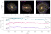 |
Fig. 1. Demonstration of our method for finding SNAs with three sample galaxies in our golden sample. Top panels: RGB (R: 6450 Å, G: 5375 Å, and B: 3835 Å) composite images of galaxies NGC 5947, NGC 5000, and NGC 309 in our golden sample described in Sect. 2.3 which likely hosts SNA regions. The likelihood map is overlaid in each case with contours enclosing the 1σ (solid), 2σ (dashed), and 3σ (dotted), respectively. The location of the maximum likelihood in each case (colored circle) and its galactocentric distance (dashed colored line) are shown. Bottom panel: spectrum corresponding to the maximum likelihood spaxel (solid line in color) along with the propagated (1σ) error spectrum (shaded region). We highlight the regions where the error spectrum was masked out (dotted). The SNA spectrum (gray) calculated as described in Sect. 2.4 is also shown. The resulting χ2 and the likelihood integrated within a circular aperture matching the SN physical scale around the maximum are also shown. |
Repeating the above analysis for each galaxy, we find SNAs in only 61 out of 330 galaxies (∼20%). Table 1 shows the physical properties of the MW and in our solar vicinity (Col. 2) together with those of the host galaxies and the corresponding most likely SNA regions (Col. 3). A detailed exploration of these properties will be presented in a forthcoming study. Here, we present a brief summary of this type of exploration.
Median global and local properties for the MW and the SN, respectively, compared to the SNA hosts’ and regions’ values retrieved in this Letter.
Despite remaining indifferent about the global and local physical properties of potential host galaxies, we find that most likely SNA regions (within 1σ) are more frequent in spiral galaxies ranging Sa–Sc and that these regions seem to lie preferentially in between arms. As a matter of fact, this is the expectation in the MW (Sb–Sbc), where the Sun is known to be located between Perseus and Carina-Sagittarius arms (e.g., BH16). The median global stellar mass (Fig. 2a), log M⋆/M⊙ ∼ 10.91 ± 0.26, and star-formation rate (SFR; Fig. 2b), log ψ⋆ ∼ 0.46 ± 0.43 M⊙ yr−1, for our sample of host galaxies are also consistent with reported values for the MW (e.g., Fraser-McKelvie et al. 2019). However, we note that the corresponding MW values are within 1σ of the host galaxies sample, closer to its lower limit (cf., Table 1). We know that most global properties of galaxies scale with its size (e.g., Sánchez et al. 2021, and references therein); therefore, we also compared the median effective radius of the host galaxies sample, reff ∼ 5.76 ± 3.32 kpc, to the Galaxy value. Given the location of the Sun within the MW disk, a precise measure of its radial scale-length is difficult (see, BH16, for a review). We assumed the reviewed radial scale-length ∼2.5 ± 0.4 kpc. To convert to the effective radius, we multiplied by 1.68 (Sánchez et al. 2014), resulting in an estimated effective radius for the MW of reff ∼ 4.2 ± 0.4 kpc. As in the case of the stellar mass and the SFR, the MW lies within 1σ of the distribution of SNA host galaxies, with the latter ones being systematically larger than the MW. These values of global properties suggest that SNAs are more likely to thrive in galaxies that meet well-defined physical conditions.
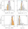 |
Fig. 2. Distributions of global stellar mass (a) and SFR (b); and local luminosity-weighted stellar metallicity (c) and galactocentric distances (d) normalized by the host effective radius for the 61 host and SNAs (gray shaded histogram and density plot), respectively. The corresponding median of each distribution is shown (gray dashed line). The three example galaxies from Fig. 1 are also highlighted (circles). The vertical orange region indicates the galactocentric distance of the Sun with respect to the reff of the MW (±1σ) around the best estimate (orange dashed line). |
Even though the global properties explored above have restricted the type of galaxies in which SNA are likely to be found, local properties have the potential to unveil the environmental physics of such regions. The local conditions of the SN have been widely studied in recent years and we have revealed a clear picture of our vicinity through a wide variety of stellar tracers (e.g., Bonatto & Bica 2011; Sollima 2019; Şahin & Bilir 2020; Whitten et al. 2021; Gontcharov & Mosenkov 2021, to name a few). The SN is known to be in an expanding local under-density called the local bubble (< 200 pc) with little to no star formation within (e.g., Zucker et al. 2022), low dust extinction (e.g., Gaia Collaboration 2018b), stellar metallicity around the solar value (e.g., Hayden et al. 2020), and an average (mass-weighted) stellar age ⟨log t/yr⟩M⋆ ∼ 9.5 (e.g., Reid et al. 2007). Outside this vicinity (< 1 kpc), solar neighborhood star formation takes place at a rate per square parsec of log Σψ⋆ ∼ −8.24 ± 0.09 M⊙ yr−1 pc−2. This yields a light dominant stellar component with an age ⟨log t/yr⟩L⋆ ≲ 9.38 ± 0.09 and metallicity ⟨[Z/Z⊙]⟩L⋆ ≲ − 0.08 ± 0.18 (Fig. 2c); with a surface mass density log ΣM⋆ ∼ 1.76 ± 0.07 M⊙ pc−2 and mass-to-light ratio in the V-band  (Flynn et al. 2006); and that is affected by a typical visual dust extinction AV ∼ 0.19 ± 0.02 mag.
In most of the cases, we find astonishing agreement in their local properties, despite the different methodologies adopted to derive the SNA values (stellar population synthesis of unresolved stars) and the SN ones (exploring the properties of resolved stellar populations; see e.g., Reid et al. 2007; Hayden et al. 2020; Gontcharov & Mosenkov 2021; Lacerda et al. 2022). Of the compared properties, we find a difference above 2σ for only the M⋆/L⋆ ratio, a parameter that is particularly difficult to derive for resolved stellar populations (e.g., Flynn et al. 2006).
As indicated before, we find that most of the SNA regions are located following a ring-like distribution around the galactic nucleus (e.g., Fig. 1). This ring seems to be located at different galactocentric distances for each galaxy, as suggested by Prantzos (2008) for the MW. We have noted above that this distance seemingly scales with the size of the galaxy. In order to check for this possibility, we present in Fig. 2d the distribution of the galactocentric distances for the SNAs normalized by the effective radius of the host galaxy. The fact that the SNA distance distribution can be characterized by a typical value is evidence that such regions tend to thrive around a typical scaled radii value, albeit with a significant scatter, σrSNA ∼ 1.79 reff. According to our estimates of the MW effective radius, the SN is located at a scaled galactocentric distance of rSN ∼ 1.95 ± 0.19 reff, assuming an absolute Sun galactocentric distance ∼8.2 ± 0.1 kpc (BH16). Interestingly, the median distance of SNAs and that of the Sun are ∼2, and they are apart by ∼0.1 reff.
4. Discussion and conclusions
Most of the efforts to characterize the GHZ in the MW are based on simulations of galaxy formation and chemical evolution. Lineweaver et al. (2004) simulated the physical conditions to produce a MW-like galaxy. They predicted that the Sun lies well within a locus of GHZ, which encompasses a stellar population with an age ≲4 − 8 Gyr (log t/yr ≲ 9.6 − 9.9) and galactocentric distances within ∼5 − 11 kpc (1.19 − 2.62 reff). Spitoni et al. (2014, 2017) developed chemical evolution simulations of the MW and M31 to predict the probability of finding terrestrial planets with the conditions to harbor life. In agreement with Lineweaver et al. (2004), they also found that Earth-like planets are more likely in the present than in the past, peaking near 8 kpc in galactocentric distance. Interestingly, Spitoni et al. (2014) found for M31 that Earth-like planets are prone to be found at systematically larger galactocentric radii ∼16 kpc. Similarly, Carigi et al. (2013) found ∼12–14 kpc for the same galaxy. Assuming a reff ∼ 9 kpc for M31, these radii are within 1σ of our distribution in Fig. 2d. These results are also consistent with earlier characterizations of the GHZ in our galaxy made by Lineweaver et al. (2004) and Prantzos (2008). They argued that, as the Galactic disk evolves inside out, the ring-shaped GHZ spreads toward inner and outer regions of the MW. The picture drawn from these simulations is consistent with our findings that the SNAs in galaxies other than the MW follow a ring-like structure, whose radii depends on the size of the galaxy. Consequently, the GHZ (as sampled by our SN definition) should be related to the timescale at which these galaxies are currently evolving, as gathered from their current total stellar mass and metallicity, SFR, etc.
In summary, the newly introduced methodology has allowed us to find SNAs using a nonparametric method. Most of the local properties of those regions and the global ones of their hosts agree with those of the SN and the MW. Furthermore, SNAs are found in a ring at a galactoentric distance that scales with the size of the galaxy. This result agrees with both our current understanding of the evolution of the stellar populations in galaxies (e.g., Sánchez 2020) and simulations predicting the optical location of both the GHZ and the presence of terrestrial planets. A study of the structural evolution of these potential GHZs at higher redshifts is in order.
We will analyze interacting galaxies in a another paper.
Acknowledgments
We thank the support by the PAPIIT-DGAPA grant AG100622. AMN thanks the support from the DGAPA-UNAM postdoctoral fellowship. LC thanks support from (PAPIIT-DGAPA, UNAM), grant IN-103820. JBB acknowledges support from the grant IA-101522 (PAPIIT-DGAPA, UNAM) and funding from the CONACYT grant CF19-39578. We thank the anonymous referee for his/her helpful comments. This study makes uses of the data provided by the Calar Alto Legacy Integral Field Area (CALIFA) survey (http://califa.caha.es). CALIFA is the first legacy survey being performed at Calar Alto. The CALIFA collaboration would like to thank the IAA-CSIC and MPIA-MPG as major partners of the observatory, and CAHA itself, for the unique access to telescope time and support in manpower and infrastructures. The CALIFA collaboration thanks also the CAHA staff for the dedication to this project. Funding for the Sloan Digital Sky Survey IV has been provided by the Alfred P. Sloan Foundation, the U.S. Department of Energy Office of Science, and the Participating Institutions. SDSS-IV acknowledges support and resources from the Center for High Performance Computing at the University of Utah. The SDSS website is www.sdss.org. SDSS-IV is managed by the Astrophysical Research Consortium for the Participating Institutions of the SDSS Collaboration including the Brazilian Participation Group, the Carnegie Institution for Science, Carnegie Mellon University, Center for Astrophysics, Harvard & Smithsonian, the Chilean Participation Group, the French Participation Group, Instituto de Astrofísica de Canarias, The Johns Hopkins University, Kavli Institute for the Physics and Mathematics of the Universe (IPMU)/University of Tokyo, the Korean Participation Group, Lawrence Berkeley National Laboratory, Leibniz Institut für Astrophysik Potsdam (AIP), Max-Planck-Institut für Astronomie (MPIA Heidelberg), Max-Planck-Institut für Astrophysik (MPA Garching), Max-Planck-Institut für Extraterrestrische Physik (MPE), National Astronomical Observatories of China, New Mexico State University, New York University, University of Notre Dame, Observatário Nacional/MCTI, The Ohio State University, Pennsylvania State University, Shanghai Astronomical Observatory, United Kingdom Participation Group, Universidad Nacional Autónoma de México, University of Arizona, University of Colorado Boulder, University of Oxford, University of Portsmouth, University of Utah, University of Virginia, University of Washington, University of Wisconsin, Vanderbilt University, and Yale University.
References
- Alzate, J. A., Bruzual, G., & Díaz-González, D. J. 2021, MNRAS, 501, 302 [Google Scholar]
- Aniyan, S., Freeman, K. C., Gerhard, O. E., Arnaboldi, M., & Flynn, C. 2016, MNRAS, 456, 1484 [CrossRef] [Google Scholar]
- Barrera-Ballesteros, J. K., Heckman, T., Sánchez, S. F., et al. 2021, ApJ, 909, 131 [NASA ADS] [CrossRef] [Google Scholar]
- Bland-Hawthorn, J., & Gerhard, O. 2016, ARA&A, 54, 529 [Google Scholar]
- Boardman, N., Zasowski, G., Seth, A., et al. 2020, MNRAS, 491, 3672 [NASA ADS] [CrossRef] [Google Scholar]
- Bonatto, C., & Bica, E. 2011, MNRAS, 415, 2827 [NASA ADS] [CrossRef] [Google Scholar]
- Buder, S., Lind, K., Ness, M. K., et al. 2019, A&A, 624, A19 [NASA ADS] [CrossRef] [EDP Sciences] [Google Scholar]
- Bundy, K., Bershady, M. A., Law, D. R., et al. 2015, ApJ, 798, 7 [Google Scholar]
- Cardelli, J. A., Clayton, G. C., & Mathis, J. S. 1989, ApJ, 345, 245 [Google Scholar]
- Carigi, L., García-Rojas, J., & Meneses-Goytia, S. 2013, Rev. Mex. Astron. Astrofis, 49, 253 [Google Scholar]
- De Silva, G. M., Freeman, K. C., Bland-Hawthorn, J., et al. 2015, MNRAS, 449, 2604 [NASA ADS] [CrossRef] [Google Scholar]
- Ding, P. J., Zhu, Z., & Liu, J. C. 2019, AJ, 158, 247 [NASA ADS] [CrossRef] [Google Scholar]
- Drory, N., MacDonald, N., Bershady, M. A., et al. 2015, AJ, 149, 77 [CrossRef] [Google Scholar]
- Espinosa-Ponce, C., Sánchez, S. F., Morisset, C., et al. 2022, MNRAS, 512, 3436 [NASA ADS] [CrossRef] [Google Scholar]
- Evans, D. W., Riello, M., De Angeli, F., et al. 2018, A&A, 616, A4 [NASA ADS] [CrossRef] [EDP Sciences] [Google Scholar]
- Flynn, C., Holmberg, J., Portinari, L., Fuchs, B., & Jahreiß, H. 2006, MNRAS, 372, 1149 [NASA ADS] [CrossRef] [Google Scholar]
- Forgan, D., Dayal, P., Cockell, C., & Libeskind, N. 2017, Int. J. Astrobiol., 16, 60 [NASA ADS] [CrossRef] [Google Scholar]
- Fraser-McKelvie, A., Merrifield, M., & Aragón-Salamanca, A. 2019, MNRAS, 489, 5030 [CrossRef] [Google Scholar]
- Gaia Collaboration (Brown, A. G. A., et al.) 2018a, A&A, 616, A1 [NASA ADS] [CrossRef] [EDP Sciences] [Google Scholar]
- Gaia Collaboration (Babusiaux, C., et al.) 2018b, A&A, 616, A10 [NASA ADS] [CrossRef] [EDP Sciences] [Google Scholar]
- Galbany, L., Anderson, J. P., Sánchez, S. F., et al. 2018, ApJ, 855, 107 [Google Scholar]
- Gobat, R., & Hong, S. E. 2016, A&A, 592, A96 [NASA ADS] [CrossRef] [EDP Sciences] [Google Scholar]
- Gontcharov, G. A., & Mosenkov, A. V. 2021, MNRAS, 500, 2590 [Google Scholar]
- Gonzalez, G., Brownlee, D., & Ward, P. 2001, Icarus, 152, 185 [Google Scholar]
- Gowanlock, M. G., Patton, D. R., & McConnell, S. M. 2011, Astrobiology, 11, 855 [NASA ADS] [CrossRef] [Google Scholar]
- Hayden, M. R., Bland-Hawthorn, J., Sharma, S., et al. 2020, MNRAS, 493, 2952 [Google Scholar]
- Helmi, A., Babusiaux, C., Koppelman, H. H., et al. 2018, Nature, 563, 85 [Google Scholar]
- Holtzman, J. A., Shetrone, M., Johnson, J. A., et al. 2015, AJ, 150, 148 [Google Scholar]
- Ibarra-Medel, H. J., Avila-Reese, V., Sánchez, S. F., González-Samaniego, A., & Rodríguez-Puebla, A. 2019, MNRAS, 483, 4525 [NASA ADS] [CrossRef] [Google Scholar]
- Lacerda, E. A. D., Sánchez, S. F., Cid Fernandes, R., et al. 2020, MNRAS, 492, 3073 [Google Scholar]
- Lacerda, E. A. D., Sánchez, S. F., Mejía-Narváez, A., et al. 2022, ArXiv e-prints [arXiv:2202.08027] [Google Scholar]
- Lineweaver, C. H., Fenner, Y., & Gibson, B. K. 2004, Science, 303, 59 [NASA ADS] [CrossRef] [Google Scholar]
- López-Cobá, C., Sánchez, S. F., Anderson, J. P., et al. 2020, AJ, 159, 167 [Google Scholar]
- Mejía-Narváez, A., Sánchez, S. F., Lacerda, E. A. D., et al. 2020, MNRAS, 499, 4838 [CrossRef] [Google Scholar]
- Mejía-Narváez, A., Bruzual, G., Sánchez, S. F., et al. 2021, ApJS, accepted [arXiv:2108.01697] [Google Scholar]
- Prantzos, N. 2008, Space Sci. Rev., 135, 313 [NASA ADS] [CrossRef] [Google Scholar]
- Prantzos, N., Abia, C., Limongi, M., Chieffi, A., & Cristallo, S. 2018, MNRAS, 476, 3432 [Google Scholar]
- Raymond, S. N., Izidoro, A., & Morbidelli, A. 2020, in Planetary Astrobiology, eds. V. S. Meadows, G. N. Arney, B. E. Schmidt, & D. J. Des Marais, 287 [Google Scholar]
- Reid, I. N., Turner, E. L., Turnbull, M. C., Mountain, M., & Valenti, J. A. 2007, ApJ, 665, 767 [NASA ADS] [CrossRef] [Google Scholar]
- Rodríguez-Puebla, A., Primack, J. R., Avila-Reese, V., & Faber, S. M. 2017, MNRAS, 470, 651 [Google Scholar]
- Ruiz-Lara, T., Gallart, C., Bernard, E. J., & Cassisi, S. 2020, Nat. Astron., 4, 965 [NASA ADS] [CrossRef] [Google Scholar]
- Şahin, T., & Bilir, S. 2020, ApJ, 899, 41 [CrossRef] [Google Scholar]
- Sánchez, S. F. 2020, ARA&A, 58, 99 [Google Scholar]
- Sánchez, S. F., Kennicutt, R. C., Gil de Paz, A., et al. 2012, A&A, 538, A8 [Google Scholar]
- Sánchez, S. F., Rosales-Ortega, F. F., Iglesias-Páramo, J., et al. 2014, A&A, 563, A49 [CrossRef] [EDP Sciences] [Google Scholar]
- Sánchez, S. F., Pérez, E., Sánchez-Blázquez, P., et al. 2016a, Rev. Mex. Astron. Astrofis., 52, 171 [Google Scholar]
- Sánchez, S. F., Pérez, E., Sánchez-Blázquez, P., et al. 2016b, Rev. Mex. Astron. Astrofis., 52, 21 [NASA ADS] [Google Scholar]
- Sánchez, S. F., Avila-Reese, V., Rodríguez-Puebla, A., et al. 2019, MNRAS, 482, 1557 [Google Scholar]
- Sánchez, S. F., Walcher, C. J., Lopez-Cobá, C., et al. 2021, Rev. Mex. Astron. Astrofis., 57, 3 [Google Scholar]
- Sollima, A. 2019, MNRAS, 489, 2377 [NASA ADS] [CrossRef] [Google Scholar]
- Spitoni, E., Matteucci, F., & Sozzetti, A. 2014, MNRAS, 440, 2588 [NASA ADS] [CrossRef] [Google Scholar]
- Spitoni, E., Gioannini, L., & Matteucci, F. 2017, A&A, 605, A38 [NASA ADS] [CrossRef] [EDP Sciences] [Google Scholar]
- Valerdi, M., Barrera-Ballesteros, J. K., Sánchez, S. F., et al. 2021, MNRAS, 505, 5460 [NASA ADS] [CrossRef] [Google Scholar]
- Vergely, J. L., Ferrero, R. F., Egret, D., & Koeppen, J. 1998, A&A, 340, 543 [NASA ADS] [Google Scholar]
- Vukotić, B., Steinhauser, D., Martinez-Aviles, G., et al. 2016, MNRAS, 459, 3512 [Google Scholar]
- Walcher, C. J., Wisotzki, L., Bekeraité, S., et al. 2014, A&A, 569, A1 [NASA ADS] [CrossRef] [EDP Sciences] [Google Scholar]
- Wall, J. V., & Jenkins, C. R. 2003, Practical Statistics for Astronomers, Cambridge Observing Handbooks for Research Astronomers (Cambridge University Press) [Google Scholar]
- Whitten, D. D., Placco, V. M., Beers, T. C., et al. 2021, ApJ, 912, 147 [NASA ADS] [CrossRef] [Google Scholar]
- Yan, R., Chen, Y., Lazarz, D., et al. 2019, ApJ, 883, 175 [Google Scholar]
- Yanny, B., Rockosi, C., Newberg, H. J., et al. 2009, AJ, 137, 4377 [Google Scholar]
- Zackrisson, E., Calissendorff, P., González, J., et al. 2016, ApJ, 833, 214 [NASA ADS] [CrossRef] [Google Scholar]
- Zucker, C., Goodman, A. A., Alves, J., et al. 2022, Nature, 601, 334 [NASA ADS] [CrossRef] [Google Scholar]
All Tables
Median global and local properties for the MW and the SN, respectively, compared to the SNA hosts’ and regions’ values retrieved in this Letter.
All Figures
|
Fig. 1. Demonstration of our method for finding SNAs with three sample galaxies in our golden sample. Top panels: RGB (R: 6450 Å, G: 5375 Å, and B: 3835 Å) composite images of galaxies NGC 5947, NGC 5000, and NGC 309 in our golden sample described in Sect. 2.3 which likely hosts SNA regions. The likelihood map is overlaid in each case with contours enclosing the 1σ (solid), 2σ (dashed), and 3σ (dotted), respectively. The location of the maximum likelihood in each case (colored circle) and its galactocentric distance (dashed colored line) are shown. Bottom panel: spectrum corresponding to the maximum likelihood spaxel (solid line in color) along with the propagated (1σ) error spectrum (shaded region). We highlight the regions where the error spectrum was masked out (dotted). The SNA spectrum (gray) calculated as described in Sect. 2.4 is also shown. The resulting χ2 and the likelihood integrated within a circular aperture matching the SN physical scale around the maximum are also shown. |
| In the text | |
|
Fig. 2. Distributions of global stellar mass (a) and SFR (b); and local luminosity-weighted stellar metallicity (c) and galactocentric distances (d) normalized by the host effective radius for the 61 host and SNAs (gray shaded histogram and density plot), respectively. The corresponding median of each distribution is shown (gray dashed line). The three example galaxies from Fig. 1 are also highlighted (circles). The vertical orange region indicates the galactocentric distance of the Sun with respect to the reff of the MW (±1σ) around the best estimate (orange dashed line). |
| In the text | |
Current usage metrics show cumulative count of Article Views (full-text article views including HTML views, PDF and ePub downloads, according to the available data) and Abstracts Views on Vision4Press platform.
Data correspond to usage on the plateform after 2015. The current usage metrics is available 48-96 hours after online publication and is updated daily on week days.
Initial download of the metrics may take a while.