© ESO 2022

1. Introduction

Magnetohydrodynamic (MHD) waves are a ubiquitous phenomenon in the solar atmosphere. Observation of waves in the corona (Schrijver et al. 1999; Aschwanden et al. 1999; Nakariakov et al. 1999; Tomczyk et al. 2007), chromosphere (De Pontieu et al. 2007; Morton et al. 2012; Verth & Jess 2016), and photosphere (Dorotovič et al. 2008; Fujimura & Tsuneta 2009; Grant et al. 2015; Moreels et al. 2015; Keys et al. 2018; Gilchrist-Millar et al. 2021) allows both solar atmospheric seismology and the study of the coronal heating problem.

Inference of plasma parameters by matching observed oscillations with theoretical results has been done for the solar corona (Nakariakov et al. 1999; Nakariakov & Ofman 2001; Nakariakov & Verwichte 2005; Aschwanden et al. 2003; Goossens et al. 2008; Andries et al. 2005; Van Doorsselaere et al. 2011) and the photosphere (Fujimura & Tsuneta 2009; Moreels & Van Doorsselaere 2013). Coronal structures such as loops and filament threads in particular are also known to harbor MHD waves which contribute to the heating of the corona (Parnell & De Moortel 2012; Arregui 2015; Nakariakov et al. 2016; Nakariakov & Kolotkov 2020; Van Doorsselaere et al. 2020). More recently, observations in a photospheric pore of propagating slow surface sausage modes reported by Grant et al. (2015) were damped over a sufficiently short length scale to be able to heat the chromosphere, suggesting waves in structures of the lower atmosphere are relevant to this problem as well. The energy carried by the oscillations can be partially conveyed to the background plasma through various processes such as phase mixing, resonant absorption (Zaitsev & Stepanov 1975; Hollweg & Yang 1988; Hollweg et al. 1990; Goossens et al. 1992, 2002; Cadez et al. 1997; Erdélyi et al. 2001; Soler et al. 2009, 2013; Yu et al. 2017), mode coupling (Pascoe et al. 2010, 2012; Hollweg et al. 2013; De Moortel et al. 2016), and the development of turbulence by the Kelvin-Helmholtz instability (Heyvaerts & Priest 1983; Ofman et al. 1994; Karpen et al. 1994; Karampelas et al. 2017; Afanasyev et al. 2019; Hillier et al. 2020; Shi et al. 2021; Geeraerts & Van Doorsselaere 2021).

When studying them theoretically through an analytical model, solar atmospheric structures such as coronal loops, filament threads, sunspots, and photospheric pores are often modeled as a straight cylinder with a circular base in a first approximation. Roberts & Webb (1979), Wentzel (1979), Spruit (1982), and Edwin & Roberts (1983), among others, discussed cylinder modes in ideal MHD analytically for the case where the structure has a discontinuous boundary. However, this assumption of a discontinuous separation between two homogeneous plasmas inside and outside the cylinder is a very crude approximation of reality. Indeed, the introduction of an inhomogeneous boundary layer gives rise to new physics, among which the process of resonant absorption. With the emergence of two continua in the spectrum of ideal MHD, namely the Alfvén and cusp continua, new local oscillations called continuum modes come into existence. These localized modes can be excited by either externally driven waves or a discrete eigenmode of the cylinder that couples to them, in a process called resonant absorption. In the case of an eigenmode being resonantly absorbed, it is damped because of its energy being transferred to local Alfvén or slow waves within the boundary layer. This happens at the position where the frequency of the eigenmode is equal to one of the continuum frequencies.

In the eigenvalue problem of linearized ideal MHD, where one assumes the waves to be normal modes of the system, the frequency of a discrete mode that is resonantly absorbed is complex because of the damping. However, the ideal MHD force operator being self-adjoint (Goedbloed & Poedts 2004), its eigenvalues must be real and hence the resonantly absorbed discrete mode is no longer an eigenmode. Instead, it becomes a so-called quasimode (also called a virtual eigenmode or a collective mode), which is the response of a system being excited at one of its natural frequencies and being damped because of its energy being transferred to a continuum mode. It is a dominant, global, exponentially decaying response to an initial perturbation (Tirry & Goossens 1996), which cannot be distinguished from a true eigenmode over timescales that are much smaller than the damping time of the mode; this has been discussed in detail for example by Sedláček (1971), Zhu & Kivelson (1988), and Goedbloed & Poedts (2004) in different contexts. The efficiency of a quasimode in transferring heat to the surrounding plasma has been ascertained in works such as Poedts et al. (1989), Poedts & Kerner (1991), Tirry & Goossens (1996), De Groof & Goossens (2000), and Goossens & De Groof (2001).

When resistivity is added in the model, the singularities in the differential equations giving rise to the continua disappear and the continuum modes become discrete eigenmodes instead (Goedbloed et al. 2010). The quasimode also becomes a true eigenmode now, as was discussed by Poedts & Kerner (1991). Its damping is then stronger due to both resonant absorption and resistivity. The quasimode frequency is recovered in the limit of vanishing resistivity. The present study focuses on quasimodes with the oscillatory part of their frequency within the cusp continuum, and so photospheric conditions are of particular interest, because in a cylinder with a discontinuous boundary, the slow surface mode has its frequency within the interval that becomes the cusp continuum when an inhomogeneous layer is included (Edwin & Roberts 1983). The efficiency of damping due to resonant absorption of the slow surface mode in the cusp continuum compared to purely resistive damping was studied by Chen et al. (2018) for the sausage mode and Chen et al. (2021) for the kink mode, both in photospheric conditions. Their results suggest electrical resistivity is more efficient overall by about an order of magnitude, although damping due to resonant absorption of the slow surface kink mode in the cusp continuum dominates both damping due to resonant absorption in the Alfvén continuum and resistive damping at the lower end of the relevant values of resistivity.

In this paper, we work out an analytical method to find the dispersion relation of modes in a cylinder with an inhomogeneous layer of arbitrary width separating two homogeneous regions inside and outside. The method follows the work of Soler et al. (2013), who used Frobenius series around the Alfvén resonant position to represent the solution of the eigenfunctions in the inhomogeneous layer. These latter authors assume the plasma to be pressureless, making the cusp continuum disappear from the system, and focus on kink modes resonantly absorbed in the Alfvén continuum in coronal conditions. The aim of the present study is to extend their method to a plasma where thermal pressure is included, and to focus rather on slow surface modes resonantly absorbed in the cusp continuum. The results not only allow us to understand the damping of the resulting quasimode and compare it to the numerical resistive results of Chen et al. (2018), but also to study the behavior of the quasimode perturbations around the cusp resonant point. Additionally, the method can be used to plot the eigenfunctions of continuum modes.

2. Model

We consider a cylindrical solar atmospheric flux tube with a circular cross-section and an inhomogeneous transition layer at the boundary that separates two regions of homogeneous plasma with different properties (see Fig. 1). Although modes in photospheric structures such as pores and sunspots are the main focus of this paper, the method we outline here can be repeated under different conditions.

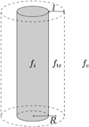Fig. 1. Sketch of the model cylinder. Quantities assume a constant value fi inside, a possibly different constant value fe outside, and have a continuously varying profile ftr linking the two through the inhomogeneous layer. The radius of the cylinder is denoted R and the layer width is denoted l.

In this model, we work in the framework of linearized ideal MHD, and cylindrical coordinates (r, ϕ, z) are used. The main physical quantities of interest are mass density, plasma velocity, magnetic field, and thermal pressure, respectively denoted ρ, v, B, and p. For a quantity f, its linearized form is written f₀ + f₁, where f₀ stands for the background part and f₁ for the first-order perturbation. We assume that there is no background velocity (v₀ = 0), and that the background magnetic field is aligned with the axis of the cylinder, as the pores and sunspots we have in mind typically have strong axial magnetic fields which act as a waveguide. We therefore take B₀ = B_0z1_z. As the background quantities are independent of φ, z, and t, the perturbed quantities can be Fourier-analyzed as $f_1={\stackrel{\sim }{f}}_1(r)exp\left\{i(n\phi +k_{z}z-\omega t)\right\}$. In what follows, we drop the tilde and use f₁ to refer to ${\stackrel{\sim }{f}}_1$ for any quantity f.

The background quantities are assumed constant in both the internal and external regions, although the values are assumed to be possibly different in both regions. In the inhomogeneous layer at the boundary of the cylinder, that is to say for r ∈ [R − l/2, R + l/2] with R the cylinder radius and l the layer width, the quantities are assumed to vary continuously in r and to follow a predefined profile. It should be noted that, in reality, the profiles for the variation of the quantities are unknown and one therefore has to make an arbitrary assumption about them in analytical models.

From the previously cited quantities, one can define the Lagrangian plasma displacement ξ from v = D_m(ξ) (with D_m denoting the material derivative), which is equal to $\frac{\partial \mathit{\xi }}{\partial t}$ in the linear case without background velocity, and the perturbed total pressure P₁ as $P_1=p_1+\frac{{\mathit{B}}_0·{\mathit{B}}_1}{{\mathrm{\mu }}_0}$ (i.e., the sum of the perturbed thermal and magnetic pressures), with μ₀ being the magnetic permeability of free space. Following Appert et al. (1974), the ideal MHD quantities can be reduced to two coupled first-order ordinary differential equations (ODE) for ξ_r and P₁ under the assumptions previously mentioned:

$$\begin{array}{cc}& D\frac{\mathrm{d}}{\mathrm{d}r}\left(r{\xi }_r\right)=-C_{1}r{P}_1\text{,}\hfill \end{array}$$(1)

$$\begin{array}{cc}& D\frac{\mathrm{d}{P}_1}{\mathrm{d}r}=C_2{\xi }_r\text{,}\hfill \end{array}$$(2)

where

$$\begin{array}{cc}& D=\rho (v_{\mathrm{A}}^2+v_{\mathrm{s}}^2)({\omega }^2-{\omega }_{\mathrm{A}}^2)({\omega }^2-{\omega }_{\mathrm{C}}^2)\text{,}\hfill \end{array}$$(3)

$$\begin{array}{cc}& C_1={\omega }^4-(v_{\mathrm{A}}^2+v_{\mathrm{s}}^2)\left({\displaystyle \frac{n^2}{r^2}+k_z^2}\right)({\omega }^2-{\omega }_{\mathrm{C}}^2)\text{,}\hfill \end{array}$$(4)

$$\begin{array}{cc}& C_2={\rho }_0^2(v_{\mathrm{A}}^2+v_{\mathrm{s}}^2){({\omega }^2-{\omega }_{\mathrm{A}}^2)}^2({\omega }^2-{\omega }_{\mathrm{C}}^2)\text{,}\hfill \end{array}$$(5)

and with $v_{\mathrm{A}}=B_{0z}/\sqrt{{\mathrm{\mu }}_0{\rho }_0}$ the Alfvén speed, $v_{\mathrm{s}}=\sqrt{\gamma p_0/{\rho }_0}$ the sound speed, $v_{\mathrm{C}}=v_{\mathrm{A}}{v}_{\mathrm{s}}/(v_{\mathrm{A}}^2+v_{\mathrm{s}}^2{)}^{1/2}$ the cusp speed, ω_A = k_zv_A the Alfvén frequency, and ω_C = k_zv_C the cusp frequency. Equations (1) and (2) can be combined into a single second-order ODE for P₁:

$$\begin{array}{c}\hfill \frac{{\mathrm{d}}^2{P}_1}{r^2}+\{\frac{1}{r}-\frac{\frac{\mathrm{d}}{\mathrm{d}r}\left[{\rho }_0({\omega }^2-{\omega }_{\mathrm{A}}^2)\right]}{{\rho }_0({\omega }^2-{\omega }_{\mathrm{A}}^2)}\}\frac{\mathrm{d}{P}_1}{\mathrm{d}r}+(-m^2-\frac{n^2}{r^2})P_1=0\text{,}\end{array}$$(6)

where

$$\begin{array}{c}\hfill m=\sqrt{{\displaystyle \frac{({\omega }_{\mathrm{A}}^2-{\omega }^2)({\omega }_{\mathrm{s}}^2-{\omega }^2)}{({\omega }_{\mathrm{C}}^2-{\omega }^2)(v_{\mathrm{A}}^2+v_{\mathrm{s}}^2)}}}\text{,}\end{array}$$(7)

and with ω_s = k_zv_s the sound frequency. Here, $\sqrt{z}$ of a number z ∈ ℂ is meant to be the solution w ∈ ℂ to z = w² with $-\frac{\pi }{2}<\text{Arg}(\mathit{w})\le \frac{\pi }{2}$. Then, from Eq. (2), the expression for ξ_r can be derived once P₁ is known:

$$\begin{array}{c}\hfill {\displaystyle {\xi }_r=\frac{1}{{\rho }_0({\omega }^2-{\omega }_{\mathrm{A}}^2)}\frac{\mathrm{d}{P}_1}{\mathrm{d}r}\text{.}}\end{array}$$(8)

3. Finding the solutions for P₁ and ξ_r

In this section, we seek a solution for P₁ from Eq. (6). Knowing the solution of P₁, one can determine the solution of ξ_r from Eq. (8). The solutions for the other quantities can then be derived from P₁ and ξ_r. There are three regions where different solution forms will occur: inside the cylinder, in the inhomogeneous layer, and outside the cylinder.

3.1. Solutions in the internal and external regions

In the homogeneous plasmas of the internal (i.e., where r <  R − l/2) and external (i.e., where r >  R + l/2) regions, Eq. (6) will simplify because all background quantities are constant. Indeed, the ODE for P₁ will reduce to

$$\begin{array}{c}\hfill {\displaystyle \frac{{\mathrm{d}}^2{P}_1}{r^2}+\frac{1}{r}\frac{\mathrm{d}{P}_1}{\mathrm{d}r}+(-m^2-\frac{n^2}{r^2})P_1=0\text{.}}\end{array}$$(9)

This is a Bessel equation, the solution of which is well known and can be found for example in Edwin & Roberts (1983). For surface modes, the internal solution P_1i and the external solution P_1e are then

$$\begin{array}{cc}& P_{1i}=C_1{I}_n(m_{i}r)\text{,}\hfill \end{array}$$(10)

$$\begin{array}{cc}& P_{1e}=C_2{K}_n(m_{e}r)\text{,}\hfill \end{array}$$(11)

where I_n is the modified Bessel function of the first kind of order n, K_n is the modified Bessel function of the second kind of order n, and m_i and m_e are the versions of m in respectively the internal and external regions, whereas C₁ and C₂ are constants. In what follows, we need the solutions for ξ_r as well, which are obtained from Eq. (8) and are given as follows for the internal and external regions:

$$\begin{array}{cc}& {\displaystyle {\xi }_{\mathit{ri}}=\frac{C_1{m}_i}{{\rho }_{0i}({\omega }^2-{\omega }_{\mathit{Ai}}^2)}{I}_n^{\prime }(m_{i}r)\text{,}}\hfill \end{array}$$(12)

$$\begin{array}{cc}& {\displaystyle {\xi }_{\mathit{re}}=\frac{C_2{m}_e}{{\rho }_{0e}({\omega }^2-{\omega }_{\mathit{Ae}}^2)}{K}_n^{\prime }(m_{e}r)\text{.}}\hfill \end{array}$$(13)

3.2. Solutions in the inhomogeneous layer

In the inhomogeneous boundary layer, the background quantities are not constant and vary continuously from their value inside the cylinder to their value in the surrounding plasma. Therefore, the full ODE for P₁, Eq. (6), needs to be solved. The radial variation of the background quantities in the boundary layer, specifically v_A and v_C, gives rise to singularities of the ODE (6) at positions r_A and r_C which respectively satisfy ${\omega }^2={\omega }_{\mathrm{A}}^2(r_{\mathrm{A}})$ and ${\omega }^2={\omega }_{\mathrm{C}}^2(r_{\mathrm{C}})$. These singularities are both regular singular points of the ODE and were discussed by Sakurai et al. (1991) in the limit of a thin layer (i.e., l/R ≪ 1) where they were assumed to be real. In what follows, we assume that $v_{\mathrm{A}}^2$ and $v_{\mathrm{C}}^2$ are strictly monotonic functions of r.

To solve Eq. (6), we work out a method based on that developed by Soler et al. (2013). The authors of that paper use Frobenius series solutions around the Alfvén resonant point in order to represent the solution of P₁ inside the layer. However, with the inclusion of a cusp resonance point, complications arise compared to the case discussed by Soler et al. (2013). Indeed, because of the presence of both Alfvén and cusp resonance, there will now be two singularities arising within the inhomogeneous layer. A Frobenius series around one of the resonant points will have its convergence radius limited because of the presence of the other resonant point nearby, and vice versa. This means the whole layer will not be covered by the convergence disk of a single series when both resonant points are present. In addition, depending on the transition profiles chosen for the background quantities in the inhomogeneous layer, additional singularities of the coefficients in the ODE (6) may be present near the layer and also have an impact on the convergence radii of the series. We therefore need to make multiple series expansions: around the cusp resonant position (r_C), the Alfvén resonant position (r_A), and some regular points of Eq. (6) until a whole path linking the points R − l/2 and R + l/2 in the complex r-plane is covered by convergence disks.

3.2.1. Frobenius solution around r_C

The resonant position r_C being a regular singular point of the ODE (6) as well (Sakurai et al. 1991), we write a solution locally around r_C as a Frobenius series:

$$\begin{array}{c}\hfill {\displaystyle P_1(r)={\displaystyle \sum _{k=0}^{\infty }}{p}_k{(r-r_{\mathrm{C}})}^{k+s}\text{.}}\end{array}$$(14)

By inserting this solution into the equation, one finds the indicial equation. Sakurai et al. (1991) showed that this equation is s(s − 1)=0 for a strictly monotonic transition profile of $v_{\mathrm{A}}^2$. Hence two basic independent solutions of Eq. (6) are

$$\begin{array}{cc}& {\displaystyle P_{1,1,\mathrm{C}}(r)={\displaystyle \sum _{k=0}^{\infty }}{\alpha }_k{(r-r_{\mathrm{C}})}^{k+1}\text{,}}\hfill \end{array}$$(15)

$$\begin{array}{cc}& {\displaystyle P_{1,2,\mathrm{C}}(r)={\displaystyle \sum _{k=0}^{\infty }}{\sigma }_k{(r-r_{\mathrm{C}})}^k+{\mathcal{C}}_{\mathrm{C}}{P}_{1,1,\mathrm{C}}(r-r_{\mathrm{C}})ln(r-r_{\mathrm{C}})\text{,}}\hfill \end{array}$$(16)

where the coefficients α₀ and σ₀ can both be freely chosen because of the two degrees of freedom in the general solution of a second-order ODE, whereas the remaining α_k and σ_k, as well as the constant 𝒞_C, are determined by recursion relations (see Appendix A). Hereafter, α₀ and σ₀ are both taken equal to 1. The logarithm in the solution (16) appears because of the cusp resonance, which is clarified below. The general solution is therefore given by

$$\begin{array}{c}\hfill P_1(r)=A_1{P}_{1,1,C}(r)+A_2{P}_{1,2,C}(r)\end{array}$$(17)

within the convergence radius of the two involved power series, with A₁ and A₂ being some arbitrary coefficients.

The expression for the quantity 𝒞_C in Eq. (16) is determined by the recursion relation for the coefficients σ_k and is useful further below; in Appendix B, we show that it is given by

$$\begin{array}{c}\hfill {\displaystyle {\mathcal{C}}_{\mathrm{C}}=-\frac{k_z^4{v}_{\mathrm{C}}^4(r_{\mathrm{C}})}{(v_{\mathrm{A}}^2(r_{\mathrm{C}})+v_{\mathrm{s}}^2(r_{\mathrm{C}}))\frac{\mathrm{d}{\omega }_{\mathrm{C}}^2}{\mathrm{d}\zeta }{|}_{r=r_{\mathrm{C}}}}\text{.}}\end{array}$$(18)

3.2.2. Frobenius solution around r_A

For the solution of Eq. (6) in the form of a Frobenius series around the Alfvén resonant position r_A, we proceed similarly by inserting

$$\begin{array}{c}\hfill {\displaystyle P_1(r)={\displaystyle \sum _{k=0}^{\infty }}{p}_k{(r-r_{\mathrm{A}})}^{k+s}}\end{array}$$(19)

into the ODE. The obtained indicial equation in this case is s(s − 2)=0, as was also derived by Sakurai et al. (1991) for a strictly monotonic transition profile of $v_{\mathrm{A}}^2$. Hence, two independent basic solutions are

$$\begin{array}{cc}& {\displaystyle P_{1,1,\mathrm{A}}(r)={\displaystyle \sum _{k=0}^{\infty }}{\beta }_k{(r-r_{\mathrm{A}})}^{k+2}\text{,}}\hfill \end{array}$$(20)

$$\begin{array}{cc}& {\displaystyle P_{1,2,\mathrm{A}}(r)={\displaystyle \sum _{k=0}^{\infty }}{\tau }_k{(r-r_{\mathrm{A}})}^k+{\mathcal{C}}_{\mathrm{A}}{P}_{1,1,\mathrm{A}}(r-r_{\mathrm{A}})ln(r-r_{\mathrm{A}})\text{,}}\hfill \end{array}$$(21)

where the coefficients β₀ and τ₀ are chosen freely, whereas the remaining β_k and τ_k as well as the constant 𝒞_A are determined by recursion relations (see Appendix A). Hereafter, β₀ and τ₀ are both taken equal to 1 as well. The logarithm in the solution (21) appears because of the Alfvén resonance, which is also clarified below. The general solution is then given by

$$\begin{array}{c}\hfill P_1(r)=A_3{P}_{1,1,A}(r)+A_4{P}_{1,2,A}(r)\end{array}$$(22)

within the convergence radius of the two involved power series, with A₃ and A₄ some arbitrary coefficients. The value of the quantity 𝒞_A is determined by the recursive relation for the τ_k.

3.2.3. Power series solution around regular points

The power series solution around a regular point r₀ of the ODE (6) can be found by inserting a general power series of the form

$$\begin{array}{c}\hfill {\displaystyle P_1(r)={\displaystyle \sum _{k=0}^{\infty }}{p}_k{(r-r_0)}^k}\end{array}$$(23)

in Eq. (6). The two first coefficients can be chosen freely, yielding the two basic solutions

$$\begin{array}{cc}& {\displaystyle P_{1,1,r_0}(r)={\displaystyle \sum _{k=0}^{\infty }}{a}_k{(r-r_0)}^k\text{,}}\hfill \end{array}$$(24)

$$\begin{array}{cc}& {\displaystyle P_{1,2,r_0}(r)={\displaystyle \sum _{k=0}^{\infty }}{b}_k{(r-r_0)}^k\text{,}}\hfill \end{array}$$(25)

which are independent if the couples (a₀, a₁) and (b₀, b₁) are not multiples of one another. The remaining a_k and b_k are again determined by a recursion relation (see Appendix A). The general solution is then given by

$$\begin{array}{c}\hfill P_1(r)=A_{r_0}{P}_{1,1,r_0}(r)+B_{r_0}{P}_{1,2,r_0}(r)\end{array}$$(26)

within the convergence radius of the two involved power series, with A_r0 and B_r0 being some arbitrary coefficients.

4. Constructing the dispersion relation

To find the eigenmodes and quasimodes of the system, one needs to find a dispersion relation which expresses the frequency ω as a function of the wavenumbers k_z and n. To achieve this, boundary conditions need to be imposed at the positions r_i = R − l/2 and r_e = R + l/2 where the internal and external solutions are linked with the solution in the inhomogeneous layer.

In order to satisfy the boundary conditions at the points r_i and r_e, we need to connect them with a path that is fully covered by convergence disks of series expansions around points in the complex r-plane (see Fig. 2), following a process called analytic continuation. The effects of both the cusp and the Alfvén resonances need to be taken into account, so both r_C and r_A must lie on the path. We choose the path such that the coefficients of Eq. (6) are analytic in all other points composing it, so that we can locally represent the solution of the ODE as a regular power series around those points. In order to do this, we first identify the singularities of the coefficients of Eq. (6). These depend on the transition profiles chosen for the background quantities in the inhomogeneous layer. It is assumed that r_i and r_e are analytic points of the coefficients of Eq. (6), as is the case in the example discussed in Sect. 5.

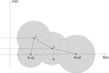Fig. 2. Representation of a path (thick solid line) linking ri = R − l/2 with re = R + l/2, formed by the line segments [rirC], [rCrA], and [rAre]. The dashed lines represent branch cuts due to the presence of the logarithms in the Frobenius solutions. In this representation, the represented disks only have radii of 80% of those of the corresponding convergence disks, as this was used in numerical calculations to avoid inaccuracy due to the slow convergence of the series near the edges of the convergence disks.

As can be seen from the Frobenius solutions in the previous section, both r_C and r_A are logarithmic branch points. The path may in principle not cross branch cuts, as the series expansions would then be defining P₁ on the next Riemann sheet. Theoretically, it would be sufficient to make the path circumvent a branch point and its branch cut, but in practice we find that, in some situations, substantial numerical accuracy is lost in this way due to the need for (1) a high number of expansion points and (2) convergence disks with a very small radius. Instead, we always choose the shortest path, and, when needing to cross a branch cut, we correct for the jump at the last encountered branch point.

4.1. Nonoverlapping cusp and Alfvén continua

Sakurai et al. (1991) derived connection formulae for both P₁ and ξ_r across the cusp resonant layer in the thin boundary (TB) limit (i.e., l/R ≪ 1). In the case where the cusp and Alfvén continua are not overlapping, these can be used to derive the dispersion relation for modes that undergo resonant absorption in the cusp continuum. This situation was discussed for example by Yu et al. (2017), who derived the corresponding dispersion relation in that limit (see Eq. (27) therein). That dispersion relation can be recovered from our model, as we show below.

4.1.1. General dispersion relation

If we assume that the cusp and Alfvén continua do not overlap, then only one resonant point will be present at a time. To find a dispersion relation in this particular case, we compute the series expansions of two basic independent solutions P_1, 1 and P_1, 2 of the ODE (6) along a path in the complex r-plane which links r_i with r_e and includes r_C. Such solutions are defined over a subset of ℂ, but are locally represented by a power series (if expanding around a regular point) or a Frobenius solution (if expanding around a regular singular point). The two basic solutions P_1, 1 and P_1, 2 we choose are the ones that are locally represented respectively by the Frobenius solutions P_1, 1, C and P_1, 2, C from Eqs. (15) and (16), with α₀ = σ₀ = 1 within the convergence disk of the involved power series. For each of the two solutions P_1, 1 and P_1, 2, we then find the local representation as a power series or Frobenius solution around a new point on the path and within the convergence disk of the former local representation, and so on until we cover the whole path.

For this, we use the following result: two power series $\sum _{k=0}^{\infty }{f}_k{(r-r_1)}^k$ and $\sum _{k=0}^{\infty }{g}_k{(r-r_2)}^k$ are equal on the overlapping region between their respective convergence disks if

$$\begin{array}{c}\hfill {\displaystyle g_k={\displaystyle \sum _{j=k}^{\infty }}{f}_j\left(\begin{array}{c}j\\ k\end{array}\right){(r_2-r_1)}^{j-k}\text{.}}\end{array}$$(27)

We therefore calculate the first two coefficients of the new power series expansion with formula (27), and compute the remaining ones from the recursion relation for the series expansion (23) around a regular point.

Once we have series representations for the complex functions P_1, 1 and P_1, 2 along the whole path, we can compute P_1, 1(r_i), P_1, 1(r_e), P_1, 2(r_i), and P_1, 2(r_e). Using [f]_i and [f]_e to denote the jumps of a quantity f across respectively the ends r_i and r_e of the inhomogeneous layer, we impose the following four boundary conditions which need to be satisfied for physical reasons:

$$\begin{array}{c}\hfill {[P_1]}_i=0,{[P_1]}_e=0,{[{\xi }_r]}_i=0,{[{\xi }_r]}_e=0\text{.}\end{array}$$(28)

Introducing the notations

$$\begin{array}{cc}& {\mathcal{G}}_{i,e}=P_{1,1}(r_{i,e})\hfill \end{array}$$(29)

$$\begin{array}{cc}& {\mathcal{F}}_{i,e}=P_{1,2}(r_{i,e})\hfill \end{array}$$(30)

$$\begin{array}{cc}& {\displaystyle {\mathrm{\Xi }}_{i,e}=\frac{1}{{\rho }_0(r_{i,e})({\omega }^2-{\omega }_A^2(r_{i,e}))}\frac{\mathrm{d}{P}_{1,1}}{\mathrm{d}r}(r_{i,e})}\hfill \end{array}$$(31)

$$\begin{array}{cc}& {\displaystyle {\mathrm{\Gamma }}_{i,e}=\frac{1}{{\rho }_0(r_{i,e})({\omega }^2-{\omega }_A^2(r_{i,e}))}\frac{\mathrm{d}{P}_{1,2}}{\mathrm{d}r}(r_{i,e})\text{,}}\hfill \end{array}$$(32)

we can then rewrite Eq. (28) as

$$\begin{array}{cc}\hfill C_1{I}_n(m_i{r}_i)& =C_3{\mathcal{G}}_i+C_4{\mathcal{F}}_i\text{,}\hfill \end{array}$$(33)

$$\begin{array}{cc}\hfill C_2{K}_n(m_e{r}_e)& =C_3{\mathcal{G}}_e+C_4{\mathcal{F}}_e\text{,}\hfill \end{array}$$(34)

$$\begin{array}{cc}\hfill {\displaystyle \frac{C_1{m}_i}{{\rho }_{0i}({\omega }^2-{\omega }_{\mathit{Ai}}^2)}{I}_n^{\prime }(m_i{r}_i)}& =C_3{\mathrm{\Xi }}_i+C_4{\mathrm{\Gamma }}_i\text{,}\hfill \end{array}$$(35)

$$\begin{array}{cc}\hfill {\displaystyle \frac{C_2{m}_e}{{\rho }_{0e}({\omega }^2-{\omega }_{\mathit{Ae}}^2)}{K}_n^{\prime }(m_e{r}_e)}& =C_3{\mathrm{\Xi }}_e+C_4{\mathrm{\Gamma }}_e\text{.}\hfill \end{array}$$(36)

Equations (33)–(36) form a system of four equations in the four unknowns C₁, C₂, C₃, and C₄. In order to have a nontrivial solution, the determinant of this system needs to vanish. This yields the following dispersion relation:

$$\begin{array}{c}\hfill {\displaystyle \frac{\frac{m_e}{{\rho }_{0e}({\omega }^2-{\omega }_{\mathit{Ae}}^2)}\frac{K_n^{\prime }(m_e{r}_e)}{K_n(m_e{r}_e)}{\mathcal{G}}_e-{\mathrm{\Xi }}_e}{\frac{m_e}{{\rho }_{0e}({\omega }^2-{\omega }_{\mathit{Ae}}^2)}\frac{K_n^{\prime }(m_e{r}_e)}{K_n(m_e{r}_e)}{\mathcal{F}}_e-{\mathrm{\Gamma }}_e}-\frac{\frac{m_i}{{\rho }_{0i}({\omega }^2-{\omega }_{\mathit{Ai}}^2)}\frac{I_n^{\prime }(m_i{r}_i)}{I_n(m_i{r}_i)}{\mathcal{G}}_i-{\mathrm{\Xi }}_i}{\frac{m_i}{{\rho }_{0i}({\omega }^2-{\omega }_{\mathit{Ai}}^2)}\frac{I_n^{\prime }(m_i{r}_i)}{I_n(m_i{r}_i)}{\mathcal{F}}_i-{\mathrm{\Gamma }}_i}=0\text{.}}\end{array}$$(37)

Hereafter, the left-hand side of this equation is referred to as the dispersion function. It is multivalued because of the logarithm ln(r − r_C) in P_1, 2, and so one needs to choose where to lay the branch cut. We take it to lie on the negative real axis of r − r_C, in which case the branch cuts of the dispersion function lie exactly on the cusp continuum when viewed as a function of ω. The reason for making this choice is explained below.

4.1.2. Thin boundary limit

In the TB limit, that is to say when l/R ≪ 1, the dispersion relation (37) can be approximated. In order to do so, we note that in this limit r ≈ r_C for every r within the inhomogeneous layer because it is narrow. We therefore make the approximation that r_C ≈ R. The series expansions in Eqs. (15), (16), (24), and (25) can then be approximated by only including the zeroth-order terms of the respective series expansions, yielding the following approximations:

$$\begin{array}{cc}& {\mathcal{G}}_{i,e}\approx 0\text{,}\hfill \end{array}$$(38)

$$\begin{array}{cc}& {\mathcal{F}}_{i,e}\approx 1\text{,}\hfill \end{array}$$(39)

$$\begin{array}{cc}& {\displaystyle {\mathrm{\Xi }}_{i,e}\approx \frac{1}{{\rho }_0(R)({\omega }_{\mathrm{C}}^2(R)-{\omega }_A^2(R))}\text{,}}\hfill \end{array}$$(40)

$$\begin{array}{cc}& {\mathrm{\Gamma }}_{i,e}\approx \frac{{\mathcal{C}}_{\mathrm{C}}(1+ln(\mp l/2))}{{\rho }_0(R)({\omega }_{\mathrm{C}}^2(R)-{\omega }_A^2(R))}\text{.}\hfill \end{array}$$(41)

Then, making the approximations m_er_e ≈ m_eR and m_ir_i ≈ m_iR in the arguments of the modified Bessel functions, and using the expression for 𝒞_C derived in Eq. (18), the dispersion relation (37) is approximated by

$$\begin{array}{cc}\hfill {\displaystyle \frac{m_e}{{\rho }_{0e}({\omega }^2-{\omega }_{\mathit{Ae}}^2)}\frac{K_n^{\prime }(m_{e}R)}{K_n(m_{e}R)}-}& \frac{m_i}{{\rho }_{0i}({\omega }^2-{\omega }_{\mathit{Ai}}^2)}\frac{I_n^{\prime }(m_{i}R)}{I_n(m_{i}R)}\hfill \\ \hfill & =-\frac{\pi v_{\mathrm{C}}^4(R)ln(-1)}{{\rho }_0(R)v_{\mathrm{A}}^4(R)\frac{\mathrm{d}{v}_{\mathrm{C}}^2}{\mathrm{d}r}{|}_{r=R}}\text{.}\hfill \end{array}$$(42)

Here, ln(−1) must be chosen as either iπ or −iπ such that the frequency of the mode has a negative imaginary part (corresponding to a damped mode). Equation (42) is equivalent to the dispersion relation derived by Yu et al. (2017) in the thin boundary limit.

4.2. Overlapping cusp and Alfvén continua

In some situations, such as the photospheric conditions of Edwin & Roberts (1983), the value of the equilibrium quantities are such that the cusp and Alfvén continua overlap. For n ≠ 0, this has the effect of introducing an Alfvén resonant position along with the cusp resonant position in the inhomogeneous layer. The sausage modes (n = 0) are not resonantly absorbed in the Alfvén continuum in this model (Sakurai et al. 1991), and hence for them there is only the resonant position r_C.

The method that we outlined in the previous section is useful for finding the general expression (37) for the dispersion relation, allowing us to recover the analytical approximation for nonoverlapping continua in the thin boundary limit from Yu et al. (2017). However, solving the dispersion relation in the general case needs to be done numerically, which is not done efficiently with this method. We also note that Soler et al. (2009) found an analytical thin boundary approximation to the dispersion relation for overlapping continua based on the individual jumps at the Alfvén and cusp resonant positions derived by Sakurai et al. (1991). This relation will not be recovered here.

First, we encounter an additional difficulty when the cusp and Alfvén continua are overlapping. Indeed, when trying to find local representations of the basic solutions P_1, 1 and P_1, 2 as either power series or Frobenius solutions, the Alfvén resonant position needs to be included on the path linking r_i with r_e along which we seek these representations. When making the calculations, we find that the presence of the nonzero constant 𝒞_A when n ≠ 0 prevents us from using the method outlined above. Second, we lose some accuracy with every new expansion point included in the path to analytically continue each of the two solutions P_1, 1 and P_1, 2. Some accuracy is lost for two reasons: (1) every series needs to be truncated; and (2) the first two coefficients of the series in every new local representation are approximations themselves due to the fact that the series in formula (27) need to be truncated as well. In addition, each new expansion point increases the computational cost of the numerical algorithm to create and solve the dispersion relation. This means that we need to minimize the number of local representations of a solution to the ODE (6) in order to maximize efficiency in the numerical computations.

A more practical method, which reduces both the number of local representations of solutions and the loss in accuracy in the computation of each representation, consists of covering the path with local representations of unrelated general solutions and linking them together with additional boundary conditions. The values of the first free coefficients in a series determine a specific solution. In the former method, we started from a specific solution and calculated the local representations of that solution along a path. We did this independently for two solutions, namely the one represented in a region around r_C by the Frobenius solution (15) with coefficient α₀ = 1 and the one represented in a region around r_C by the Frobenius solution (16) with coefficients σ₀ = 1 and α₀ = 1. For each new local representation, we thus needed to compute the corresponding values of the first free coefficients. The two solutions, being independent, together form a general solution (17) in the inhomogeneous layer. We then linked this general solution with the solutions outside the homogeneous layer through the boundary conditions (28). In the following method, we instead compute local representations of general solutions of the form (17), (22), or (26), with coefficients α₀ = 1 and σ₀ = 1 in the case of a Frobenius solution (17), β₀ = 1 and τ₀ = 1 in the case of a Frobenius solution (22), and (a₀, a₁)=(1, 0) and (b₀, b₁)=(0, 1) in the case of a power series solution (26). This we do along a path in the complex r-plane which links r_i with r_e, includes both r_C and r_A, and is entirely covered by convergence disks around expansion points.

Each of these local representations then includes two arbitrary constants. On each region where the convergence disks of two neighboring general solutions overlap, we equate the general solutions of P₁ and ξ_r. This determines two out of the four involved constants. With N expansion points covering the path, there are 2N arbitrary constants involved. Equating neighboring general solutions of both P₁ and ξ_r on every overlapping region between pairs of convergence disks yields 2N − 2 equations. This means 2N − 2 of the arbitrary constants can be written as a function of two remaining ones, which we refer to as C₃ and C₄. These two constants C₃ and C₄, which are related to the solution in the inhomogeneous layer, then, together with the two constants C₁ and C₂ related to the solutions in the homogeneous regions respectively inside and outside the cylinder, yield a system of four equations in the four unknowns C₁, C₂, C₃, and C₄ when we impose the four boundary conditions (28). For the obtained system to have nontrivial solutions, its 4 × 4 determinant must be equal to zero. This determinant, when viewed as a function of the complex variable ω, is called the dispersion function. Equating the dispersion function to zero forms the dispersion relation, which needs to be solved numerically. We chose to use this method, rather than the one outlined in the previous section, in order to find the modes in the general case.

We note that the dispersion function is multivalued because of both ln(r − r_C) and ln(r − r_A); for general n, it has two branch points r_C and r_A in the complex r-plane, and hence also two branch cuts (see Fig. 2). These branch cuts are arbitrary from a mathematical point of view, but from a physical standpoint they have to be taken such that the principal Riemann sheet of the dispersion function does not have complex zeros. The reason for this is explained in the following section. We find that taking the branch cuts of both ln(r − r_C) and ln(r − r_A) to lie on the negative real axis of their respective arguments ensures that there are no complex zeros on the principal Riemann sheet of the dispersion function. Viewed in the complex ω domain, the branch cuts of the dispersion function then correspond exactly to the cusp and Alfvén continua on the real axis. This also means that, in the case where the continua overlap, the two branch cuts also overlap. A path that crosses this overlapping region will then continue on one of two possible Riemann sheets.

5. Frequency and perturbation profiles of the quasimode in photospheric conditions

5.1. Theoretical considerations

In this section, we apply the methods outlined in the previous section to the specific case of a cylindrical structure in the photosphere, for example a pore or a sunspot. For this, we take (v_Ae, v_si, v_se)=(1/4, 1/2, 3/4)v_Ai, corresponding to the photospheric conditions in Fig. 3 of Edwin & Roberts (1983).

The existence of an inhomogeneous boundary layer results in the possibility for continuum modes with a frequency in the cusp continuum [ω_Ce, ω_Ci] to be excited. In the absence of a layer, the slow surface mode has its frequency in that interval as well, and so it is natural to expect this mode to couple to a local cusp continuum mode with the same frequency if a layer is present. The damping it undergoes because of the transfer of its energy to the continuum mode is then expected to be expressed in the fact that the imaginary part of its frequency becomes strictly negative, with the frequency thus becoming complex.

However, it is a proven result that the ideal MHD operator is Hermitian and can therefore only have real eigenfrequencies (Goedbloed & Poedts 2004). Our dispersion relation being satisfied for some value ω₀ of the frequency is equivalent to finding a zero of the dispersion function at ω₀ on its principal Riemann sheet. Therefore, no complex zero of the dispersion function should be found on that sheet. We ensure this by taking the branch cuts in the way we define them in the previous section.

The proper study of a quasimode, being a natural oscillatory response to an initial perturbation, needs to be done by solving the initial value problem with the Laplace transform. The quasimode is then found as a pole of a (multivalued) Green’s function, namely as a zero on the neighboring Riemann sheet of its denominator. This denominator is the dispersion function. The contribution of that pole is then taken into account when computing the inverse Laplace transform, by deforming the Bromwich contour across the branch cut (which is the continuum) onto the next Riemann sheet.

The method we developed as part of the study presented here solves the eigenvalue problem by considering normal modes and constructing the dispersion function for eigenmodes from the physical considerations expressed in the boundary conditions (28). The quasimode, not being an eigenmode, therefore does not naturally appear when solving this problem. However, as the dispersion function has the same zeros as the one in the initial value problem, one can find the frequencies of quasimodes by looking on its next Riemann sheet. The quasimode frequency ω₀ that we find there does not satisfy the dispersion relation, because on the principal Riemann sheet ω₀ is not a zero of the dispersion function. This means that a quasimode perturbation cannot be continuous in the two boundaries of the inhomogeneous layer and at the resonant position at the same time. Furthermore, in order to access another Riemann sheet of the dispersion function, a different branch of the logarithm in the large Frobenius solution around a resonant position r_res must be used on each side of the line r = Re[r_res]. This ensures the discontinuity occurs at the resonant position rather than at one of the boundaries of the layer, which is the only physically acceptable solution.

The aim of our method is to find the values of the complex frequency of the quasimode corresponding to the slow surface mode of the discontinuous boundary case in photospheric conditions in order to quantify its damping. In particular, we would like to know the profile of the damping time as a function of the layer width l for values of the longitudinal wavenumber k_z that are realistic for oscillations in photospheric pores. It is also interesting to plot the profiles of the quasimode perturbations, and compare them for different values of l and k_z.

5.2. Result for an example case

The dispersion function obviously depends on the transition profiles of the background quantities in the inhomogeneous layer. Theoretically, any profile could be taken. However, in the specific example we are now going to work out, we choose relatively simple transition profiles in order for the numerical calculations to remain feasible: we assume the squared cusp and squared sound speeds to have a linear profile in the layer. These in turn fix the profiles of the square Alfvén speed, magnetic field, thermal pressure, and density.

The linear profiles for the squared cusp and squared sound speeds in the inhomogeneous layer are taken as follows:

$$\begin{array}{cc}& v_{\mathrm{C}}^2(r)=\stackrel{\sim }{v_{\mathrm{C}}^2}r+\widehat{v_{\mathrm{C}}^2}\text{,}\hfill \end{array}$$(43)

$$\begin{array}{cc}& v_{\mathrm{s}}^2(r)=\stackrel{\sim }{v_{\mathrm{s}}^2}r+\widehat{v_{\mathrm{s}}^2}\text{,}\hfill \end{array}$$(44)

with the constants defined as

$$\begin{array}{cc}& {\displaystyle \stackrel{\sim }{v_{\mathrm{C}}^2}=\frac{v_{\mathrm{C}e}^2-v_{\mathrm{C}i}^2}{l}\text{,}}\hfill \end{array}$$(45)

$$\begin{array}{cc}& {\displaystyle \stackrel{\sim }{v_{\mathrm{s}}^2}=\frac{v_{\mathrm{s}e}^2-v_{\mathrm{s}i}^2}{l}\text{,}}\hfill \end{array}$$(46)

$$\begin{array}{cc}& \widehat{v_{\mathrm{C}}^2}=\left({\displaystyle \frac{1}{2}+\frac{R}{l}}\right)v_{\mathrm{C}i}^2+\left({\displaystyle \frac{1}{2}-\frac{R}{l}}\right)v_{\mathrm{C}e}^2\text{,}\hfill \end{array}$$(47)

$$\begin{array}{cc}& \widehat{v_{\mathrm{s}}^2}=\left({\displaystyle \frac{1}{2}+\frac{R}{l}}\right)v_{\mathrm{s}i}^2+\left({\displaystyle \frac{1}{2}-\frac{R}{l}}\right)v_{\mathrm{s}e}^2\text{.}\hfill \end{array}$$(48)

With these profiles, we can now try to find the quasimode that corresponds to the slow surface eigenmode in the discontinuous boundary case as a complex zero of the dispersion function on its first Riemann sheet neighboring the principal sheet.

5.2.1. Sausage mode

For the sausage mode, the case is simplified as there is only one branch point r_C in the complex r-plane. The quasimode frequencies ω obtained with our series method, normalized with respect to the internal cusp frequency ω_Ci, are shown as functions of l/R in Fig. 3 (real part) and Fig. 4 (imaginary part) for k_zR = 1, k_zR = 3, and k_zR = 5. These values for the longitudinal wavenumber correspond to those observed in slow sausage modes in photoshperic pores by Grant et al. (2015), for which k_z ∈ [1, 5]. Figure 4 also contains the imaginary part of the quasimode frequency calculated with the dispersion relation in the thin boundary approximation (42).

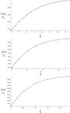Fig. 3. Real part of the frequency of the slow sausage quasimode (solid line) as a function of l/R for kzR = 1 (top), kzR = 3 (middle), and kzR = 5 (bottom). The hollow circles represent the quasimode, with the frequency calculated from the dispersion relation obtained through the series method outlined in the previous sections. The full circle is the frequency of the slow surface sausage mode in the case of a discontinuous boundary, calculated from the dispersion relation in Edwin & Roberts (1983) under the same physical conditions.

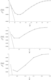Fig. 4. Imaginary part of the frequency of the slow sausage quasimode (solid line) as a function of l/R for kzR = 1 (top), kzR = 3 (middle), and kzR = 5 (bottom) calculated from the dispersion relation obtained through the series method outlined in the previous sections. The modes represented here are the same as those from Fig. 3. The dashed line is the imaginary part of the frequency of the slow sausage quasimode calculated with the thin boundary approximation (42).

In Fig. 3, we notice that the quasimode frequency approaches the internal cusp frequency in its real part as l/R is increased. This can also be seen in Fig. 4 in Chen et al. (2018), which is produced from numerical computations in the resistive MHD model and shows the real part of the resistive eigenfrequency of the slow sausage mode as a function of l/R in the same physical setup although with slightly different transition profiles. This is not taken into account in the analytical thin boundary (TB) approximation, where the oscillatory part of the frequency is assumed constant (Yu et al. 2017).

The imaginary parts of the quasimodes, in Fig. 4, display a behavior which might be unexpected. Initially, as l/R is slightly increased, the imaginary part is increased in absolute value as well, corresponding to a stronger damping. However, after some critical value of l/R – which depends on k_zR – has been reached, the absolute value of the imaginary part of the quasimode becomes smaller again and stays on this decreasing path. This stands in contrast with both the thin tube thin boundary (TTTB) approximation for nonaxisymmetric modes and the TB approximation for the slow surface mode, as the damping is found to monotonically increase with l/R in those cases. In Fig. 4, we can indeed see that the imaginary part of the frequency agrees very well with the result from the TB approximation when l/R → 0, but that the two diverge from a certain value of l/R onward as the TB estimation continues to increase indefinitely in absolute value.

The nonmonotonic behavior in the imaginary part of the frequency was also found for fast kink quasimodes in the Alfvén continuum in the cold plasma case for certain transition profiles by Soler et al. (2013), although for other profiles it is absent. It therefore appears that the presence of this behavior depends on the transition profiles. Yu & Van Doorsselaere (2019) also find that mode conversion in coronal loops is more efficient when the transition layer is thin, as long as the transition profile is approximately linear at the resonant position.

As l/R is increased, the quasimode frequency comes very close to the internal cusp frequency ω_Ci. For values of l/R above a certain critical value, which is about 0.75 for k_zR = 1, 0.40 for k_zR = 3, and 0.25 for k_zR = 1, the discussed series method no longer allows us to properly compute the quasimode frequency. The frequency ω_Ci is a pole of the dispersion function as well as an accumulation point for the slow body modes that are not resonantly absorbed on the other side, making it impossible on a practical level to distinguish the quasimode from the pole and the infinite number of slow body modes in a sufficiently small region around ω_Ci. It is therefore not clear whether the frequency of the quasimode goes to the internal cusp frequency as a limit point when l/R is increased, or goes past the internal cusp frequency and leaves the cusp continuum in its real part, where it would still be within the Alfvén continuum, which overlaps with part of the cusp continuum in the present photospheric conditions. However, as sausage modes are not resonantly absorbed in the Alfvén continuum in the present model (Sakurai et al. 1991), if a complex frequency were to be found outside the cusp continuum for these higher values of l/R it should probably be discarded as only a mathematical continuation that no longer has physical sense, because there would be no continuum modes for the slow sausage mode to couple to.

We can also look at the ratio of the damping time τ = 1/|Im[ω]| to the period T = 2π/|Re[ω]| of the quasimode. This is shown in Fig. 5, where τ/T is plotted as a function of l/R for the three different values of k_zR considered before. The lowest value we find for τ/T is about 300 at l/R = 0.05 and k_zR = 5. This is larger than the damping time-to-period ratio of the resistive slow surface sausage eigenmode studied by Chen et al. (2018), who found a τ/T ≈ 100 for k_zR = 4.3 and τ/T ≈ 200 for k_zR = 2, at l/R = 0.1. This higher damping in the resistive case is to be expected of course, as resistivity provides an extra damping mechanism on top of resonant absorption. The graph of τ/T provided by these latter authors also exhibits a convex shape, which can clearly be seen in our Fig. 5 for k_zR = 1 in our case too. As was also shown by Chen et al. (2018) through the TB dispersion relation obtained by Yu et al. (2017) and which we recovered in Eq. (42) with our model, the analytical TB approximation does not yield this convex structure and it overestimates the damping as l/R is increased. This also confirms our finding that, at least for some transition profiles in the inhomogeneous layer, the damping of the mode does not monotonically increase as the transition layer width l/R increases.

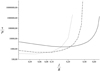Fig. 5. Damping time-to-period ratio τ/T as a function of l/R, for kzR = 1 (solid line), kzR = 3 (dashed line), and kzR = 5 (dotted line). Both axes of the plot are in logarithmic scale.

We see that the ideal results for slow sausage modes in the cusp continuum derived in this paper provide a relatively good match to the resistive results from Chen et al. (2018). This also confirms independently what Chen et al. (2018) concluded from their numerical study in resistive MHD, namely that the efficiency of resonant absorption of slow surface sausage modes in the cusp continuum in photospheric conditions is relatively low and that other processes such as resistive damping might be more efficient for those modes.

We can also look at the profiles of the perturbations of the quasimode. The profiles of P₁, ξ_r, and ξ_z for a layer width of l/R = 0.1 are shown in Fig. 6 (for k_zR = 1), Fig. 7 (for k_zR = 3), and Fig. 8 (for k_zR = 5). As the singularity of Eq. (6) lies in the complex plane, the solutions of this ODE are complex as well. This can be seen in the figures. We also notice that ξ_z peaks at the resonant position near the left boundary of the layer, and is much larger than ξ_r at the same position. This is to be expected, as Sakurai et al. (1991) showed that for modes that are resonantly absorbed in the cusp continuum the dominant contribution in the perturbations comes from ξ_z.

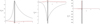Fig. 6. Real (black) and imaginary (red) parts of the quasimode perturbations P1, ξr, and ξz, with kzR = 1 and l/R = 0.1. The values of r are normalized to R. The linear transition profile defined by Eqs. (43)–(48) is taken in the inhomogeneous layer, which is represented in gray.

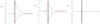Fig. 7. Real (black) and imaginary (red) parts of the quasimode perturbations P1, ξr, and ξz, with kzR = 3 and l/R = 0.1. The values of r are normalized to R. The linear transition profile defined by Eqs. (43)–(48) is taken in the inhomogeneous layer, which is represented in gray.

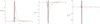Fig. 8. Real (black) and imaginary (red) parts of the quasimode perturbations P1, ξr, and ξz, with kzR = 5 and l/R = 0.1. The values of r are normalized to R. The linear transition profile defined by Eqs. (43)–(48) is taken in the inhomogeneous layer, which is represented in gray.

Figure 9 shows the perturbations P₁, ξ_r, and ξ_z for l/R = 0.75 and k_zR = 1. These are quite different in shape from the perturbations for l/R = 0.1, as is expected because the inhomogeneous layer is now much thicker. It was noted by Soler et al. (2013) that, because the singularity is not on the real axis, P₁ has a finite jump at the real part of the resonant position when plotting the profile over the positive real r-axis, even in the case of a thin layer. The jump conditions found in Sakurai et al. (1991), which state that P₁ does not jump in a thin layer, are therefore only approximately true. However, Soler et al. (2013) found that the jump is much larger for a much thicker layer. As can be seen in Fig. 9, this is not the case here as the jump in P₁ remains very small and is invisible in the figure. The reason for this is that, unlike in the case discussed by Soler et al. (2013), here the singularity stays close to the real axis (and actually approaches it) when l/R is increased from 0.1 to 0.75. This can be seen in Fig. 4.

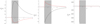Fig. 9. Real (black) and imaginary (red) parts of the quasimode perturbations P1, ξr, and ξz, with kzR = 1 and l/R = 0.75. The values of r are normalized to R. The linear transition profile defined by Eqs. (43)–(48) is taken in the inhomogeneous layer, which is represented in gray.

We also note that the resonant position is very close to the inner boundary of the inhomogeneous layer. This is to be expected, because in the case of a discontinuous boundary without a layer, the slow surface mode has its frequency just below the internal cusp frequency in the interval [ω_Ce, ω_Ci]. As we saw in Fig. 3, the introduction of an inhomogeneous boundary layer only slightly changes the real part of the frequency of this mode. In contrast to this, the resonant position of the kink modes resonantly absorbed in the Alfvén continuum is situated near the middle of the inhomogeneous layer, as was shown by Soler et al. (2013). We recover the same results about the position of the two resonances for continuum modes in Sect. 6.

5.2.2. Kink and fluting modes

For modes with n ≠ 0, the overlapping of the cusp and Alfvén continua produces two branch points in the complex r-plane and thus a double branch cut on the overlapping part of the two continua (which is exactly the cusp continuum here) in the complex ω-plane. This renders the problem considerably more difficult to solve.

Indeed, in the case of a single resonant point, the Riemann sheets can be denoted with a so-called sheetnumber, depending on which branch of the logarithm is considered. The principal Riemann sheet then corresponds to a sheetnumber of 0, whereas the neighboring sheets have sheetnumbers 1 and −1. In the theory for handling quasimodes with the Laplace transform method, as was laid out by both Sedláček (1971) and Goedbloed & Poedts (2004), the Bromwich contour is deformed in such a way that it surrounds the two zeros of the dispersion function which lie on the sheets with sheetnumbers 1 and −1 and have a negative imaginary part. These two zeros have an opposite oscillatory part of the frequency and an equal damping part, and represent a quasimode.

However, in the case of two resonant points, the introduction of the double branch cut on the cusp continuum implies that there are two dimensions in which a neighboring Riemann sheet can be considered. There are indeed two logarithms and hence in this case the sheets are denoted with a sheetcouple. The principal Riemann sheet is then denoted with the sheetcouple (0, 0), whereas there are eight neighboring Riemann sheets corresponding to the sheetcouples ( − 1, 1), (0, 1), (1, 1), ( − 1, 0), (1, 0), ( − 1, −1), (0, −1), and (1, −1). We found that, in this case, there are zeros on various Riemann sheets but not on all of them. In addition, the zeros are not symmetric as in the m = 0 case, in the sense that they neither have an opposite oscillatory part nor an equal imaginary part.

There would therefore be several zeros – with different values for ω – to consider when solving the Laplace transform in this situation, requiring us to somehow deform the Bromwich contour to all eight neighboring Riemann sheets. It is not clear how the Laplace transform method has to be adapted to this much more intricate situation; we do not know whether all zeros are physically relevant and represent quasimodes or not. If only one had to be considered, it is unclear why the others would have to be rejected. This situation is therefore not handled here, but could be an interesting subject for a future study.

6. Eigenfunctions of continuum modes

In the case of continuum modes, the frequency is real and the singularity lies on the real r-axis. As explained for example in Goedbloed & Poedts (2004), the large Frobenius solution (i.e., the one containing the logarithm) is continuous across the singularity, whereas the small Frobenius solution may jump. This implies that the general solution around a resonance point contains an additional arbitrary constant, which renders the system of equations formed by the boundary conditions inhomogeneous and thus allows them to always be fulfilled for continuum modes, independently of their frequency. Unlike for the quasimode, each basic independent solution of the ODE (6) is real for the continuum mode, because the singularity now lies on the real axis instead of in the complex plane. With real coefficients in the general solutions, the continuum eigenfunctions are therefore either real or imaginary, but not complex.

6.1. Sausage modes

We recall that, under the photospheric conditions (v_Ae, v_si, v_se)=(1/4, 1/2, 3/4)v_Ai assumed in the previous sections, the sausage mode is resonantly absorbed in the cusp continuum but not in the Alfvén continuum. The value of the additional arbitrary constant that arises from the resonant cusp position lying on the real r-axis then determines the amplitude of the perturbation.

In their Fig. 3, Goossens et al. (2021) plotted the modulus of the radial profile of some eigenfunctions of a resistive sausage eigenmode which corresponds to a continuum mode in ideal MHD, assuming a small resistivity and a sinusoidal transition profile in $v_{\mathrm{C}}^2$ and $v_{\mathrm{s}}^2$ in the inhomogeneous layer. We attempt to recover the eigenfunctions ξ_r and ξ_z from their figure by plotting the corresponding eigenfunctions of the continuum mode counterpart with our series method in ideal MHD. We assume the same resonant cusp position at about r = 0.955R, the same values of k_zR = 2, and l/R = 0.1, but we have a linear transition profile for $v_{\mathrm{C}}^2$ and $v_{\mathrm{s}}^2$ instead of a sinusoidal one.

The obtained eigenfunction profiles for perturbed total pressure P₁, radial displacement ξ_r, azimuthal displacement ξ_φ, and longitudinal displacement ξ_z are shown in Fig. 10. The eigenfunctions ξ_φ and ξ_z can be computed from P₁ and are defined as follows:

$$\begin{array}{cc}\hfill {\xi }_{\phi }& {\displaystyle =\frac{\mathit{in}}{\rho r({\omega }^2-{\omega }_{\mathrm{A}}^2)}{P}_1\text{,}}\hfill \end{array}$$(49)

$$\begin{array}{cc}\hfill {\xi }_z& {\displaystyle =\frac{i{k}_z{v}_{\mathrm{s}}^2}{\rho (v_{\mathrm{A}}^2+v_{\mathrm{s}}^2)({\omega }^2-{\omega }_{\mathrm{C}}^2)}{P}_1\text{.}}\hfill \end{array}$$(50)

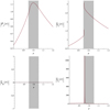Fig. 10. Moduli of the sausage continuum eigenfunctions P1, ξr, ξφ, and ξz, with rC = 0.955R, kzR = 2, and l/R = 0.1. The values of r are normalized to R. The linear transition profile defined by Eqs. (43)–(48) is taken in the inhomogeneous layer, which is represented in gray.

Our continuum eigenfunction for ξ_z matches the resistive eigenfunction of Goossens et al. (2021) relatively well, but less so for ξ_r. In Fig. 10, P₁ seems to have a sharp bend at r_C. However, from the expression of P₁ it can be verified that the graph is actually smooth and has a vertical tangent at that position, although it happens in a relatively small neighborhood around r_C. Consequently, the perturbation ξ_r, which is proportional to $\frac{\text{d}{P}_1}{\text{d}r}$ around r_C, seems to have a jump at this resonant position; in reality it has a vertical asymptote there, as both sides go to infinity. The difference between the ideal continuum eigenfunctions and the resistive eigenfunctions might be due to resistivity smoothing over the apparent bend of P₁ at r_C. The dominating perturbation at the cusp resonant position is ξ_z, in agreement with the analytical discussions by Sakurai et al. (1991) for example. As this is a sausage mode, ξ_φ is identically zero.

6.2. Kink modes

In the case of kink modes, resonant absorption occurs both in the cusp and Alfvén continua. For each frequency in the overlapping continua, a continuum mode will now have two singularities and thus two additional arbitrary constants, namely D_C at the cusp resonant position and D_A at the Alfvén resonant position. It is not entirely clear how these are related. As in the case of only one resonant position, the boundary conditions are fulfilled for every continuum frequency and the amplitude can be freely chosen. However, the inclusion of a second arbitrary constant entails that the radial profile itself differs in function of the ratio D_C/D_A.

The eigenfunctions P₁, ξ_r, ξ_φ, and ξ_z of the continuum mode obtained from our series method in ideal MHD and corresponding to the resistive kink eigenmode shown by Goossens et al. (2021) in their Figs. 1 and 2 are shown in Fig. 11. To compare our eigenfunctions with theirs, we assume the same resonant cusp position at about r = 0.955R, and the same values of k_zR = 0.7 and l/R = 0.1, but we have again a linear transition profile for $v_{\mathrm{C}}^2$ and $v_{\mathrm{s}}^2$ instead of a sinusoidal one. Here, we chose a ratio of D_C/D_A = 1, though a priori it seems any ratio would be acceptable as the boundary conditions are always fulfilled.

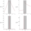Fig. 11. Moduli of the kink continuum eigenfunctions P1, ξr, ξφ and ξz, with rC = 0.955R, kzR = 0.7, and l/R = 0.1. The values of r are normalized to R. The linear transition profile defined by Eqs. (43)–(48) is taken in the inhomogeneous layer, which is represented in gray. The ratio between the two arbitrary constants DC and DA has been taken as equal to 1 here.

Our continuum eigenfunctions match the resistive eigenfunctions in Fig 1. of Goossens et al. (2021) relatively well, except for ξ_r. In Fig. 11, P₁ appears to have a sharp bend at r_C again, but looking at its analytical expression we see that its radial profile is actually smooth and the graph has a vertical tangent at that position. The difference with the resistive eigenfunctions might again be due to resistivity smoothing over regions where the ideal profile is sharper.

Around the Alvén resonant position r_A ≈ R, P₁ is visibly smooth on the plot, as can also be verified analytically. Indeed, ξ_r is not directly proportional to $\frac{\text{d}{P}_1}{\text{d}r}$ at this position because of the extra factor $1/({\omega }^2-{\omega }_{\mathrm{A}}^2)$ in its definition. The eigenfunction ξ_r has a vertical asymptote at r_A, whereas we have $\frac{\text{d}{P}_1}{\text{d}r}=0$ there.

Furthermore, the dominating perturbation is ξ_z at the cusp resonant position and ξ_φ at the Alfvén resonant position. This is again in agreement with the analytical derivations of Sakurai et al. (1991).

As a comparison with the setup in Fig. 11, we show the continuum eigenfunction of P₁ with a ratio D_C/D_A = 2 and D_C/D_A = 1/2 in Fig. 12. We see that the value of the ratio has an influence on the shape of the eigenfunction. It is not clear whether all ratios are physically acceptable or an additional constraint fixes the ratio to one possible value.

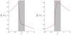Fig. 12. Modulus of the kink continuum eigenfunction P1 for ratios DC/DA = 2 (left) and DC/DA = 1/2 (right), with rC = 0.955R, kzR = 0.7, and l/R = 0.1. The values of r are normalized to R. The linear transition profile defined by Eqs. (43)–(48) is taken in the inhomogeneous layer, which is represented in gray.

7. Conclusion

In this study, we investigated the slow surface mode in a straight cylinder with a circular base with an inhomogeneous layer included at the boundary through the eigenvalue problem. We extended the Frobenius series method used by Soler et al. (2013) for a different mode and in a different model in order to adapt it to the situation where multiple series expansions are needed to cover the inhomogeneous layer. We were then able to find a dispersion relation for the eigenmodes of the cylinder. We first took the thin boundary limit of this relation and recovered the approximative dispersion relation in the thin boundary approximation found by Yu et al. (2017). Next, we investigated the full dispersion relation for a boundary layer of arbitrary width.

The inclusion of a finite inhomogeneous layer gives rise to the Alfvén and cusp continua in the frequency spectrum of the eigenmodes. A discrete mode having a frequency within one of these continua will then couple to a local continuum mode and become a damped global oscillation called a quasimode. Basing ourselves on the quasimode studies through the Laplace transform of Sedláček (1971) and Goedbloed & Poedts (2004) in order to find the quasimode from our dispersion function, we were able to find the complex frequency of the quasimode that corresponds to the slow surface mode of the discontinuous boundary case with its frequency in the cusp continuum.

We then proceeded to discuss an example case for the sausage mode, in which we took relatively simple transition profiles for the background MHD quantities in order for the analytical calculations to remain feasible. In resistive MHD, the quasimode becomes an eigenmode, and so we compared our analytical results for the slow sausage mode to the numerical results obtained by Chen et al. (2018) from resistive MHD computations under the same model and the same background conditions (although with different transition profiles). Our findings are in line with the results and conclusions of this latter paper. In particular, we find the profile of the damping time-to-period ratio for our quasimode, which is important for characterizing the damping of a mode by resonant absorption, to be similar both in shape and in scale to their resistive slow sausage eigenmode. The small difference in scale is explained by the fact that resistivity is an additional damping mechanism with respect to ideal MHD. We also discuss the quasimode perturbations, and find that the jump in P₁ at the resonant position remains small, unlike in the case of the kink quasimode resonantly absorbed in the Alfvén continuum in a cold plasma discussed by Soler et al. (2013).

The case of nonaxisymmetric quasimodes is not extensively discussed in the present paper. As the Alfvén and cusp continua overlap in the photospheric background conditions of interest in the present work, these modes will couple to continuum modes from both continua at the same time. As the effect this has on the frequency of the quasimode is not yet well understood, we only briefly mention that case. However, this could be a subject for further study.

We also used the series method to plot the perturbation profiles of the sausage and kink ideal continuum modes corresponding to the resistive eigenmodes of Goossens et al. (2021). We find that the continuum eigenfunctions match the resistive eigenfunctions relatively well, and propose that the difference might be due to the inclusion of resistivity. In the case of the kink continuum modes, the simultaneous presence of both the cusp and Alfvén resonances leads to an apparent additional degree of freedom which influences the shape of the eigenfunctions. Further study of this subject is needed to determine whether or not an unknown factor removes this apparent degree of freedom and fixes the shape of the continuum eigenfunctions.

Acknowledgments

MG was supported by the C1 Grant TRACEspace of Internal Funds KU Leuven (number C14/19/089). TVD was supported by the European Research Council (ERC) under the European Union’s Horizon 2020 research and innovation programme (grant agreement No 724326) and the C1 grant TRACEspace of Internal Funds KU Leuven. This publication is part of the R+D+i project PID2020-112791GB-I00, financed by MCIN/AEI/10.13039/501100011033.

References

Appendix A: Recursion formulas

In this Appendix, we derive the recursion formulas for the coefficients in front of the series from Section 3.2. The coefficients are obtained by introducing the solutions in the form of either Frobenius series or power series into the ODE.

We recall that, for the Frobenius solutions around the singularities of the ordinary differential equation (ODE) (6) formed by the cusp and Alfvén resonant positions r_C and r_A, the transition profiles of the squared cusp speed $v_{\mathrm{C}}^2$ and the squared Alfvén speed $v_{\mathrm{A}}^2$ in the inhomogeneous layer are assumed here to be strictly monotonic functions of r. Under this assumption, the indicial equations for the Frobenius series $\sum _{k=0}^{\infty }{p}_k{(r-r_i)}^{k+s}$ are s(s − 1) for r_i = r_C, and s(s − 2) for r_i = r_A (Sakurai et al. 1991).

A.1. Recursion formulas for the coefficients in P_1, 1, C and P_1, 2, C

For the Frobenius solution around the cusp resonant position r_C, we first rewrite the ODE (6) as follows by changing from the variable r to the variable ζ = r − r_C:

$$\begin{array}{c}\hfill {\displaystyle \frac{{\mathrm{d}}^2{P}_1(\zeta )}{{\zeta }^2}+\frac{S(\zeta )}{\zeta }\frac{\mathrm{d}{P}_1(\zeta )}{\mathrm{d}\zeta }+\frac{Q(\zeta )}{{\zeta }^2}{P}_1(\zeta )=0\text{,}}\end{array}$$(A.1)

where S and Q are both analytic at ζ = 0 and are defined by

$$\begin{array}{cc}\hfill S(\zeta )& =\zeta \left\{{\displaystyle \frac{1}{\zeta +r_{\mathrm{C}}}-\frac{\frac{\mathrm{d}}{\mathrm{d}\zeta }\left[{\rho }_0({\omega }^2-{\omega }_{\mathrm{A}}^2)\right]}{{\rho }_0({\omega }^2-{\omega }_{\mathrm{A}}^2)}}\right\}\text{,}\hfill \end{array}$$(A.2)

$$\begin{array}{cc}\hfill Q(\zeta )& ={\zeta }^2\left\{{\displaystyle \frac{({\omega }_{\mathrm{A}}^2-{\omega }^2)({\omega }_{\mathrm{s}}^2-{\omega }^2)}{({\omega }_{\mathrm{C}}^2-{\omega }^2)(v_{\mathrm{A}}^2+v_{\mathrm{s}}^2)}-\frac{n^2}{{(\zeta +r_{\mathrm{C}})}^2}}\right\}\text{.}\hfill \end{array}$$(A.3)

The indicial equation having roots 1 and 0 in this case, the first basic independent Frobenius solution around r_C is given by $P_{1,1,C}(\zeta )=\sum _{k=0}^{\infty }{\alpha }_k{\zeta }^{k+1}$ and is referred to as the small solution. Its coefficients α_k are determined by the following recursion relation:

$$\begin{array}{cc}& {\alpha }_0=\mathrm{free}\hfill \end{array}$$(A.4)

$$\begin{array}{cc}& {\displaystyle {\alpha }_k(k+1)k+{\displaystyle \sum _{j=0}^k}{S}_j{\alpha }_{k-j}(k-j+1)}\hfill \\ \hfill & +{\displaystyle \sum _{j=0}^k}{Q}_j{\alpha }_{k-j}=0\hfill & \hfill \mathrm{for}\mathrm{k}\ge 1,\end{array}$$(A.5)

where α₀ is free because we have one degree of freedom in each of the two independent solutions, whereas S_j and Q_j are the coefficients in front of ζ^j in the series expansions of respectively S and Q around ζ = 0. We note that S₀ = S(0)=0 and Q₀ = Q(0)=0, the latter following from the strict monotonicity of the transition profile $v_{\mathrm{C}}^2$ in the inhomogeneous layer.

The second basic independent Frobenius solution around r_C is given by $P_{1,2,C}(\zeta )=\sum _{k=0}^{\infty }{\sigma }_k{\zeta }^k+{\mathcal{C}}_{\mathrm{C}}{P}_{1,1,C}(\zeta )ln(\zeta )$ and is referred to as the large solution. Its coefficients σ_k and 𝒞_C are given by the recursion relation

$$\begin{array}{cc}& {\sigma }_0=\mathrm{free}\hfill \end{array}$$(A.6)

$$\begin{array}{cc}& {\displaystyle {\mathcal{C}}_{\mathrm{C}}=-\frac{{\sigma }_0{Q}_1}{{\alpha }_0}\text{,}}\hfill \end{array}$$(A.7)

$$\begin{array}{cc}& {\sigma }_1=0\text{,}\hfill \end{array}$$(A.8)

$$\begin{array}{cc}& {\sigma }_{k}k(k-1)+{\mathcal{C}}_{\mathrm{C}}(2k-1){\alpha }_{k-1}\hfill \\ \hfill & {\displaystyle +{\displaystyle \sum _{j=0}^{k-1}}[{\sigma }_{j+1}(j+1)+{\mathcal{C}}_{\mathrm{C}}{\alpha }_j]S_{k-j-1}}\hfill \\ \hfill & +{\displaystyle \sum _{j=0}^k}{Q}_{k-j}{\sigma }_j=0\hfill & \hfill \mathrm{for}\mathrm{k}\ge 2,\end{array}$$(A.9)

where σ₀ is free because we have one degree of freedom in each Frobenius series, and σ₁ can be assumed to be equal to 0 because otherwise $P_{1,2,C}(\zeta )-\frac{{\sigma }_1}{{\alpha }_0}{P}_{1,1,C}(\zeta )$ yields a new independent large Frobenius solution with the coefficient at the place of σ₁ equal to 0.

A.2. Recursion formulas for the coefficients in P_1, 1, A and P_1, 2, A

For the Frobenius solution around the Alfvén resonant position r_A, we first rewrite the ODE (6) as follows, by changing from the variable r to the variable χ = r − r_A:

$$\begin{array}{c}\hfill {\displaystyle \frac{{\mathrm{d}}^2{P}_1(\chi )}{{\chi }^2}+\frac{T(\chi )}{\chi }\frac{\mathrm{d}{P}_1(\chi )}{\mathrm{d}\chi }+\frac{U(\chi )}{{\chi }^2}{P}_1(\chi )=0\text{,}}\end{array}$$(A.10)

where T and U are analytic at χ = 0 and are defined by

$$\begin{array}{cc}\hfill T(\chi )& =\chi \left\{{\displaystyle \frac{1}{\chi +r_{\mathrm{A}}}-\frac{\frac{\mathrm{d}}{\mathrm{d}\chi }\left[{\rho }_0({\omega }^2-{\omega }_{\mathrm{A}}^2)\right]}{{\rho }_0({\omega }^2-{\omega }_{\mathrm{A}}^2)}}\right\}\text{,}\hfill \end{array}$$(A.11)

$$\begin{array}{cc}\hfill U(\chi )& ={\chi }^2\left\{{\displaystyle \frac{({\omega }_{\mathrm{A}}^2-{\omega }^2)({\omega }_{\mathrm{s}}^2-{\omega }^2)}{({\omega }_{\mathrm{C}}^2-{\omega }^2)(v_{\mathrm{A}}^2+v_{\mathrm{s}}^2)}-\frac{n^2}{{(\chi +r_{\mathrm{A}})}^2}}\right\}.\hfill \end{array}$$(A.12)

The indicial equation having roots 2 and 0 in this case, the first basic independent Frobenius solution around r_A is given by $P_{1,1,A}(\chi )=\sum _{k=0}^{\infty }{\beta }_k{\chi }^{k+2}$ and is referred to as the small solution. Its coefficients β_k are determined by the following recursion relation:

$$\begin{array}{cc}& {\beta }_0=\text{free,}\hfill \end{array}$$(A.13)

$$\begin{array}{cc}& {\displaystyle {\beta }_k(k+2)(k+1)+{\displaystyle \sum _{j=0}^k}{T}_j{\beta }_{k-j}(k-j+2)}\hfill \\ \hfill & +{\displaystyle \sum _{j=0}^k}{U}_j{\beta }_{k-j}=0\hfill & \hfill \mathrm{for}\mathrm{k}\ge 1,\end{array}$$(A.14)

where β₀ is free because we have one degree of freedom in each Frobenius series, whereas T_j and U_j are the coefficients in front of χ^j in the series expansions of respectively T and U around χ = 0. We note that U₀ = U(0)=0, $U_1=\frac{\mathrm{d}U}{\mathrm{d}\chi }{|}_{\chi =0}=0$, and T₀ = T(0)= − 1, the latter following from the strict monotonicity of the transition profile $v_{\mathrm{A}}^2$ in the inhomogeneous layer.

The second basic independent Frobenius solution around r_A is given by $P_{1,2,A}(\chi )=\sum _{k=0}^{\infty }{\tau }_k{\chi }^k+{\mathcal{C}}_{\mathrm{A}}{P}_{1,1,A}(\chi )ln(\chi )$ and is referred to as the large solution. Its coefficients τ_k and 𝒞_A are given by the recursion relation

$$\begin{array}{cc}& {\tau }_0=\text{free,}\hfill \end{array}$$(A.15)

$$\begin{array}{cc}& {\displaystyle {\mathcal{C}}_{\mathrm{A}}=-\frac{{\tau }_0{U}_2}{2{\beta }_0}\text{,}}\hfill \end{array}$$(A.16)

$$\begin{array}{cc}& {\tau }_1=0\text{,}\hfill \end{array}$$(A.17)

$$\begin{array}{cc}& {\tau }_2=0\text{,}\hfill \end{array}$$(A.18)

$$\begin{array}{cc}& {\tau }_{k}k(k-1)+{\mathcal{C}}_{\mathrm{A}}(2k-1){\beta }_{k-2}\hfill \\ \hfill & {\displaystyle +{\displaystyle \sum _{j=0}^{k-1}}{\tau }_{j+1}(j+1)T_{k-j-1}+{\mathcal{C}}_{\mathrm{A}}{\displaystyle \sum _{j=0}^{k-2}}{\beta }_j{T}_{k-j-2}}\hfill \\ \hfill & +{\displaystyle \sum _{j=0}^k}{U}_{k-j}{\tau }_j=0\hfill & \hfill \mathrm{for}\mathrm{k}\ge 3,\end{array}$$(A.19)

where τ₀ is free because we have one degree of freedom in each Frobenius series, τ₁ = 0 because both U₀ = 0 and U₁ = 0, and τ₂ can be assumed to be equal to 0 because otherwise $P_{1,2,A}(\chi )-\frac{{\tau }_2}{{\beta }_0}{P}_{1,1,A}(\chi )$ yields a new independent large Frobenius solution with the coefficient at the place of τ₂ equal to 0.

A.3. Recursion formulas for the coefficients in P_1, 1, r0 and P_1, 2, r0

For the solutions in the form of a power series around a regular point r₀, we write the ODE (6) as

$$\begin{array}{c}\hfill \frac{{\mathrm{d}}^2{P}_1(r)}{r^2}+X(r)\frac{\mathrm{d}{P}_1(r)}{\mathrm{d}r}+Y(r)P_1(r)=0\text{,}\end{array}$$(A.20)

where X and Y are defined by

$$\begin{array}{cc}& X(r)=\frac{1}{r}-\frac{\frac{\mathrm{d}}{\mathrm{d}r}\left[{\rho }_0({\omega }^2-{\omega }_{\mathrm{A}}^2)\right]}{{\rho }_0({\omega }^2-{\omega }_{\mathrm{A}}^2)}\text{,}\hfill \end{array}$$(A.21)

$$\begin{array}{cc}& {\displaystyle Y(r)=\frac{({\omega }_{\mathrm{A}}^2-{\omega }^2)({\omega }_{\mathrm{s}}^2-{\omega }^2)}{({\omega }_{\mathrm{C}}^2-{\omega }^2)(v_{\mathrm{A}}^2+v_{\mathrm{s}}^2)}-\frac{n^2}{r^2}\text{.}}\hfill \end{array}$$(A.22)

A basic independent solution is given by $\sum _{k=0}^{\infty }{p}_k{(r-r_0)}^k$, whose coefficients p_k are determined by the following recursion relation:

$$\begin{array}{cc}& p_0=\text{free,}\hfill \end{array}$$(A.23)

$$\begin{array}{cc}& p_1=\text{free,}\hfill \end{array}$$(A.24)

$$\begin{array}{cc}& {\displaystyle p_{k}k(k-1)+{\displaystyle \sum _{j=0}^{k-2}}{X}_j{p}_{k-j-1}(k-j-1)}\hfill \\ \hfill & +{\displaystyle \sum _{j=0}^{k-2}}{Y}_j{p}_{k-j-2}=0\hfill & \hfill \mathrm{for}\mathrm{k}\ge 2,\end{array}$$(A.25)

where p₀ and p₁ are free because we have two degrees of freedom for a solution of a second-order ODE, whereas X_j and Y_j are the coefficients in front of (r − r₀)^j in the series expansions of respectively X and Y around r = r₀. Two basic independent solutions are then obtained by choosing two different couples (p₀, p₁) which are not multiples of one another.

Appendix B: Deriving the expression for 𝒞_C

In this Appendix we derive expression (18) for 𝒞_C. From Eq. (A.7) in Appendix A, we have that

$$\begin{array}{c}\hfill {\displaystyle {\mathcal{C}}_{\mathrm{C}}=-\frac{{\sigma }_0{Q}_1}{{\alpha }_0}\text{,}}\end{array}$$(B.1)

References

- Afanasyev, A., Karampelas, K., & Van Doorsselaere, T. 2019, ApJ, 876, 100 [Google Scholar]
- Andries, J., Arregui, I., & Goossens, M. 2005, ApJ, 624, L57 [NASA ADS] [CrossRef] [Google Scholar]
- Appert, K., Gruber, R., & Vaclavik, J. 1974, Phys. Fluids, 17, 1471 [NASA ADS] [CrossRef] [Google Scholar]
- Arregui, I. 2015, Philos. Trans. R. Soc. London Ser. A, 373, 20140261 [Google Scholar]
- Aschwanden, M. J., Fletcher, L., Schrijver, C. J., & Alexander, D. 1999, ApJ, 520, 880 [Google Scholar]
- Aschwanden, M. J., Nightingale, R. W., Andries, J., Goossens, M., & Van Doorsselaere, T. 2003, ApJ, 598, 1375 [NASA ADS] [CrossRef] [Google Scholar]
- Cadez, V. M., Csik, A., Erdelyi, R., & Goossens, M. 1997, A&A, 326, 1241 [NASA ADS] [Google Scholar]
- Chen, S.-X., Li, B., Shi, M., & Yu, H. 2018, ApJ, 868, 5 [Google Scholar]
- Chen, S.-X., Li, B., Van Doorsselaere, T., et al. 2021, ApJ, 908, 230 [NASA ADS] [CrossRef] [Google Scholar]
- De Groof, A., & Goossens, M. 2000, A&A, 356, 724 [NASA ADS] [Google Scholar]
- De Moortel, I., Pascoe, D. J., Wright, A. N., & Hood, A. W. 2016, Plasma Phys. Controlled Fusion, 58, 014001 [NASA ADS] [CrossRef] [Google Scholar]
- De Pontieu, B., McIntosh, S. W., Carlsson, M., et al. 2007, Science, 318, 1574 [Google Scholar]
- Dorotovič, I., Erdélyi, R., & Karlovský, V. 2008, in Waves& Oscillations in the Solar Atmosphere: Heating and Magneto-Seismology, eds. R. Erdélyi, & C. A. Mendoza-Briceno, IAU Symp., 247, 351 [Google Scholar]
- Edwin, P. M., & Roberts, B. 1983, Sol. Phys., 88, 179 [Google Scholar]
- Erdélyi, R., Ballai, I., & Goossens, M. 2001, A&A, 368, 662 [EDP Sciences] [Google Scholar]
- Fujimura, D., & Tsuneta, S. 2009, ApJ, 702, 1443 [Google Scholar]
- Geeraerts, M., & Van Doorsselaere, T. 2021, A&A, 650, A144 [NASA ADS] [CrossRef] [EDP Sciences] [Google Scholar]
- Gilchrist-Millar, C. A., Jess, D. B., Grant, S. D. T., et al. 2021, Phil. Trans. R. Soc. London Ser. A, 379, 20200172 [Google Scholar]
- Goedbloed, J., & Poedts, S. 2004, Principles of Magnetohydrodynamics: With Applications to Laboratory and Astrophysical Plasmas (Cambridge University Press) [CrossRef] [Google Scholar]
- Goedbloed, J., Keppens, R., & Poedts, S. 2010, Advanced Magnetohydrodynamics: With Applications to Laboratory and Astrophysical Plasmas (Cambridge University Press) [Google Scholar]
- Goossens, M., & De Groof, A. 2001, Phys. Plasmas, 8, 2371 [NASA ADS] [CrossRef] [Google Scholar]
- Goossens, M., Hollweg, J. V., & Sakurai, T. 1992, Sol. Phys., 138, 233 [Google Scholar]
- Goossens, M., Andries, J., & Aschwanden, M. J. 2002, A&A, 394, L39 [NASA ADS] [CrossRef] [EDP Sciences] [Google Scholar]
- Goossens, M., Arregui, I., Ballester, J. L., & Wang, T. J. 2008, A&A, 484, 851 [NASA ADS] [CrossRef] [EDP Sciences] [Google Scholar]
- Goossens, M., Chen, S. X., Geeraerts, M., Li, B., & Van Doorsselaere, T. 2021, A&A, 646, A86 [EDP Sciences] [Google Scholar]
- Grant, S. D. T., Jess, D. B., Moreels, M. G., et al. 2015, ApJ, 806, 132 [Google Scholar]
- Heyvaerts, J., & Priest, E. R. 1983, A&A, 117, 220 [NASA ADS] [Google Scholar]
- Hillier, A., Van Doorsselaere, T., & Karampelas, K. 2020, ApJ, 897, L13 [Google Scholar]
- Hollweg, J. V., & Yang, G. 1988, J. Geophys. Res., 93, 5423 [Google Scholar]
- Hollweg, J. V., Yang, G., Cadez, V. M., & Gakovic, B. 1990, ApJ, 349, 335 [Google Scholar]
- Hollweg, J. V., Kaghashvili, E. K., & Chandran, B. D. G. 2013, ApJ, 769, 142 [Google Scholar]
- Karampelas, K., Van Doorsselaere, T., & Antolin, P. 2017, A&A, 604, A130 [NASA ADS] [CrossRef] [EDP Sciences] [Google Scholar]
- Karpen, J. T., Dahlburg, R. B., & Davila, J. M. 1994, ApJ, 421, 372 [Google Scholar]
- Keys, P. H., Morton, R. J., Jess, D. B., et al. 2018, ApJ, 857, 28 [Google Scholar]
- Moreels, M. G., & Van Doorsselaere, T. 2013, A&A, 551, A137 [NASA ADS] [CrossRef] [EDP Sciences] [Google Scholar]
- Moreels, M. G., Freij, N., Erdélyi, R., Van Doorsselaere, T., & Verth, G. 2015, A&A, 579, A73 [NASA ADS] [CrossRef] [EDP Sciences] [Google Scholar]
- Morton, R. J., Verth, G., Jess, D. B., et al. 2012, Nat. Commun., 3, 1315 [Google Scholar]
- Nakariakov, V. M., & Kolotkov, D. Y. 2020, ARA&A, 58, 441 [Google Scholar]
- Nakariakov, V. M., & Ofman, L. 2001, A&A, 372, L53 [NASA ADS] [CrossRef] [EDP Sciences] [Google Scholar]
- Nakariakov, V. M., Ofman, L., Deluca, E. E., Roberts, B., & Davila, J. M. 1999, Science, 285, 862 [Google Scholar]
- Nakariakov, V. M., & Verwichte, E. 2005, Liv. Rev. Sol. Phys., 2, 3 [Google Scholar]
- Nakariakov, V. M., Pilipenko, V., Heilig, B., et al. 2016, Space Sci. Rev., 200, 75 [Google Scholar]
- Ofman, L., Davila, J. M., & Steinolfson, R. S. 1994, Geophys. Rev. Lett., 21, 2259 [NASA ADS] [CrossRef] [Google Scholar]
- Parnell, C. E., & De Moortel, I. 2012, Philos Trans. R. Soc. London Ser. A, 370, 3217 [Google Scholar]
- Pascoe, D. J., Wright, A. N., & De Moortel, I. 2010, ApJ, 711, 990 [Google Scholar]
- Pascoe, D. J., Hood, A. W., de Moortel, I., & Wright, A. N. 2012, A&A, 539, A37 [NASA ADS] [CrossRef] [EDP Sciences] [Google Scholar]
- Poedts, S., & Kerner, W. 1991, Phys. Rev. Lett., 66, 2871 [NASA ADS] [CrossRef] [Google Scholar]
- Poedts, S., Kerner, W., & Goossens, M. 1989, J. Plasma Phys., 42, 27 [NASA ADS] [CrossRef] [Google Scholar]
- Roberts, B., & Webb, A. R. 1979, Sol. Phys., 64, 77 [NASA ADS] [CrossRef] [Google Scholar]
- Sakurai, T., Goossens, M., & Hollweg, J. V. 1991, Sol. Phys., 133, 227 [Google Scholar]
- Schrijver, C. J., Title, A. M., Berger, T. E., et al. 1999, Sol. Phys., 187, 261 [NASA ADS] [CrossRef] [Google Scholar]
- Sedláček, Z. 1971, J. Plasma Phys., 5, 239 [CrossRef] [Google Scholar]
- Shi, M., Van Doorsselaere, T., Guo, M., et al. 2021, ApJ, 908, 233 [Google Scholar]
- Soler, R., Oliver, R., Ballester, J. L., & Goossens, M. 2009, ApJ, 695, L166 [Google Scholar]
- Soler, R., Goossens, M., Terradas, J., & Oliver, R. 2013, ApJ, 777, 158 [Google Scholar]
- Spruit, H. C. 1982, Sol. Phys., 75, 3 [Google Scholar]
- Tirry, W. J., & Goossens, M. 1996, ApJ, 471, 501 [Google Scholar]
- Tomczyk, S., McIntosh, S. W., Keil, S. L., et al. 2007, Science, 317, 1192 [Google Scholar]
- Van Doorsselaere, T., Wardle, N., Del Zanna, G., et al. 2011, ApJ, 727, L32 [NASA ADS] [CrossRef] [Google Scholar]
- Van Doorsselaere, T., Srivastava, A. K., Antolin, P., et al. 2020, Space Sci. Rev., 216, 140 [Google Scholar]
- Verth, G., & Jess, D. B. 2016, Washington DC Am. Geophys. Union Geophys. Monograph Ser., 216, 431 [Google Scholar]
- Wentzel, D. G. 1979, A&A, 76, 20 [NASA ADS] [Google Scholar]
- Yu, D. J., & Van Doorsselaere, T. 2019, Phys. Plasmas, 26, 070705 [NASA ADS] [CrossRef] [Google Scholar]
- Yu, D. J., Van Doorsselaere, T., & Goossens, M. 2017, A&A, 602, A108 [NASA ADS] [CrossRef] [EDP Sciences] [Google Scholar]
- Zaitsev, V. V., & Stepanov, A. V. 1975, Issled. Geomagn. Aeron. Fiz. Solntsa, 37, 3 [NASA ADS] [Google Scholar]
- Zhu, X., & Kivelson, M. G. 1988, J. Geophys. Res., 93, 8602 [NASA ADS] [CrossRef] [Google Scholar]