| Issue |
A&A
Volume 661, May 2022
|
|
|---|---|---|
| Article Number | A58 | |
| Number of page(s) | 10 | |
| Section | The Sun and the Heliosphere | |
| DOI | https://doi.org/10.1051/0004-6361/202142999 | |
| Published online | 02 May 2022 | |
Flux-tube-dependent propagation of Alfvén waves in the solar corona
Department of Physics, University of Helsinki, Helsinki, Finland
e-mail: chaitanya.sishtla@helsinki.fi
Received:
24
December
2021
Accepted:
2
March
2022
Context. Alfvén-wave turbulence has emerged as an important heating mechanism to accelerate the solar wind. The generation of this turbulent heating is dependent on the presence and subsequent interaction of counter-propagating Alfvén waves. This requires us to understand the propagation and evolution of Alfvén waves in the solar wind in order to develop an understanding of the relationship between turbulent heating and solar-wind parameters.
Aims. We aim to study the response of the solar wind upon injecting monochromatic single-frequency Alfvén waves at the base of the corona for various magnetic flux-tube geometries.
Methods. We used an ideal magnetohydrodynamic model using an adiabatic equation of state. An Alfvén pump wave was injected into the quiet solar wind by perturbing the transverse magnetic field and velocity components.
Results. Alfvén waves were found to be reflected due to the development of the parametric decay instability (PDI). Further investigation revealed that the PDI was suppressed both by efficient reflections at low frequencies as well as magnetic flux-tube geometries.
Key words: magnetohydrodynamics (MHD) / plasmas / Sun: corona / instabilities / waves / solar wind
© ESO 2022
1. Introduction
The first studies on the formation and acceleration of the solar wind were performed by E. N. Parker in the late 1950s (Parker 1958, 1960). Subsequently to the seminal work, considerable effort has been devoted to understanding the physical processes involved in the heating of the solar wind, such as the energy partitioning between electrons and ions (Hartle & Sturrock 1968), collisionless contributions to the electron heat flux (Hollweg 1974), the role of the super-radial expansion of solar wind magnetic flux tubes (Kopp & Holzer 1976; Holzer & Leer 1980), and energy transfer to the solar wind through shock (compressional) heating and Alfvén-wave turbulence (Coleman 1968; Alazraki & Couturier 1971; Belcher & Davis 1971). Despite decades of research, fundamental questions regarding the processes generating the solar wind remain unresolved (Gombosi et al. 2018; Bruno & Carbone 2013; Chandran 2018). The strong magnetic fields carried by the solar wind interact with photospheric convective motions to generate Alfvén waves (Cranmer & Van Ballegooijen 2005). These Alfvén waves are ubiquitous in in situ solar wind observations in interplanetary space (e.g. Belcher & Davis 1971; D’Amicis & Bruno 2015). In the corona, their presence has been confirmed by non-thermal line width (Banerjee et al. 2009; Hahn & Savin 2013) and Faraday-rotation fluctuations (Hollweg et al. 1982, 2010).
The expanding solar wind also exhibits a turbulent character that in some respects resembles the well known hydrodynamic turbulence described by Kolmogorov (1991). In particular, a key element in the Alfvénic turbulence is the presence of counter-propagating Alfvén waves, which non-linearly interact to form the turbulent cascade (Goldreich & Sridhar 1995). Alfvén waves generated due to photospheric motions propagate away from the Sun, but there are several suggested mechanisms on how to generate sunward travelling waves. First, the inhomogeneity of the solar corona causes Alfvén waves to partially reflect, which enables turbulent heating (Ferraro & Plumpton 1958; Shoda & Yokoyama 2016; An et al. 1990; Velli 1993; Cranmer & Van Ballegooijen 2005; Verdini & Velli 2007). Recent studies (Magyar et al. 2017) have shown that phase mixing caused by the Alfvén velocity being inhomogenous perpendicular to the magnetic field lines (Heyvaerts & Priest 1983; De Groof & Goossens 2002; Goossens et al. 2012) can also generate turbulent heating. Finally, large amplitude Alfvén waves are subject to the parametric decay instability (PDI) in compressible and low beta plasma, resulting in Alfvén-wave turbulence (Gary 2001; Iwai et al. 2014; Fu et al. 2018; Hoshino & Goldstein 1989; Goldstein 1978; Del Zanna et al. 2015).
The theory of PDI was already established in the 1970s (e.g. Sagdeev & Galeev 1969; Derby 1978; Goldstein 1978), but its importance in relation to solar-wind generation has continued even in recent studies (e.g. Shoda et al. 2018a; Chandran 2018). The PDI results in forwards (anti-sunward) propagating Alfvén waves decaying into backwards (sunward) propagating Alfvén waves and compressive forwards propagating ion acoustic waves. The forwards-propagating Alfvén wave is often called a ‘pump wave’. The instability thus has a two-fold importance for solar-wind heating. First, backwards-propagating Alfvén waves can lead to a 1/f turbulent cascade as they interact with the forwards propagating Alfvén waves; secondly, ion acoustic waves can undergo Landau damping, effectively dissipating energy in magnetohydrodynamic (MHD) scales (Fu et al. 2018). There is observational evidence for the presence of PDI both in the solar wind (Bowen et al. 2018) and in laboratory conditions (Dorfman & Carter 2016).
The importance of the PDI in heating the solar wind has been studied through numerical simulations, which have demonstrated that solar-wind acceleration and coronal heating can be explained self-consistently via the PDI (Matsumoto & Suzuki 2014; Shoda et al. 2019). Subsequently, Shoda et al. (2018b) also explored the relative dominance of turbulent and compressive heating in the solar corona. The salient feature of the numerical model employed in such studies is the injection of Alfvén waves (i.e. pump waves) into the system through boundary conditions, which enables investigations pertaining to the linear and non-linear dynamics of these waves as they propagate and self-consistently interact to accelerate the plasma, thus forming the solar wind (Shoda & Yokoyama 2018; Shoda et al. 2018a). These studies have revealed that pump waves at certain frequencies, which are closely connected to the photospheric convective motions (Cranmer & Van Ballegooijen 2005), significantly affect the occurrence of the PDI and subsequent Alfvén-wave turbulence. It is important to note that such studies are fundamentally in contrast to other (global) theoretical studies that aim to provide an accurate model of the solar corona and solar wind by incorporating phenomenological prescriptions of Alfvén-wave reflection-driven turbulent heating through extensions of the Wentzel-Kramers-Brillouin (WKB) approximation (Dewar 1970; van der Holst et al. 2014; Chandran 2010).
An important parameter of interest in simulation studies of the solar wind is the rate of magnetic flux-tube expansion due to its correlation with terminal solar wind speeds (Withbroe 1988; Wang & Sheeley 1990). This rate of magnetic flux tube expansion can be derived through potential field extrapolations using magnetogram data, which evaluate this expansion factor at the fixed source surface height. However, more recent works (Suzuki 2006; Pinto & Rouillard 2017) suggest that the terminal wind speeds can be better explained using both magnetic field amplitudes at the foot-point of the flux tubes and their expansion factors. The following question therefore remains: how do the dynamics of Alfvén waves depend on the magnetic flux-tube expansion factor?
In this study we investigated the behaviour of density perturbations and Elsässer variables to provide an understanding of the onset of PDI in the solar wind for different flux-tube expansion factors and pump frequencies. Although previous works (Réville et al. 2018; Shoda et al. 2018a) have studied the response of the solar wind for various pump frequencies, only limited studies have been performed to observe the dependency of Alfvén wave propagation on the expansion factors. This forms an important line of enquiry, as the expansion factors affect the non-linear evolution of Alfvén waves as they propagate in the solar wind (Hoshino & Goldstein 1989; Farahani et al. 2011, 2012).
2. Methodology
To model the response of the solar corona to perturbations originating in the photosphere, we solved for the solar wind dynamics in a single flux tube starting from the low corona and extending to 30 solar radii (R⊙) from the Sun. We considered a one-dimensional system with the geometry of the flux tube determined by its cross-sectional area a(r), which varies with the distance along the flux tube r.
2.1. Flux-tube geometry
Similarly to the seminal work of Kopp & Holzer (1976), we parametrise the flux-tube geometry by specifying the cross-sectional area (a) to be proportional to the flux tube expansion f,
where a0 is the cross-sectional area at the reference height r0. By flux conservation, the magnetic field B satisfies
Thus, f describes the deviation of the expansion of the flux tube from that of a radially expanding flux tube for which a ∝ r2. The expansion factor defined by (Kopp & Holzer 1976) is used:
with f1 a constant chosen so that f(r0)=1. This parametrisation describes a flux tube where f increases from 1 at r = r0 and saturates to fmax at r ≫ R1 with most variation occurring between R1 − σ1 to R1 + σ1. Here we take R1 = 1.3 R⊙, σ1 = 0.5 R⊙, and r0 = 1.014 R⊙.
To study the dependence of the dynamics for different flux tube geometries, we vary fmax and consider three different scenarios corresponding to fmax = 3, 5, and 10. Such a flux-tube geometry has previously been used in other works to study solar wind properties in various numerical schemes (Shoda et al. 2018a, 2018b; Suzuki & Inutsuka 2005; Chandran 2010).
2.2. Governing equations
The dynamical evolution of the plasma is modelled considering an ideal MHD description augmented with additional relevant physical processes such as gravity and an ad hoc energy source. The equations solved are the following:
![$$ \begin{aligned}&\frac{\partial }{\partial t}\left(\rho v_{\rm r}\right) + \frac{1}{a}\frac{\partial }{\partial r}\left[a\left(\rho v_{\rm r}^2 + p + \frac{{\boldsymbol{B}^2_\perp }}{2\mu _0}\right)\right] \nonumber \\&\qquad \qquad \qquad \qquad \qquad \qquad = \left(p + \frac{\rho {\boldsymbol{v}^2_\perp }}{2}\right)\frac{1}{a}\frac{\partial }{\partial r} a - \rho g, \end{aligned} $$](/articles/aa/full_html/2022/05/aa42999-21/aa42999-21-eq5.gif)
![$$ \begin{aligned}&\frac{\partial }{\partial t}\left(\rho {\boldsymbol{v}_\perp }\right) + \frac{1}{a}\frac{\partial }{\partial r}\left[a\left(\rho v_{\rm r}{\boldsymbol{v}_\perp } - \frac{B_{\rm r}{\boldsymbol{v}_\perp }}{\mu _0}\right)\right] \nonumber \\&\qquad \qquad \qquad \qquad \qquad \qquad = - \frac{1}{2a}\frac{\partial a}{\partial r}\left(\rho v_{\rm r}{\boldsymbol{v}_\perp } - \frac{B_{\rm r}{\boldsymbol{B}_\perp }}{\mu _0}\right), \end{aligned} $$](/articles/aa/full_html/2022/05/aa42999-21/aa42999-21-eq6.gif)
![$$ \begin{aligned}&\frac{\partial }{\partial t} {\boldsymbol{B}_\perp } + \frac{1}{a}\frac{\partial }{\partial r}\left[a({\boldsymbol{B}_\perp }v_{\rm r} - B_{\rm r}{\boldsymbol{v}_\perp }) \right] = \frac{1}{2a}\frac{\partial a}{\partial r}\left({\boldsymbol{B}_\perp }v_{\rm r} - B_{\rm r}{\boldsymbol{v}_\perp }\right), \end{aligned} $$](/articles/aa/full_html/2022/05/aa42999-21/aa42999-21-eq8.gif)
![$$ \begin{aligned}&\frac{\partial }{\partial t}e + \frac{1}{a}\frac{\partial }{\partial r} \left[a \left(v_{\rm r} \left\{ e + p + \frac{{\boldsymbol{B}^2}}{2\mu _0}- \frac{B_{\rm r}^2}{\mu _0} \right\} - B_{\rm r}\frac{{\boldsymbol{B}_\perp \cdot v_\perp }}{\mu _0} \right)\right]\nonumber \\&\qquad \qquad \qquad \qquad \qquad \qquad \qquad = -\rho gv_{\rm r} + S, \end{aligned} $$](/articles/aa/full_html/2022/05/aa42999-21/aa42999-21-eq9.gif)
corresponding to the mass continuity equation, momentum, and induction equations for components parallel and perpendicular to the flux tube, and the energy equation, respectively. The quantities ρ, v, B, e, and p correspond to the mass density, plasma bulk velocity, magnetic field, total energy density, and thermal pressure, respectively. The directions along and transverse to the flux tube are denoted by r and ⊥, respectively. The total energy density e is composed of the thermal, kinetic, and magnetic energy densities:
A polytropic index of γ = 5/3 appropriate for a monoatomic gas is assumed. We also include gravity with the gravitational acceleration  . In order to accurately simulate a solar wind profile for an adiabatic γ, we incorporate an additional coronal energy source term S (Pomoell et al. 2015; Mikić et al. 2018) to obtain a steady-state solar wind that approximates a Parker-like outflow. To that end, we specify a static energy source term:
with S0 = 0.5 × 10⁻⁶ Wm−3 and L = 0.4 R⊙ m. We note that as a simplification, we omit thermal conduction from our model, which has an important role in the redistribution of energy in the low corona. Instead, we set the base of our modelling domain to be located in the corona, which is characterised by a high temperature and low density.
2.3. Simulation domain, boundary conditions, and computation stages
The governing equations are integrated forward in time in a spatial domain spanning from the low corona to the solar wind. Specifically, we choose the heliocentric distance of the inner boundary to be at r = r0 = 1.014 R⊙ (coronal base) and set the outer boundary at r = 30 R⊙ to ensure that the outflow is supersonic.
At the inner boundary r = r0, the mass density ρ, temperature T, and radial magnetic field Br are fixed to the following values throughout the computation:

The radial flow speed is allowed to adjust dynamically and is implemented by enforcing a constant mass flux close to the boundary. At the outer radial boundary, an outflow condition is employed by linearly extrapolating all dynamic quantities. This approach is valid as long as the flow is super-magnetosonic.
Alfvén waves are introduced into the low corona by utilising time-dependent boundary conditions at r = r0. This is accomplished by specifying the Elsässer  variables transverse to the flux tube, defined by
at the lower boundary. With this sign convention, z+ (z−) refer to outgoing (incoming) Alfvén waves propagating along an outward-directed mean field. Previous works (Suzuki 2004; Hollweg 1982) have noted that linearly polarised Alfvén waves dissipate by direct steepening to MHD fast shocks in addition to turbulent dissipation as a consequence of exciting the PDI. Thus, we study the response of the corona on injecting single-frequency, circularly polarised pump waves, which are direct solutions of the MHD equations (Goldstein 1978) and dissipate primarily by the PDI, thereby making dissipation less efficient (Suzuki & Inutsuka 2006). Thus, at the corona base, we specify the outgoing Elsässer variable as follows:

Here, A is the amplitude of the perturbations, while ex and ey denote the unit vectors transverse to the direction of the magnetic field along the flux tube. In this study, we perform a parametric study by considering injected pump waves with frequencies f0 = 0.3, 0.5, 0.66, 1, 2, 3, and 4 mHz. The amplitude of the waves are chosen as in Shoda et al. (2018a) so that A = 2⟨v⟩ where ⟨v⟩=32 km s−1 is the rms velocity fluctuation amplitude. Finally, the inward waves z− are set equal to zero at the inner boundary.
The calculations are performed in two steps. First, starting from an initial condition representing a hydrostatic equilibrium with a linear flow speed, Eqs. (4)–(9) are integrated in time without Alfvén wave injections until a steady-state solution is obtained. The steady state solution is then used as the initial condition for a second calculation in which a pump wave is injected.
2.4. Numerical methods
The time-dependent MHD equations are solved using a spatially and temporally second-order accurate method employing the Harten–Lax–van Leer (HLL) approximate Riemann solver supplied by piece-wise, linear slope-limited interface states. The semi-discretised equations are advanced in time using the strong stability preserving (SSP) Runge-Kutta method. The same robust methods have been applied in previous studies of the solar corona (Pomoell & Vainio 2012).
The solar wind profile obtained from the simulation is additionally dependent on the number of cells that are used to discretise the simulation domain. We performed multiple simulations, with the number of cells varying from 500 to 5000, finding that the solar wind response remains practically unchanged when more than 3000 cells are used. Thus, the simulation domain is discretised in this study, using 3000 cells spaced logarithmically from the lower corona.
3. Results
3.1. Steady-state solar wind
In Fig. 1, the state of the corona is shown both before the introduction of Alfvénic perturbations (panels a–c), as well as after the solar wind has reached a quasi-steady state upon the injection of Alfvén waves of the lowest considered pump frequency of 0.3 mHz (panels d–f). The solar wind density, sound speed, and radial speed are shown at these two evolutionary instances for the three flux-tube geometries considered, with expansions of fmax = 3, 5, and 10. The response of a polytropic solar wind (γ < 5/3) for different magnetic flux tube expansions in the absence of a pump wave has been described in previous works (Kopp & Holzer 1976; Pinto et al. 2016). Close to the Sun (r < ∼2 RS), the corona is seen to exhibit similar plasma conditions irrespectively of the chosen flux-tube geometry. The heliocentric distance to which these similar plasma conditions persist (r < ∼2 RS in our study) is partly due to the choice of parameters in Eq. (3). At greater heliocentric distances, the mass density is higher for smaller values of fmax, while the opposite is observed for the sound speed and radial velocity. Upon injecting a 0.3 mHz Alfvén wave, we see that the solar wind exhibits no visually discernible perturbations, indicating that this medium-frequency (0.3 mHz) Alfvén wave simply acts as a direct source of momentum (via the wave pressure gradient) and energy to the solar wind. As compared to the steady state, the sound speed and density are lower and radial speed higher for all considered fmax. This behaviour of the solar wind in response to hour-scale Alfvén waves is similarly found in other numerical simulations (Shoda et al. 2018a) and is indicative of the low dissipation of Alfvén waves at these frequencies either by reflections in the medium or by PDI. Such hour-scale Alfvén waves are also seen to dominate observations (Banerjee et al. 2009) as these waves do not dissipate and propagate through the medium as in Fig. 1. The acceleration of the solar wind is discussed in Sect. 4.2.
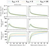 |
Fig. 1. Panels a–c: mass density, sound speed, and radial speed of the solar wind before any injection of a pump wave. The solar-wind response after the injection of a 0.3 mHz pump wave is similarly shown in panels d–f. The solar-wind solutions are presented for the different magnetic flux tube expansion factors: fmax = 3, 5, 10. |
3.2. High-frequency injection: Transient and persisting perturbations
When the frequency of the injected pump wave is increased, persistent large-amplitude perturbations in the solar wind solution are observed. In Fig. 2, we show the deviation of the radial velocity and the outward and inward Elsässer variables from their time-averaged mean values. Specifically, a quantity q (representing either vr, z+ = |z+| or z− = |z−|) is decomposed according to

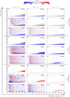 |
Fig. 2. Evolution of perturbations in radial velocity δvr (top three rows), magnitude of the outgoing Elsässer variable δz+ (middle three rows), and magnitude of the incoming (towards the Sun) Elsässer variable δz− (bottom three rows). For each quantity, the results for the flux tube expansions, fmax = 3, 5, and 10, are shown in the left, middle, and right columns, respectively. The frequency of the injected pump wave is indicated in the inset of each panel. |
where q0 is the mean value and δq represents the deviation from the mean, that is, the perturbation. The mean value q0 is calculated by averaging in time from the when the simulation likely reaches a quasi-steady state until the end of the simulation. Thus, we average starting from τ0 = 24 to τ1 = 50 h. The figure presents the progression of time of the perturbations, with the horizontal axis denoting heliocentric distance and the vertical axis the simulation time elapsed (in hours). For each quantity (vr, z+, z−), we display a separate plot for the three flux tube geometries considered, as well as for three selected pump frequencies of 0.5, 1, and 3 mHz. Finally, each of these perturbations are represented in the [ − 400, 400] km s−1 range.
The perturbations induced by the injected monochromatic pump waves require about 10 h to propagate across the simulation domain. This is observed by the initial appearance of a blue region in δz+ and δvr for r > 2 R⊙, signaling a depletion in the quantities. This change is subsequently observed to disappear at t ∼ 10 h. After this initial reconfiguration phase of the corona as a response to the injected waves, perturbations start to appear with a clear dependence both on the pump frequency and flux tube geometry fmax. Perturbations become more persistent with increasing frequency; the frequency at which perturbations become persistent increases with fmax. For instance, δvr, for the lowest investigated pump frequency 0.5 mHz in Fig. 2 (panels a, j, s), exhibits perturbations only in the case of fmax = 3 from 10−20 h. These perturbations for fmax = 3 are advected outwards and cease to be excited, after which point the solar wind attains a steady state. However, these transient perturbations do not arise for fmax = 5, 10. The same behaviour is also detected for δz± at 0.5 mHz. In contrast, for the pump frequency 1 mHz we observe perturbations that persist for the entire duration of the simulation once excited for fmax = 3, while only transient perturbations exist for fmax = 5, similar to the case of 0.5 mHz with fmax = 3 discussed above. Subsequently, with an additional increase in the frequency of the pump wave to 3 mHz, we observe that transient perturbations are generated for fmax = 10, but persist for both fmax = 3 and 5.
The response of the solar wind for a given flux tube expansion factor as it transitions from transient to persistent perturbations can be better understood through Fig. 3. Here, the locations where the radial velocity equals the local Alfvén speed (vr = vA) are plotted in time for the various flux tube geometries. The absolute locations of the crossings are denoted by partially transparent markings, while the arithmetic mean of the locations at a given time are plotted using opaque markings. In Fig. 2, we observe the solar wind exhibiting no large-amplitude perturbations for a 0.5 mHz pump wave and when fmax ≥ 5. Correspondingly, the Alfvén point remains constant after 10 h as seen in Fig. 3 (panel a), except where we have transient perturbations. Thus, in the absence of large-amplitude solar wind perturbations the injection of a pump wave causes the Alfvén point to occur at a lower heliocentric distance, with this decrease being more prominent for a lower fmax. This greater acceleration of the solar wind for a lower flux-tube parameter is similarly observed in Fig. 1. Upon injecting a 0.5 mHz pump wave, the Alfvén point moves from ∼17.5 R⊙ to ∼14.5 R⊙ for fmax = 3, and from ∼6 R⊙ to ∼5 R⊙ for fmax = 10 (Fig. 3). A similar behaviour is also observed for the case of fmax = 10 at 1 mHz. In the case of the short-lived transient perturbations observed from 10−20 h for the cases of fmax = 3 at 0.5 mHz, fmax = 5 at 1 mHz, and fmax = 10 at 3 mHz, we see a sharp deviation in the Alfvén point from the initial steady-state wind. The presence of large-amplitude sustained perturbations in the solar wind causes the Alfvén point to oscillate around the unperturbed locations. For instance, in the case of fmax = 3 at 1 mHz, the Alfvén point oscillates approximately around the same location as in the case of fmax = 3 at 0.5 mHz. Further comparing the evolution of the Alfvén points for fmax = 3 and fmax = 5 at 0.5 mHz with the highest 3 mHz frequency, we observe that the oscillation amplitudes of the Alfvén point decrease with an increase in fmax and pump frequency.
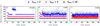 |
Fig. 3. Evolution of Alfvén crossings (vr > vA) with time for the solar-wind conditions in Fig. 2. The opaque markings denote the mean location of these crossings at a given heliocentric distance, while the transparent markings denote the instantaneous locations of the Alfvén crossings. |
The analysis of Alfvén crossings reveals that short-lived transient perturbations for δvr and δz± in Fig. 2 occur as the solar wind advects any reflected waves that are excited beyond the Alfvén point outwards. In Fig. 2, we see that incoming waves (z−) are generated beyond ∼15 R⊙ at t = 8 h for a pump frequency of 0.5 mHz and fmax = 3. The corresponding Alfvén point at this time is ∼14 R⊙ (Fig. 3a). As a consequence, this disturbance is advected outwards by the solar wind, resulting in the short-lived transient perturbations and the jump in the Alfvén point to ∼25 R⊙ between 10 and 20 h. This reasoning similarly applies for fmax = 5 at 1 mHz, and fmax = 10 at 3 mHz.
3.3. Reflected Alfvén waves in the solar wind
In Sect. 3.2, we observed the response of the solar wind upon the injection of a pump wave and the generation of corresponding perturbations leading to varying Alfvén points. Here, we investigate the generation mechanism of the inward propagating (z−) Alfvén wave that is formed as a response to injecting the outward pump wave at certain frequencies. In Fig. 2, we observed the presence of corresponding perturbations in z−, which correlated with persisting perturbations in z+ and vr. As discussed in Sect. 1, Alfvén waves can be reflected due to both the inhomogeneity of the medium as well as the PDI.
In order to quantify the presence of Alfvén waves, we consider the time-averaged component of the Elsässer variables (i.e.  ). The presence of increased Alfvén wave reflections creates suitable conditions for turbulent heating and slow mode generation by modulating the magnetic field, which can lead to fast shocks (Goldreich & Sridhar 1995; Uchida & Kaburaki 1974; Wentzel 1974; Cranmer & Woolsey 2015; Suzuki 2004). These processes in turn contribute to the further increase in density perturbations. As a consequence, it is possible to generate density perturbations in the solar wind, even in the absence of the PDI. To capture the presence of a compressive wave mode we define the time-averaged fractional density fluctuation n as (Shoda et al. 2018b)
where ⟨x⟩ denotes the time-averaged value of x computed as  . Here, we set τ0 = 24 h and τ1 = 50 h. We note that this averaging procedure was performed differently from that used in Eq. (15) as the averaging is here computed dynamically during the simulation run-time using each time-step as an input date. Through defining n as such, we are able to capture the perturbations around the averaged density ⟨ρ⟩. According to Cranmer & Van Ballegooijen (2012), the fractional density fluctuations without PDI and only with reflections is given by δρrms/ρ ⪅ 0.1. Thus, we take the threshold for the large-scale density perturbations arising due to PDI to be of the order of n > 0.1. Subsequently, the presence of any non-zero
  in the absence of large-scale density perturbations indicates Alfvén wave reflections due to medium inhomogeneity.
In Fig. 4, we show the time-averaged outgoing and incoming Elsässer variable magnitudes and the fractional density fluctuation n for all the considered values of fmax and pump frequency. At low frequencies of f = 0.3 mHz, there is minimal development (<50 km s−1) of the incoming  for all the flux tubes. As the frequency of the pump wave increases, the development of
  is clearly observed (panels b, e, and h). However, the threshold frequency at which
  reaches larger amplitudes varies with fmax. For instance, it is ≈0.66 mHz for fmax = 3 and ≈4 mHz for fmax = 10. In addition, for a given fmax value, we observe significant density perturbations for the frequency ranges that exhibit larger peak values for
  . These corresponding features in
  and n therefore indicate the development of the PDI. For instance, the instability is excited after ∼25 R⊙ for fmax = 3 at 0.66 mHz and after ∼13 R⊙ for fmax = 10 at 4 mHz.
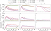 |
Fig. 4. Time-averaged outgoing and incoming Elsässer variables ( |

The mechanism through which reflected Alfvén waves are generated, and particularly the results presented in Figs. 2 and 3, may be identified with PDI. As the quantities shown in Fig. 4 are averaged from 24 h to 50 h, they do not show the transient perturbations that occur in the simulation before this time. However, a similar analysis indicates that short-lived, large-amplitude density perturbations are associated with these phenomena, showing that the transient perturbations are caused by the excitation of the PDI and with the resulting waves advected outwards by the solar wind, since the location at which the instability is triggered is beyond the Alfvén point. In contrast, the presence of persistent perturbations in Fig. 2 are generated by the PDI occurring below the Alfvén point, thereby allowing the waves to remain in the subsonic solar wind. For instance, for the case of fmax = 5 at 3 mHz, we observe sustained perturbations in Fig. 2, with the corresponding Alfvén point oscillating around ∼7 R⊙ (Fig. 3c) and the PDI being excited after ∼3 R⊙.
4. Discussion
4.1. Onset of the PDI
In order to quantify the threshold for the onset of the PDI for the solar wind solutions with different flux tube geometries, we calculate the maximum of the fractional density perturbations nmax and the maximum of the cross-helicity (σc)max. Here, the cross-helicity σc is defined as
Similarly to the definition of n (Eq. (16)), ⟨E±⟩ denotes the time-averaged value of the energy density of the Alfvén waves  averaged over one day for all heliocentric distances in the quasi-steady solution. In a situation with no incoming z− waves, a value of σc = −1 would be obtained. Any departure from this value indicates the presence of a reflected Alfvén wave in the simulation. By comparing the values nmax and (σc)max for the range of pump frequencies and flux tube areas considered, we can investigate the dependence of the threshold for the excitation of the PDI on fmax (Fig. 5). These parameters are indicators of the PDI as this instability generates large-amplitude density fluctuations, which increase n, and reflected Alfvén waves, which increase σc.
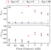 |
Fig. 5. Maximum fractional density perturbations (nmax) and cross-helicity ((σc)max) for the different pump-wave injection frequencies and flux tube geometries. |
In Fig. 5, we observe the dependency of the onset of the PDI on the flux tube geometry. Previous works (Ferraro & Plumpton 1958; An et al. 1990; Velli 1993; Cranmer & Van Ballegooijen 2005; Hollweg & Isenberg 2007) have noted that the reflection of Alfvén waves due to the medium itself is more efficient at lower frequencies. This behaviour is also consistent with the behaviour observed in Fig. 5, where the presence of incoming (z−) waves for 0.3 and 0.5 mHz is indicated by the non-zero values of (σc)max, while simultaneously no large-scale density perturbations are present for all the fmax values. For smaller frequencies of the pump wave, (σc)max is larger, and it progressively decreases until a pump frequency of approximately 0.66 mHz is reached. Thus, we observe that increasing the pump frequency causes a reduction in the generation of reflected Alfvén waves, with the trend continuing monotonically up to a threshold frequency, with the threshold depending on the flux-tube geometry. For instance, a clear jump in nmax and (σc)max is observed to occur for fmax = 3 at 0.66 mHz. This breakdown from the monotonic trend for fmax = 5, 10 is observed at 2 mHz and 4 mHz, respectively. Thus, Fig. 5 indicates the thresholds for the onset of the PDI as the point at which the monotonically decreasing trend of (σc)max breaks down with an accompanying increase in nmax.
This suppression of PDI by the flux-tube expansion factor (fmax) can be explained by considering the plasma beta (Fig. 6). Here, the plasma beta (β) is time-averaged, as defined in Eq. (15) and plotted for pump frequencies 0.3, 1, and 3 mHz. The plasma beta is defined as β = P/(B2/2μ0), where P is the total thermal pressure and B is the magnitude of the total magnetic field. In the absence of PDI, we observe the β ≪ 1 conditions as the solar wind expands (Fig. 6a). The subsequent large-amplitude fluctuations generated by the PDI instability increase the plasma beta as seen for fmax = 3 in Fig. 6b and fmax = 3, 5, 10 in Fig. 6c. Upon comparing Figs. 6a and c, we see that plasma beta increases from < 0.1 to 2 for fmax = 10, but only from ≪0.1 to ≈0.2 for fmax = 3. Thus, the plasma beta is small when fmax is lower, and the relative increase in β is smaller for a lower fmax when the PDI is excited. Previous analytical studies (Galeev & Oraevskii 1963; Sagdeev & Galeev 1969) have shown the inverse dependence of the PDI growth rate on plasma beta (γPDI ∝ β−1/4) in the limit β ≪ 1. Considering the decrease in β as the solar wind expands more slowly (smaller fmax), the onset of PDI is suppressed as the magnetic flux tube expansion factor increases. This variation in the PDI growth rate with fmax is shown by Tenerani & Velli (2013).
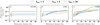 |
Fig. 6. Time-averaged plasma beta (β0) for (a) 0.3 mHz, (b) 1 mHz, and (c) 3 mHz are presented. |
4.2. Acceleration of the solar wind
Comparing the steady-state solar wind solution before the injection of Alfvén waves with the quasi-steady-state solution obtained upon the injection of low-frequency waves, a clear difference in the resulting solar wind speed is seen in Fig. 1. In particular, the terminal wind speed is found to increase with increasing expansion fmax. The same trend is also observed when injecting low-frequency perturbations (Fig. 1f), although the difference in the terminal speeds is smaller in this case.
The wind speeds corresponding to the different flux-tube expansion factors appear contradictory to observations and empirical modelling in which the wind speed has been found to be inversely correlated with the expansion factor (Wang & Sheeley 1990). This apparent difference is caused by the fact that we do not explicitly account for turbulent heating in our present numerical model. In our study, the solar wind is primarily accelerated due to the wave pressure generated by the injected pump wave and the reflected waves, and compressive heating. For a given frequency and flux tube geometry (fmax value), the pump wave is continually injected at a constant amplitude and frequency. This injected pump wave further excites alternate wave modes as a consequence of the PDI (for sufficiently large frequencies). Additionally, we note that a circularly polarised pump wave results in minimal dissipation of heat through direct steepening of outgoing waves to fast shocks (Suzuki 2004; Hollweg 1982). Thus, the variance in the solar-wind acceleration and heating is dependent on the extent of reflected waves. In Fig. 1, we observe that an injection of a 0.3 mHz pump wave causes the wind speed for fmax = 3 to increase the most due to the presence of higher amount of incoming z− waves (see Figs. 4, and 5). Additionally, we observed that the onset threshold for the PDI occurs at a lower frequency for a smaller fmax parameter (Fig. 5).
In addition to the flux-tube expansion geometry, the solar-wind speed is dependent on the magnetic-field magnitude (B0), as has been noted, or example, by Suzuki (2004). In Fig. 7, we compare the radial speed for the various flux-tube geometries for different field strengths varied according to B0 = 2.5, 5, and 10 G. For the case when a pump wave is not injected, we see that fmax = 10 consistently attains the highest terminal speed. Upon the injection of a 0.5 mHz pump wave, we observe the presence of significant perturbations in the radial speed for fmax = 3 at B0 = 2.5 G and fmax = 3, 5 at B0 = 5 G. Similarly to the development of perturbations in Fig. 2, these perturbations of the radial speed correspond to the generation of reflected waves and density perturbations, indicating the development of the PDI for the two cases outlined above. Thus, we observe the presence of greater amounts of reflected waves for a lower B0 as seen in the magnetic field strength (Fig. 7) at which we start observing perturbations in vr for a given fmax parameter. It is to be noted that the case of fmax = 5 at 2.5 G is similar to the short-lived transient perturbations observed in Fig. 2, where the instability occurs after the Alfvén point. Additionally, the injection of the 0.5 mHz pump wave decreases the relative differences in the speeds for different fmax parameters, even in the case when the PDI is not excited (0.5 mHz pump wave at fmax = 10). As stated previously, this variation in speeds is a consequence of the extent of reflected waves generated in our simulation. Subsequently, additional momentum is supplied to the solar wind through the development of alternate wave modes through the development of reflected z− waves, and compressive wave modes. Therefore, for a 0.5 mHz injection the relative scaling of radial speeds for different flux-tube geometries remains the same for B0 = 10 G, while for B0 = 2.5, 5 G the greatest vr is observed for fmax = 3, 5. Finally, in the case with a 3 mHz pump wave that causes the PDI to be excited for all the considered flux tube expansions, we see that the relative difference between the radial speeds for a given field strength B0 shrinks further. Therefore, if we explicitly included a model for turbulent heating in our model the radial speed for fmax = 3 would be expected to be the largest, as in this case we observe the presence of a greater extent of reflected waves as seen by the relative increase in vr from the case without injection of waves. Consequently, the injection of pump waves in a broadband spectrum of frequencies would result in a greater presence of reflected waves for a lower fmax and B0 contributing to a higher acceleration of the solar wind.
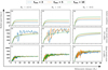 |
Fig. 7. Response of the solar wind for different background magnetic fields (B0 = 2.5, 5, 10 G) and pump-wave injection frequencies (0.5, 3 mHz) are shown. |
5. Conclusion
In this study, we investigated the response of the solar wind upon the injection of a monochromatic pump Alfvén wave. The study is performed considering different magnetic flux-tube expansion geometries (parametrised by fmax) using a single-fluid MHD simulation, which models the non-linear dynamics caused by the pump wave introduced using time-dependent boundary conditions. The model accounts for compressive heating for the range of pump frequencies used in this paper. Thus, given an injection frequency, the model continually injects wave pressure at the low coronal boundary and transfers momentum to the solar wind. This injected Alfvén wave propagates in the solar wind, giving rise to reflected Alfvén waves and compressive wave modes due to the PDI and the inhomogeneity of the medium. Upon injecting the pump wave in quiet solar-wind conditions (Fig. 1), we observed the development of both short-lived and persistent perturbations in our solar-wind solution. An investigation of the reflected Alfvén waves and large-scale density perturbations in Sects. 3.2 and 3.3 indicate the development of the PDI. The solar-wind response and the resulting perturbations (Sect. 3.2) were then explained by the relative positions of the Alfvén point (Fig. 3) and the PDI location, which results in the solar wind advecting the disturbances that occur in the super-Alfvénic region outwards.
Previous works have investigated the dependence of the onset of the PDI on the pump frequency for a single fmax (Shoda et al. 2018a; Réville et al. 2018) and commented on the suppression of the PDI at low frequencies due to efficient reflections of these wave modes. In our study, we found a similar tendency that can be seen in the break of the monotonic trend of (σc)max with the pump frequency in Sect. 4.1. Furthermore, our study finds a strong relationship between the flux-tube expansion and the resulting Alfvén reflections and solar-wind acceleration. In Sect. 4.1, we discussed the PDI threshold for different fmax values which is consistent with the suppression of the PDI by the magnetic flux tube geometry (Tenerani & Velli 2013). Additionally, in Sect. 4.2 we present results that indicate the suppression of the PDI by the increase in magnitude of the background magnetic field (Fig. 7, panels b, e, and h). However, our results displayed an inconsistency with observational results comparing terminal wind speeds for different flux tube expansion factors (Wang & Sheeley 1990). This anomaly is discussed in Sect. 4.2, and the difference was noted to be a consequence of not including an explicit model for turbulent heating in our model. This investigation indicates the importance of considering turbulent heating in order to achieve realistic solar-wind speed profiles, as cited in other works (Suzuki & Inutsuka 2005; Shoda et al. 2018b).
Based on our results, the 1/f scaling of the terminal speed of the solar wind is intimately linked to the turbulent heating, which itself depends intricately on the flux-tube expansion and magnetic field strength. Understanding the coupling of these is a key step in advancing our understanding of the importance of turbulent heating and other processes in accelerating the solar wind.
In the process of performing our study, we experimented with alternate values of the pump-wave amplitude (Eq. (14)) and the parametrisation of the magnetic flux-tube expansion via R1 and σ1 (Eq. (3)). We found that the pump-wave amplitude also inhibits PDI development, with the instability requiring the presence of large amplitude Alfvén waves as considered in our study. Furthermore, the parametrisation in Eq. (3) affects the location at which PDI is excited. The parameters R1 and σ1 in Eq. (3) represent the location and width of the region experiencing the most variation in the flux tube. Thus, alternate choices of these parameters resulted in variance in the location at which the instability is excited without affecting the qualitative behaviour of the solar wind at the given pump frequency and fmax value.
The structure of the solar magnetic flux exhibits a varying expansion factor (fmax) dependent on the heliocentric distance (Griton et al. 2021). In comparison, simulation studies that seek to understand the dynamics of Alfvén wave propagation in the corona employ a fixed fmax derived from a PFSS approximation of the background field. Additionally, previous studies (Pinto et al. 2016) have noted the non-linear dependence of terminal wind speeds on the magnetic flux-tube geometry. Considering the suppression of PDI by the flux-tube geometry and background field studied in this paper, the solar-wind response to Alfvénic fluctuations originating in the photosphere is thus highly sensitive to the approximated magnetic-field geometry. Therefore, through this study we have sought to develop a greater understanding of the validity and formulation of reflection-driven Alfvénic turbulent heating in global simulations of the solar wind and corona. These investigations of the dynamics of Alfvén-wave propagation in the corona are relevant to understanding the near-sun observations of recent spacecraft missions, such as results (Shoda et al. 2021) suggesting an Alfvén origin for magnetic switchbacks in PSP data.
Acknowledgments
The work has been supported by the Finnish Centre of Excellence in Research on Sustainable Space (FORESAIL). This is a project under the Academy of Finland.
References
- Alazraki, G., & Couturier, P. 1971, A&A, 13, 380 [NASA ADS] [Google Scholar]
- An, C.-H., Suess, S., Moore, R., & Musielak, Z. 1990, ApJ, 350, 309 [NASA ADS] [CrossRef] [Google Scholar]
- Banerjee, D., Pérez-Suárez, D., & Doyle, J. 2009, A&A, 501, L15 [NASA ADS] [CrossRef] [EDP Sciences] [Google Scholar]
- Belcher, J., & Davis, L., Jr. 1971, J. Geophys. Res., 76, 3534 [NASA ADS] [CrossRef] [Google Scholar]
- Bowen, T. A., Badman, S., Hellinger, P., & Bale, S. D. 2018, ApJ, 854, L33 [NASA ADS] [CrossRef] [Google Scholar]
- Bruno, R., & Carbone, V. 2013, Liv. Rev. Sol. Phys., 10, 1 [Google Scholar]
- Chandran, B. D. 2010, ApJ, 720, 548 [NASA ADS] [CrossRef] [Google Scholar]
- Chandran, B. D. 2018, J. Plasma Phys., 84, 905840615 [CrossRef] [Google Scholar]
- Coleman, P. J., Jr. 1968, ApJ, 153, 371 [NASA ADS] [CrossRef] [Google Scholar]
- Cranmer, S., & Van Ballegooijen, A. 2005, ApJS, 156, 265 [NASA ADS] [CrossRef] [Google Scholar]
- Cranmer, S. R., & Van Ballegooijen, A. A. 2012, ApJ, 754, 92 [NASA ADS] [CrossRef] [Google Scholar]
- Cranmer, S. R., & Woolsey, L. N. 2015, ApJ, 812, 71 [CrossRef] [Google Scholar]
- D’Amicis, R., & Bruno, R. 2015, ApJ, 805, 84 [Google Scholar]
- De Groof, A., & Goossens, M. 2002, A&A, 386, 691 [NASA ADS] [CrossRef] [EDP Sciences] [Google Scholar]
- Del Zanna, L., Matteini, L., Landi, S., Verdini, A., & Velli, M. 2015, J. Plasma Phys., 81, 325810102 [NASA ADS] [CrossRef] [Google Scholar]
- Derby, N. F., Jr. 1978, ApJ, 224, 1013 [NASA ADS] [CrossRef] [Google Scholar]
- Dewar, R. 1970, Phys. Fluids, 13, 2710 [NASA ADS] [CrossRef] [Google Scholar]
- Dorfman, S., & Carter, T. 2016, Phys. Rev. Lett., 116, 195002 [CrossRef] [Google Scholar]
- Farahani, S. V., Nakariakov, V., Van Doorsselaere, T., & Verwichte, E. 2011, A&A, 526, A80 [NASA ADS] [CrossRef] [EDP Sciences] [Google Scholar]
- Farahani, S. V., Nakariakov, V., Verwichte, E., & Van Doorsselaere, T. 2012, A&A, 544, A127 [NASA ADS] [CrossRef] [EDP Sciences] [Google Scholar]
- Ferraro, C. A., & Plumpton, C. 1958, ApJ, 127, 459 [Google Scholar]
- Fu, X., Li, H., Guo, F., Li, X., & Roytershteyn, V. 2018, ApJ, 855, 139 [NASA ADS] [CrossRef] [Google Scholar]
- Galeev, A., & Oraevskii, V. 1963, Sov. Phys. Dokl., 7, 988 [NASA ADS] [Google Scholar]
- Gary, G. A. 2001, Sol. Phys., 203, 71 [Google Scholar]
- Goldreich, P., & Sridhar, S. 1995, ApJ, 438, 763 [Google Scholar]
- Goldstein, M. L. 1978, ApJ, 219, 700 [NASA ADS] [CrossRef] [Google Scholar]
- Gombosi, T. I., van der Holst, B., Manchester, W. B., & Sokolov, I. V. 2018, Liv. Rev. Sol. Phys., 15, 1 [NASA ADS] [CrossRef] [Google Scholar]
- Goossens, M., Andries, J., Soler, R., et al. 2012, ApJ, 753, 111 [Google Scholar]
- Griton, L., Rouillard, A. P., Poirier, N., et al. 2021, ApJ, 910, 63 [CrossRef] [Google Scholar]
- Hahn, M., & Savin, D. W. 2013, ApJ, 776, 78 [NASA ADS] [CrossRef] [Google Scholar]
- Hartle, R., & Sturrock, P. 1968, ApJ, 151, 1155 [NASA ADS] [CrossRef] [Google Scholar]
- Heyvaerts, J., & Priest, E. R. 1983, A&A, 117, 220 [NASA ADS] [Google Scholar]
- Hollweg, J. V. 1974, J. Geophys. Res., 79, 3845 [NASA ADS] [CrossRef] [Google Scholar]
- Hollweg, J. V. 1982, ApJ, 254, 806 [NASA ADS] [CrossRef] [Google Scholar]
- Hollweg, J. V., & Isenberg, P. 2007, J. Geophys. Res.: Space Phys., 112, 8102 [Google Scholar]
- Hollweg, J. V., Bird, M., Volland, H., et al. 1982, J. Geophys. Res.: Space Phys., 87, 1 [NASA ADS] [CrossRef] [Google Scholar]
- Hollweg, J. V., Cranmer, S. R., & Chandran, B. D. 2010, ApJ, 722, 1495 [NASA ADS] [CrossRef] [Google Scholar]
- Holzer, T. E., & Leer, E. 1980, J. Geophys. Res.: Space Phys., 85, 4665 [CrossRef] [Google Scholar]
- Hoshino, M., & Goldstein, M. 1989, Phys. Fluids B: Plasma Phys., 1, 1405 [NASA ADS] [CrossRef] [Google Scholar]
- Iwai, K., Shibasaki, K., Nozawa, S., et al. 2014, Earth Planets Space, 66, 1 [CrossRef] [Google Scholar]
- Kolmogorov, A. N. 1991, Proc. R. Soc. London Ser. A: Math. Phys. Sci., 434, 9 [NASA ADS] [Google Scholar]
- Kopp, R. A., & Holzer, T. E. 1976, Sol. Phys., 49, 43 [NASA ADS] [CrossRef] [Google Scholar]
- Magyar, N., Van Doorsselaere, T., & Goossens, M. 2017, Sci. Rep., 7, 1 [CrossRef] [Google Scholar]
- Matsumoto, T., & Suzuki, T. K. 2014, MNRAS, 440, 971 [CrossRef] [Google Scholar]
- Mikić, Z., Downs, C., Linker, J. A., et al. 2018, Nat. Astron., 2, 913 [Google Scholar]
- Parker, E. N. 1958, ApJ, 128, 664 [Google Scholar]
- Parker, E. 1960, ApJ, 132, 821 [NASA ADS] [CrossRef] [Google Scholar]
- Pinto, R. F., & Rouillard, A. P. 2017, ApJ, 838, 89 [NASA ADS] [CrossRef] [Google Scholar]
- Pinto, R., Brun, A., & Rouillard, A. 2016, A&A, 592, A65 [NASA ADS] [CrossRef] [EDP Sciences] [Google Scholar]
- Pomoell, J., & Vainio, R. 2012, ApJ, 745, 151 [NASA ADS] [CrossRef] [Google Scholar]
- Pomoell, J., Aran, A., Jacobs, C., et al. 2015, J. Space Weather Space Clim., 5, A12 [NASA ADS] [CrossRef] [EDP Sciences] [Google Scholar]
- Réville, V., Tenerani, A., & Velli, M. 2018, ApJ, 866, 38 [CrossRef] [Google Scholar]
- Sagdeev, R. Z., & Galeev, A. A. 1969, Nonlinear Plasma Theory (New York: Benjamin) [Google Scholar]
- Shoda, M., & Yokoyama, T. 2016, ApJ, 820, 123 [NASA ADS] [CrossRef] [Google Scholar]
- Shoda, M., & Yokoyama, T. 2018, ApJ, 854, 9 [CrossRef] [Google Scholar]
- Shoda, M., Yokoyama, T., & Suzuki, T. K. 2018a, ApJ, 860, 17 [NASA ADS] [CrossRef] [Google Scholar]
- Shoda, M., Yokoyama, T., & Suzuki, T. K. 2018b, ApJ, 853, 190 [Google Scholar]
- Shoda, M., Suzuki, T. K., Asgari-Targhi, M., & Yokoyama, T. 2019, ApJ, 880, L2 [Google Scholar]
- Shoda, M., Chandran, B. D., & Cranmer, S. R. 2021, ApJ, 915, 52 [CrossRef] [Google Scholar]
- Suzuki, T. K. 2004, MNRAS, 349, 1227 [NASA ADS] [CrossRef] [Google Scholar]
- Suzuki, T. K. 2006, ApJ, 640, L75 [NASA ADS] [CrossRef] [Google Scholar]
- Suzuki, T. K., & Inutsuka, S.-I. 2005, ApJ, 632, L49 [NASA ADS] [CrossRef] [Google Scholar]
- Suzuki, T. K., & Inutsuka, S.-I. 2006, J. Geophys. Res.: Space Phys., 111, 6101 [NASA ADS] [CrossRef] [Google Scholar]
- Tenerani, A., & Velli, M. 2013, J. Geophys. Res.: Space Phys., 118, 7507 [NASA ADS] [CrossRef] [Google Scholar]
- Uchida, Y., & Kaburaki, O. 1974, Sol. Phys., 35, 451 [NASA ADS] [CrossRef] [Google Scholar]
- van der Holst, B., Sokolov, I. V., Meng, X., et al. 2014, ApJ, 782, 81 [Google Scholar]
- Velli, M. 1993, A&A, 270, 304 [NASA ADS] [Google Scholar]
- Verdini, A., & Velli, M. 2007, ApJ, 662, 669 [Google Scholar]
- Wang, Y.-M., & Sheeley, N., Jr. 1990, ApJ, 355, 726 [NASA ADS] [CrossRef] [Google Scholar]
- Wentzel, D. G. 1974, Sol. Phys., 39, 129 [NASA ADS] [CrossRef] [Google Scholar]
- Withbroe, G. L. 1988, ApJ, 325, 442 [NASA ADS] [CrossRef] [Google Scholar]
All Figures
|
Fig. 1. Panels a–c: mass density, sound speed, and radial speed of the solar wind before any injection of a pump wave. The solar-wind response after the injection of a 0.3 mHz pump wave is similarly shown in panels d–f. The solar-wind solutions are presented for the different magnetic flux tube expansion factors: fmax = 3, 5, 10. |
| In the text | |
|
Fig. 2. Evolution of perturbations in radial velocity δvr (top three rows), magnitude of the outgoing Elsässer variable δz+ (middle three rows), and magnitude of the incoming (towards the Sun) Elsässer variable δz− (bottom three rows). For each quantity, the results for the flux tube expansions, fmax = 3, 5, and 10, are shown in the left, middle, and right columns, respectively. The frequency of the injected pump wave is indicated in the inset of each panel. |
| In the text | |
|
Fig. 3. Evolution of Alfvén crossings (vr > vA) with time for the solar-wind conditions in Fig. 2. The opaque markings denote the mean location of these crossings at a given heliocentric distance, while the transparent markings denote the instantaneous locations of the Alfvén crossings. |
| In the text | |
|
Fig. 4. Time-averaged outgoing and incoming Elsässer variables ( |
| In the text | |
|
Fig. 5. Maximum fractional density perturbations (nmax) and cross-helicity ((σc)max) for the different pump-wave injection frequencies and flux tube geometries. |
| In the text | |
|
Fig. 6. Time-averaged plasma beta (β0) for (a) 0.3 mHz, (b) 1 mHz, and (c) 3 mHz are presented. |
| In the text | |
|
Fig. 7. Response of the solar wind for different background magnetic fields (B0 = 2.5, 5, 10 G) and pump-wave injection frequencies (0.5, 3 mHz) are shown. |
| In the text | |
Current usage metrics show cumulative count of Article Views (full-text article views including HTML views, PDF and ePub downloads, according to the available data) and Abstracts Views on Vision4Press platform.
Data correspond to usage on the plateform after 2015. The current usage metrics is available 48-96 hours after online publication and is updated daily on week days.
Initial download of the metrics may take a while.